CIRPÉE
Centre interuniversitaire sur le risque, les politiques économiques et l’emploi
Cahier de recherche/Working Paper 05-21
New Evidence on the Determinants of Absenteeism Using Linked
Employer-Employee Data
Georges Dionne
Benoit Dostie
Juin/June 2005
_______________________
Dionne: Canada Research Chair in Risk Management, HEC Montréal, CREF, and CIRPÉE
Dostie: (Corresponding author) CREF, CIRPÉE and Institute of Applied Economics, HEC Montréal, 3000, chemin de la Côte-Sainte-Catherine, Montréal, H3T 2A7. Phone: 514-340-6453; Fax: 514-340-6469
The authors are grateful to seminar participants at the “Journées du CIRPÉE (Knowlton, Québec)”, SCSE (Manoir Richelieu, Québec), CEA (Hamilton, Ontario), and SOLE (San Francisco) and in particular to Pierre Fortin, Pierre
Abstract:
In this paper, we provide new evidence on the determinants of absenteeism using
the Workplace Employee Survey (WES) 1999-2002 from Statistics Canada. Our
paper extends the typical labour-leisure model used to analyze the decision to skip
work to include firm-level policy variables relevant to the absenteeism decision and
uncertainty about the cost of absenteeism. It also provides a non-linear econometric
model that explicitly takes into account the count nature of absenteeism data and
unobserved heterogeneity at both the individual and firm level. Controlling for very
detailed demographic, job and firm characteristics (including workplace practices), we
find that dissatisfaction with contracted hours is a significant determinant of absence.
Keywords: Absenteeism, Linked Employer-Employee Data, Unobserved
Heterogeneity, Count Data Models
1
Introduction
In this paper, we provide new evidence on the determinants of absenteeism using linked employer-employee data. It has long been recognized that while the decision to skip work is made by the individual, reasons for doing so might also be related to personnel considerations or the organizational structure of the firm (Frankel (1921)). Linked data thus provides a unique opportunity to disentangle conflicting causes of absenteeism.
Despite its rising frequency and associated cost, there are relatively few studies on the determinants of absenteeism. Moreover, it could be argued that most of the existing studies on the determinants of absenteeism suffer from the use of less than adequate data. A first strand of the literature focuses on only one kind of absenteeism, namely absenteeism due (officially) to health reasons. These studies generally use data from a health insurance company or government agency.1 A second strand of the literature uses detailed absenteeism data from one company or a very small sample of firms2. It is not clear that their results are generalizable outside their small samples.3,4,5
Our work is thus more closely related to the second strand of the literature
1For example, Henrekson and Persson (2004) use aggregate data from the National Social Insurance Board of Sweden, Johansson and Palme (2002) use data from the 1991 Swedish Level of Living Survey (SLLS). In the U.S., Vistnes (1997) uses the 1987 National Medical Expenditure Survey.
2Kauermann and Ortlieb (2004) have absenteeism data from one German firm. Barmby (2002) also has data on only one UK manufacturing firm. Delgado and Kiesner (1997) focus on London buses operators. Drago and Wooden (1992) work on a sample of 15 firms from the U.S., Canada and New-Zealand. Barmby, Orme, and Treble (1991) use data on four factories of an unidentified firm. Wilson and Peel (1991) have data on a sample of 52 firms in the engineering and metal industry in the United Kingdom. Dunn and Youngblood (1986) use 1977 data from one utility company.
3A notable exception is Allen (1981) who uses the 1972-73 Quality of Employment Survey. However, this survey does not have any information about the employer and therefore cannot be used to study the link between workplace practices and absenteeism.
4Other papers focusing on absenteeism include Gilleskie (1998) who focuses on the ab-senteeism decision of individuals with acute illnesses, Ehrenberg (1970) who studies the link between absenteeism and the decision of the firm to use overtime, and Allen (1983) who estimates the cost of absenteeism.
5A third strand takes a more macroeconomic approach. For example, Kenyon and Dawkins (1989) use aggregate Australian time-series data.
using employee level data. However, we examine the determinants of absen-teeism using survey data, the Workplace Employee Survey (WES) 1999-2002 from Statistics Canada. The use of WES has numerous advantages for the study of the determinants of absenteeism: (1) the survey is designed to be represen-tative of the whole universe of firm operating in Canada; (2) in each sampled firm, a subset of workers from the firm was sampled so that the survey is also representative of the universe of workers in Canada6; (3) since the survey is linked, we have detailed micro data on each of these workers, including days of absenteeism during the year, demographic and job characteristics, preferences and human capital variables (this is in addition to the usual firm-level charac-teristics); (4) each worker was asked to recall the number of days absent from work in the past year; (5) the linked nature of the data allows us to take into account firm unobserved heterogeneity; (6) and the longitudinal nature of the data allows us to take into account worker unobserved heterogeneity.
We start first by extending the typical labor-leisure model used to analyze the decision to skip work to include firm-level policy variables relevant to the ab-senteeism decision and uncertainty about the cost of abab-senteeism to the worker. We next describe an econometric model that explicitly takes into account the count data nature of absenteeism data and also incorporates unobserved het-erogeneity at both the individual and firm level. Data sources and variable descriptions are presented in Section 4. We describe the results in section 5 and briefly conclude in the final section.
6Abowd and Kramarz (1999) classify WES as a survey in which both the sample of work-places and the sample of workers are cross-sectionally representative of the target population.
2
Theoretical Framework
We use the typical labor-leisure choice model to study the absenteeism decision (see Allen (1981), Allen (1983), Barmby, Orme, and Treble (1991), Delgado and Kiesner (1997) and Dunn and Youngblood (1986))7. We assume that each job offers a work schedule as well as a wage rate. Since search is costly, a worker may accept a job offer even though at the contracted number of work hours (tc)
his marginal rate of substitution between leisure and income does not equal the wage rate (w). When a worker contracts for more than his desired hours given
w, he retains an incentive to consume more leisure. One way of doing so is to
be absent from work. In this theoretical framework, an emphasis will be placed on the explicit random cost of such a decision and on how the firms and jobs characteristics affect this decision. These two aspects will become important in the empirical part of the paper and have not been addressed in the literature.
Absenteeism results in lost output when the absent worker is replaced by someone who is generally less efficient or is not replaced at all. For the em-ployment relation to continue, the firm must be compensated for this loss. In addition to losing earnings he would have received if he had reported, the worker faces a penalty (D) for each scheduled work period missed. In practice, this penalty will be observed in the form of a decreased probability of receiving a promotion or merit wage increase and an increased likelihood of being dismissed. Denoting time absent form work as ta, one can then write
D = D (ta) D0 ≥ 0, D00≥ 0, D (0) = 0
The workers who miss the most days pay the largest penalties. The costs of in-creased amounts of absenteeism to the firm are presumed to be non-decreasing,
7The following discussion is also drawn from Vistnes (1997) and Johansson and Palme (1996). See Hausman (1980) and Blomquist (1983) for the foundations of the basic model.
yielding a constant or graduated penalty structure. Workers with perfect atten-dance records are not penalized at all. Since the worker does not really know this potential cost when he makes his decision, we consider the possibility that
D (ta) can be a random variable. So, we write eD (ta) when this is the case.
Holding work schedule flexibility constant, the work attendance decision can be analyzed within the traditional labor-leisure choice framework. Workers maximize an expected utility function containing consumption (C) and leisure time (L) as its arguments8
EU = EU (C, L; P, F ) . (1)
The expected utility of the worker is also a function of a vector of personal characteristics (P ) and a vector of firm characteristics (F ). Letting R equal the individual non-labor income, the budget constraint of the worker is
R + w (tc− (1 − s
L)ta) − eD (ta) = C (2)
where the price of the consumption good C is normalized to one and sL is a
variable that takes the value of one if a worker has full sick leave benefits9 and less than one otherwise. Workers also face a time constraint of
t − tc− ta− tl= 0 (3)
where t represents the total amount of time in the period under consideration and tlis leisure hours. So we can write ta+ tl= L. Substitution of (2) and (3)
8See Dionne and Eeckhoudt (1987) for such a theoretical framework.
9We use the same hypothesis as Vistnes (1997) of modelling sLas a binary variable due to data limitations. As in Vistnes (1997), detailed information on sick leave provisions, such as the stock of sick leave, carry-over provisions, whether sick leave benefits pay the worker fully or partially, and wheter the sick leave can be applied toward early retirement or used for maternity leave, is not available. Detailed job characteristics in the empirical analysis may serve as proxies for these provisions.
in (1) and differentiation of the latter with respect to taproduces the first-order
condition
EhUL− (w (1 − sL) + eD0(ta))UC
i
= 0 (4)
where Uk > 0 indicates the partial derivative of U with respect to k = L, C.
The variable eD (ta) can be expressed more directly by defining wa as the cost
of being absent. So we can write eD (ta) = wata and, as already mentioned, wa
can be a random variable when the decision on tais made. In this case, the first
order condition (4) becomes
E [UL− (w (1 − sL) + wa) UC] = 0. (5)
A worker will be absent on any given day as long as the extra leisure is more valuable to him than the sum of the wages he would have earned that day and the resulting loss in future earnings. This means that the shadow price of time for absent workers is greater than the contracted wage.
By differentiating the first-order conditions for sL = 0 and applying Cramer’s
Rule, one can show, under the usual conditions of an upward sloping labor supply curve, that
∂ta ∂w < 0, ∂ta ∂R > 0, ∂ta ∂tc > 0, ∂ta ∂Risk < 0, ∂ta E (wa)< 0. (6)
where Risk is a measure of the risk associated to wa and E (wa) its mean. See
Dionne and Eeckhoudt (1987) for a sufficient condition yielding dta/dRisk < 0.
(Details for the derivation of results in (6) are in Appendix).
The effect of a change in the wage rate on time absent from work is am-biguous a priori because income and substitution effects operate in opposite directions. However, under the conditions of an upward sloping labor supply curve, a negative sign is obtained when sL = 0 or is sufficiently small. An
in-crease in non-labor income leads to more demand for all non-inferior goods and services, including time absent from work. If the number of contracted hours changes, the number of absences move in the same direction. Increased penal-ties for absenteeism reduce the number of days missed; as does an increased risk of penalty.
In cases where full sick leave is available, the product of w and ta disappears
from (2) and the first–order equilibrium condition becomes
E [UL− waUC] = 0. (7)
Unless the penalty function is made steeper, an individual will be absent more frequently in plants where sick leave is fully paid to absent workers. It should be noted that the effect of a wage change on the likelihood of absence is unam-biguously positive in this case because there is no longer a substitution effect.
Denoting the scheduling flexibility permitted by one’s employer as f (we expect ∂tA/∂f < 0), the model can be summarized as
tA= tA( w, R, tc, E(wa), Risk, f ).
(−) (+) (+) (−) (−) (−)
(8)
We provide a structural form for these relationships in the next section.
3
Empirical Specification
From the above behavioral model, we can derive a structural econometric model of the absenteeism decision. Extending the model of Hausman (1980) and Blomquist (1983) proposed for labor force participation, we can write the
fol-lowing functional form for the utility function: U¡C, ta+ tl; P, F¢= exp ( − Ã 1 + β ¡ C + P + F¢ b − t + (ta+ tl) !) Ã t −¡ta+ tl¢− b β ! (9) where P = P/β − α/β2, F = F/β − α/β2, b = α/β,
α and β are parameters and absolute risk aversion is assumed equal to one10. From this utility function, one can verify that the first order condition yields
ta = tc− α¡w (1 − sL) + E (wa) + 1/2σ2
¢
− β (R + tcwsL) − γP − ηF (10)
assuming normal distribution for wa, which yields σ2as the measure of risk. In a more compact form, (10) can be rewritten as
ta= tc− αw∗− βR∗− γP − ηF
where w∗ can be interpreted as the relative cost of being absent and R∗ as the
virtual benefit or income related to absence. A positive α parameter and a negative β parameter are expected.
In this simple model, when preferences are not random, days of absenteeism can be represented by a Poisson process (see Hausman, Hall, and Griliches (1984); Gouri´eroux, Monfort, and Trognon (1984)). In fact, since absences are recorded as non-negative integers, modeling such data with a continuous distribution could lead to inconsistent parameter estimates. Let ta
ijt be the
observed number of days of absenteeism for employee i in firm j at time t. The
10See Johansson and Palme (1996), for a similar model where the firms variables are not considered and wais not present in the budget constraint.
basic model is P (taijt | λijt) = e−λijt(λ ijt)t a ijt ta ijt! (11) with
λijt= tcijt− αw∗ijt− βR∗ijt− γPit− ηFjt> 0.
It should be repeated that tc
ijt (contracted hours) are exogenous in the model.
This decision variable is already fixed when the worker (or nature) makes a decision about ta.
It is typical to introduce unobserved heterogeneity in the Poisson model in a multiplicative form through λijt. Unobserved heterogeneity should be present
because many non observable factors in the data set can affect the sensitivity to economic incentives related to work absence decisions. We use the following parameterization for λijt
λijt= exp(δij+ ψj+ θij) (12)
where
δij= tcijt− αw ∗
ijt− βR∗ijt− γPit− ηFjt
The additional parameter ψj captures unobservable factors of the firm
orthog-onal to other observed firm characteristics. We assume firm unobserved hetero-geneity to be normally distributed with mean zero. The variance of ψj (σψ) is
identified by the observation of many workers coming from the same firm. Since we do not observe worker mobility due to the design of the survey, we do not include pure worker unobserved heterogeneity but because of the longitudinal nature of the data, we have repeated observations on the employer-employee relationship which allows us to take into account unobserved job het-erogeneity (θij). We also assume that θij is distributed normally with variance
σθ and is orthogonal to ψj11. Firm unobserved heterogeneity might proxy for
the cost of absence to the firm when observed heterogeneity is not sufficiently informative. For example, the cost of absence to the firm might be pretty low if substitute workers are easily available and are as productive as regular workers (Allen (1983)) and therefore, the econometrician might observe higher absen-teeism than in an otherwise identical firm where such substitute workers are not available. From a statistical point of view, it is necessary to take into account both sources of heterogeneity in order to avoid the problem of spurious regres-sions due to multiple observations on the same worker over time and the same firm characteristics over its employees.
The joint likelihood is obtained by numerically integrating out the hetero-geneity components from the product of the conditional likelihoods of the firms, assuming joint normality of the heterogeneity components. Since a closed form solution to the integral does not exist, the likelihood was computed by approx-imating the normal integral by a weighted sum over “conditional likelihoods”, i.e. likelihoods conditional on certain well-chosen values of the residual.
4
Data
We use data from the Workplace and Employee Survey (WES) 1999-2002 con-ducted by Statistics Canada. The survey is both longitudinal and linked in that it documents the characteristics of the workers and of the workplaces over time. The target population for the “workplace” component of the survey is defined as the collection of all Canadian establishments who paid employees in March of the year of the survey. The survey, however, does not cover the Yukon, the Northwest territories and Nunavut. Establishments operating in fisheries,
agri-11Note that this specification is not subject to the usual objections to the Poisson model since the inclusion of firm and worker unobserved heterogeneity allows for dispersion at both the worker and firm level.
culture and cattle farming are also excluded. For the “employee” component, the target population is the collection of all employees working, or on paid leave, in the workplace target population.
The sample for the workplaces comes from the “Business registry” of Statis-tics Canada which contains information on every business operating in Canada. Employees are then sampled from an employees list provided by the selected workplaces. For every workplace, a maximum of twelve employees are selected, and for establishments with less than four employees, all employees are sampled. In the case of total non-response, respondents are withdrawn entirely from the survey and sampling weights are recalculated in order to preserve representa-tiveness of the sample. WES selects new employees and workplaces in odd years (at every third year for employees and at every fifth year for workplaces). We used the final sampling weights for employees as recommended by Statistics Canada in all our regressions.
We finally exclude establishments with less than ten employees from the sample because survey questions on work practices were not intended for them. Individuals who did no work throughout the year are also included but we control for their limited exposure to the risk of being absent in our regression framework. The rich structure of the data set allows us to control for a variety of factors determining absenteeism decisions. From the worker questionnaire, we are able to extract detailed demographic characteristics including measures of health, human capital, job satisfaction and income from other sources. More-over, we use detailed explanatory variables on the employment contract includ-ing wage, contracted hours and information about workinclud-ing hours flexibility and when these working hours take place.
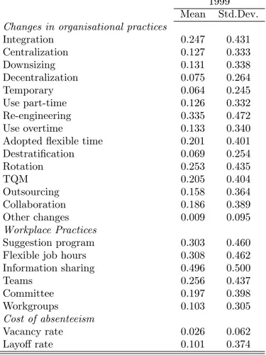
From the firm questionnaire, we are able to construct firm size indicators and build measures of turnover and vacancy rates. Even more important, the
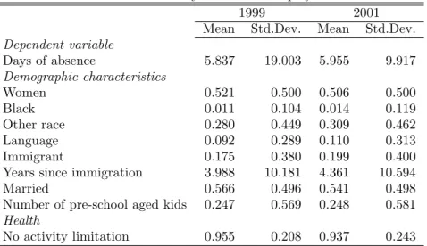
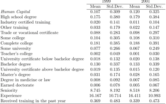
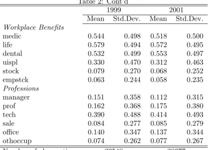
establishment questionnaire includes very detailed information about changes in organizational practices (15 indicators) and current workplace practices (6). We complement those by adding some indicators for the type of nonwage benefits that the firm offers to its workers. Finally, our regressions include industry (13), occupation (6) and time (4) dummies. Summary statistics on all explanatory variables are presented in Table 1 for the dependent variable, Table 2 for the employees and Table 3 for the employer. Note that week absent in Table 1 refers to a five day workweek. Thus zero means the worker was absent strictly less than five days.
5
Results
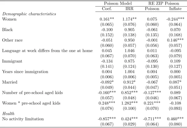
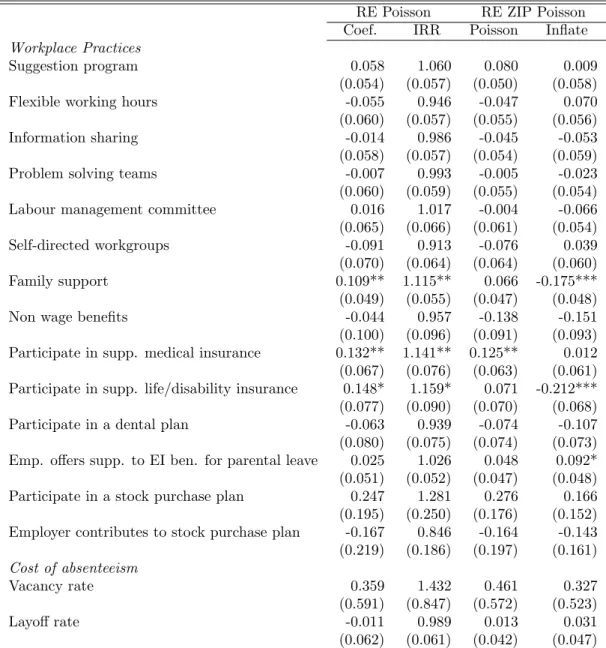
Complete estimation results are presented in the multiple parts of Table 4. The first column presents results from the estimation of the standard Poisson model from equation (12) and column “IRR” shows the corresponding incidence rate ratios. The two next columns show estimation results from a zero-inflated Pois-son (ZIP) model. This other model accounts for the prevalence of zero counts in the absenteeism data. The ZIP Poisson model also takes into account the fact that the determinants of zero counts could be different from the determinants of the number of days of absenteeism, due to job design or matching in the job market for example.
In all models, the dependent variable is the number of days of absence that are reported for the whole year. Note that the survey distinguishes between paid sick leave, unpaid leave and other paid leave12. Using days of absence in this type of survey might be problematic if the distribution of days of absence is not smooth. Moreover, it is possible that the respondent’s ability to recall absences
12Other paid leave does not include vacations, paternity/maternity leave or absence due to strikes or lock-out.
for a full year is not as good as we would like it to be13. For these reasons, in our empirical analysis, we also tested the model using weeks of absenteeism as the dependent variable. Since results did not differ, we show only results for days of absenteeism14.
Note that we were not able to estimate the full specification with parametriza-tion (12) since the firm and employee random effects are not nested. Non-linear models with more than one variance component are very hard to estimate due to their high dimensionality, especially if the random effects are not nested, which is the case with firm and individual heterogeneity. Many methods have been proposed to overcome such numerical difficulties (see Lee and Nelder (1996) and Jiang (1998)) but unfortunately, it turns out that none are robust enough to deal with data sets of the size we use in this analysis. We compared results between two specifications, workplace or worker unobserved heterogeneity and since results did not differ much between the two specifications, we present re-sults including worker heterogeneity only. Finally, in what follows, we focus mainly on coefficients and incidence rate ratios from the Poisson model but discuss results from the ZIP model when they differ.
Demographics and health We find that women are likely more likely to be absent. Women have 1.17 times the absence rate of men and this effect is even stronger if there are kids younger than six years old in the household15. Being married reduces absenteeism but the effect is significant at the 10% level only. Health is also found to be a very important determinant of the absen-teeism decision. Individuals with no activity limitation have less than half the incidence rate of individuals with activity limitations. The impact of health
13Unfortunately, it is not possible to compare the number of absences as reported by the worker to administrative measures.
14The structure of the data also does not allow us to study episodes of absenteeism. 15Vistnes (1997) also finds a significant interaction between being a women and having young kids.
is slightly less important in the ZIP model but also a statistically significant positive determinant of the probability of having no absenteeism which suggests that individuals with activity limitations will also be matched with jobs where absenteeism is permitted
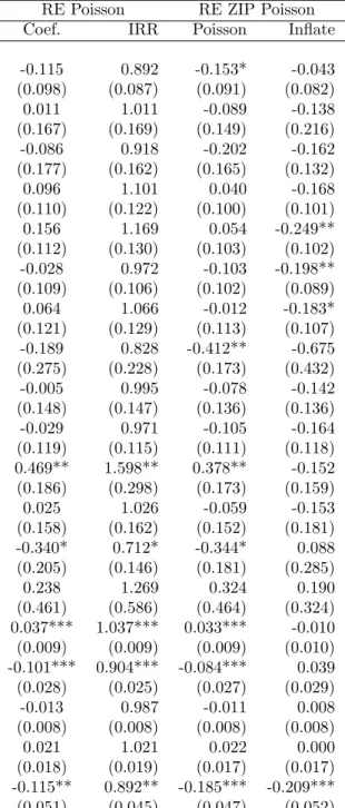
Human capital Even with the detailed data we have on degrees obtained, we find almost no impact of schooling on absenteeism except for the category “University certificate above bachelor degree”. The only two measures of human capital that are related to absenteeism decisions are seniority (positive but at a diminishing rate) and whether the individual received training in the past year (negative).
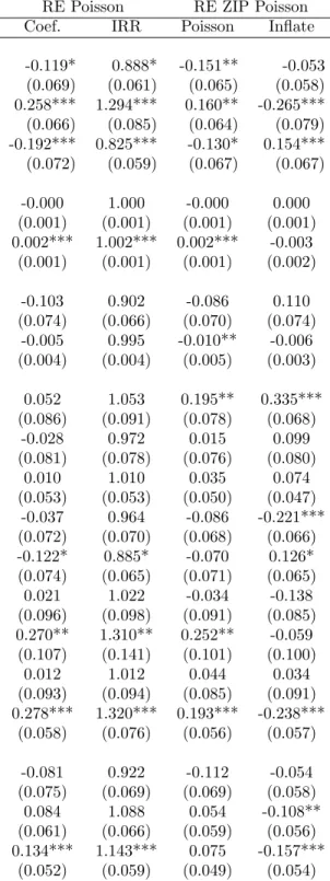
Preference and job satisfaction We find very strong evidence that dis-satisfaction with job contracts is related to absence. Workers who indicated that they would prefer to work more hours for more pay are less often absent and workers who would prefer to work less hours for less pay are more often absent. We think this is the strongest evidence yet that absenteeism decisions act as a mechanism to adjust hours to the worker’s optimal schedule. Job sat-isfaction is also strongly related to absence. Workers who reported being very satisfied or satisfied with their job have 0.83 times the absence rate of dissatisfied individuals.
Income, wage and hours We find that, as predicted by our theoretical model, increasing income from other sources is related to more absence. The coefficient on wages is negative as predicted although the effect is not signifi-cant. We get a negative sign for contracted hours but the effect is very small. This could be due to the fact that a fair share of our sample does not work regular hours every week. Since we do not observe the contract, our measure
of contracted hours is more a measure of the number of usual hours worked on average per week.
Work arrangement and technology use It has been said that new work arrangements lead to more stress and more absenteeism. Using detailed data about the scheduling of the work week, we find that workers who are able to do part of their work at home are less often absent and that workers who work on a reduced workweek are more often absent. Turning to technology, we find that workers using other technologies (such as cash registers, sales terminals, scanners, etc) have a higher incidence rate of absenteeism.
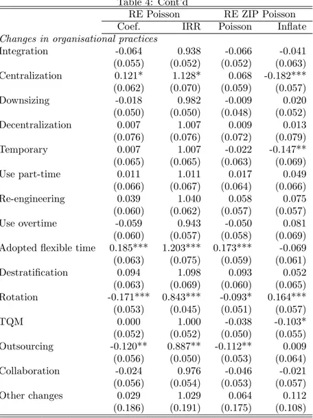
Organizational change Firms would normally be interested in finding what organizational practices succeed in reducing absenteeism when it is costly. We find that centralization and the introduction of flexible working hours in the firm are associated with higher absenteeism, while job rotation (or multi-skilling) and outsourcing are related to lower absenteeism16. It is interesting to contrast the impact of these organizational changes in the ZIP model. For example, the impact of outsourcing shows up only in the Poisson part of the ZIP model while the impact of centralization shows up only in the inflated part. This means that outsourcing is associated with reduced incidence of absenteeism while central-ization is probably associated with reduction in “permitted” absenteeism in the job design.
Workplace practices We find no impact for flexible job design, sugges-tion programs, informasugges-tion sharing, the use of solving teams, labour-management committees and self-directed workgroups on absenteeism17. We do however find
16In separate work, we look at correlations between individual workplace practices in order to verify if some practices were most likely to be used in conjunction with others. Since no correlation is above 0.5, we decide against using “bundles” of practices.
17Drago and Wooden (1992) find that workgroup cohesion is associated with lower levels of absence if job satisfaction is high and Wilson and Peel (1991) find that firms with participation
that workplaces that offer family support have more absences, but this effect works through the inflated part of the Poisson model which suggests it is also due to job design.
Cost of absenteeism We construct two measures of the indirect cost of absenteeism. We make the hypothesis that the worker is less likely to be penalized for his absence (through lower promotion probabilities) if vacancy rates are high and layoff rates are low. Although we find that our coefficients have the expected effects, neither are statistically significant.
Firm size, occupations, industry and time effects We find absen-teeism to be greater in large firms and for all occupations compared to man-agers. Interestingly, we find no interindustry differentials in the incidence of absenteeism but the large majority of industry dummies18 are statistically sig-nificant in the inflated part of the ZIP model which suggests big industry differ-ences in job design. Finally, all year dummies are negative. Since the reference year is 1999, we conclude that increases in absenteeism in that time period were probably due to changes in the workforce composition and job mix.
6
Conclusion
In this paper, we provide a careful examination of the factors associated with the absenteeism decision at the worker level using survey data where the infor-mation on the worker is linked to inforinfor-mation about the workplace, something that has rarely been done. The data we use allow us to control for detailed demographic worker, job and firm characteristics. We find strong evidence that dissatisfaction with contracted hours is related to absence. We find that most
schemes had significantly lower average absenteeism. These findings are not corroborated by our data.
human capital effects work through seniority and training. The predictions of our theoretical model are consistent with our results except for the coefficient on contracted hours which may be due to measurement error. We do not find strong indications that non traditional work arrangement lead to absenteeism. But the possibility of working at home is associated with lower absences. We find that firms that showed increased reliance on external suppliers (outsourc-ing) also saw absenteeism diminish.
Future work should be on devising estimation methods that would take into account the linked nature of the data. Such an estimation framework could be based on Monte Carlo Markov Chain methods to take into account the fact that the firm and worker effects are not nested. Also, it would be interesting to see if the determinants of absenteeism differ depending on the type of absenteeism (paid/unpaid, sick leave/other leave).
References
Abowd, J. M. and F. Kramarz (1999). The analysis of labor markets using matched employer-employee data. In O. Ashenfelter and D. Card (Eds.),
Handbook of Labor Economics, vol 3B, Chapter 40, pp. 2629–2710.
Else-vier Science North Holland.
Allen, S. G. (1981). An empirical model of work attendance. Review of
Eco-nomics and Statistics 63 (1), 77–87.
Allen, S. G. (1983). How much does absenteeism cost. Journal of Human
Resources 18 (3), 379–393.
Barmby, T. (2002). Worker absenteeism: a discrete hazard model with bivari-ate heterogeneity. Labour Economics 9, 469–476.
analysis using microdata. Economic Journal 101 (405), 214–229.
Blomquist, N. S. (1983). The effect of income taxation on the labor supply of married men in sweden. Journal of Public Economics 22 (2), 169–197. Delgado, M. A. and T. J. Kiesner (1997). Count data models with variance of
unknown form: An application to a hedonic model of worker absenteeism.
Review of Economics and Statistics 79 (1), 41–49.
Dionne, G. and L. Eeckhoudt (1987). Proportional risk aversion, taxation and labour supply under uncertainty. Journal of Economics 47 (4), 353–366. Drago, R. and M. Wooden (1992). The determinants of labor absence:
Eco-nomic factors and workgroup norms across countries. Industrial and Labor
Relations Review 45 (4), 764–778.
Dunn, L. and S. A. Youngblood (1986). Absenteeism as a mechanism for approaching an optimal labor market equilibrium: An empirical study.
Review of Economics and Statistics 68 (4), 668–674.
Ehrenberg, R. G. (1970). Absenteeism and the overtime decision. American
Economic Review 60 (3), 352–357.
Frankel, E. (1921). Labor absenteeism. Journal of Political Economy 29 (6), 487–499.
Gilleskie, D. B. (1998). A dynamic stochastic model of medical care use and work absence. Econometrica 66 (1), 1–45.
Gouri´eroux, C., A. Monfort, and A. Trognon (1984). Pseudo maximum like-lihood functions: Applications to poisson models. Econometrica 52 (3), 701–720.
Hausman, J., B. Hall, and Z. Griliches (1984). Econometric models for count data with an application to the patents-r&d relationship.
Hausman, J. A. (1980). The effect of wages, taxes, and fixed costs on women’s labor force participation. Journal of Public Economics 14 (2), 161–194. Henrekson, M. and M. Persson (2004). The effects on sick leave of changes in
the sickness insurance system. Journal of Labor Economics 22, 87–113. Jiang, J. (1998). Consistent estimators in generalized linear mixed models.
Journal of the American Statistical Society 93 (442), 720–729.
Johansson, P. and M. Palme (1996). Do economic incentives affect work ab-sence? empirical evidence using Swedish micro data. Journal of Public
Economics 59, 195–218.
Johansson, P. and M. Palme (2002). Assessing the effect of public policy on worker absenteeism. Journal of Human Resources 37, 381–409.
Kauermann, G. and R. Ortlieb (2004). Temporal pattern in number of staff on sick leave: the effect of downsizing. Journal of the Royal Statistical
Society Series C - Applied Statistics 53, 355–367.
Kenyon, P. and P. Dawkins (1989). A time series analysis of labour absence in australia. Review of Economics and Statistics 71 (2), 232–239.
Lee, Y. and J. Nelder (1996). Hierarchical generalized linear models. Journal
of the Royal Statistical Society B 58 (4), 619–678.
Vistnes, J. P. (1997). Gender differences in days lost from work due to illness.
Industrial and Labor Relations Review 50 (2), 304–323.
Wilson, N. and M. J. Peel (1991). The impact on absenteeism and quits of profit-sharing and other forms of employee participation. Industrial and
A
Comparative Statics of t
aDecision with Respect to Different Parameters The first order condition with respect to ta is equal to:
E [UL− (w (1 − sL) + wa) UC] = 0.
We write H < 0 for the second order condition that is easily verified under risk aversion. We assume that leisure is not an inferior good.
So differentiating with respect to R yields:
dta dR = − 1 HE ¡ ULC− wtUCC ¢ > 0
when L is not an inferior good under certainty. Now differentiating with respect to w yields:
dta dw = 1 HEUC(1 − sL) − 1 HE ¡ ULC− wtUCC ¢ (tc− (1 − s L) ta) where wt≡ w (1 − sL) + wa > 0.
This can be rewritten as
dta dw = − 1 HE £ − (1 − sL) UC+ ¡ ULC− wtUCC ¢ (tc− (1 − s L) ta) ¤
which is negative under normal conditions of positive labor supply curve and when sL= 0 or small. When sL= 1, the effect is positive.
The sign of dta/dtc is given by the sign
dta dtc = − 1 HE £ ULC− wtUCC ¤ w > 0.
The sign of dta/dE (wa) is the same as that of dta/dwa under certainty. dta dE (wa) = − 1 HE £ −UC− ¡ ULC− wtUCC ¢ ta¤< 0
when L is not an inferior good under certainty. Finally, the sign of dta/d (Risk) is that of
dta d (Risk) 1 ta = UCC(1 − t aI) + U Cta ∂I ∂wa < 0 where I ≡ULC− w tU CC UC > 0
if leisure is not an inferior good: 1 − taI is positive when the supply curve of
labor is positive and ∂I/∂wa is non-increasing using an intuitive condition on
the variation of proportional risk aversion along the budget line (see Dionne and Eeckhoudt (1987), for more details).
Table 1: Summary statistics on absenteeism in Canada (1999) Weeks absent Freq. % 0 9,717,342 90.16 1 669,090 6.21 2 185,702 1.72 3 25,927 0.24 4 31,343 0.29 5 7,437 0.07 6 22,676 0.21 7 14,159 0.13 8 15,538 0.14 9 10,675 0.10 10 3,986 0.04 (...) (...) Total 10,777,543 100.00
Table 2: Summary statistics - Employees
1999 2001
Mean Std.Dev. Mean Std.Dev.
Dependent variable Days of absence 5.837 19.003 5.955 9.917 Demographic characteristics Women 0.521 0.500 0.506 0.500 Black 0.011 0.104 0.014 0.119 Other race 0.280 0.449 0.309 0.462 Language 0.092 0.289 0.110 0.313 Immigrant 0.175 0.380 0.199 0.400 Years since immigration 3.988 10.181 4.361 10.594
Married 0.566 0.496 0.541 0.498
Number of pre-school aged kids 0.247 0.569 0.248 0.581
Health
Table 2: Cont’d
1999 2001
Mean Std.Dev. Mean Std.Dev.
Human Capital 0.107 0.309 0.120 0.325
High school degree 0.175 0.380 0.179 0.384 Industry certified training 0.020 0.141 0.011 0.104 Other training 0.033 0.179 0.022 0.147 Trade or vocational certificate 0.088 0.283 0.098 0.297
Some college 0.104 0.305 0.108 0.310
Complete college 0.181 0.385 0.188 0.391 Some university 0.077 0.266 0.067 0.249 Teacher’s college 0.002 0.049 0.001 0.030 University certificate below bachelor degree 0.018 0.132 0.020 0.138 Bachelor degree 0.130 0.337 0.133 0.339 University certificate above bachelor degree 0.019 0.135 0.015 0.120 Master’s degree 0.031 0.174 0.028 0.165 Degree in medicine or law 0.008 0.092 0.007 0.085 Earned doctorate 0.006 0.078 0.005 0.067
Seniority 8.745 8.192 8.518 8.206
Experience 16.167 10.714 16.411 10.993 Received training in the past year 0.369 0.483 0.339 0.473
T able 2: Con t’d 1999 2001 Mean Std.Dev. Mean Std.Dev. Pr efer enc es and Job Satisfaction W ould prefer to w ork more hours for more pa y 0.191 0.393 0.217 0.412 W ould prefer to w ork less hours for less pa y 0.097 0.296 0.069 0.253 Satisfied with job 0.893 0.309 0.898 0.302 Inc ome T otal family income 65901.390 54371.310 65353.690 43994.350 Income from other sources 2325.539 11835.740 2609.757 12282.100 Wage Contr act Natural logarithm of hourly w age 2.778 0.521 2.820 0.530 Con tracted hours 36.623 9.837 36.237 9.711 Work arr angement W orks regular hours 0.141 0.348 0.137 0.344 Usual w orkw eek includes Saturda y and Sunda y 0.185 0.388 0.225 0.417 W ork flexible hours 0.396 0.489 0.352 0.477 Do es not w ork from Monda y to F rida y b et w een 6am and 6pm 0.647 0.478 0.584 0.493 Some w ork done at home 0.267 0.443 0.231 0.422 W ork some rotating shift 0.048 0.214 0.070 0.256 W ork on a reduced w orkw eek 0.049 0.215 0.079 0.269 W ork on compressed w ork w eek sc hedule 0.031 0.173 0.055 0.228 Co vered b y a collectiv e bargaining agreemen t 0.279 0.449 0.280 0.449 W ork part time 0.051 0.220 0.053 0.224 T echnolo gy Use computer 0.608 0.488 0.601 0.490 Use computer assisted design 0.120 0.325 0.133 0.340 Use other tec hnology 0.269 0.443 0.228 0.420 Workplac e Pr actic es F amilySupp ort 0.313 0.464 0.338 0.473 Non w age 0.678 0.467 0.712 0.453
Table 2: Cont’d
1999 2001
Mean Std.Dev. Mean Std.Dev.
Workplace Benefits medic 0.544 0.498 0.518 0.500 life 0.579 0.494 0.572 0.495 dental 0.532 0.499 0.553 0.497 uispl 0.330 0.470 0.312 0.463 stock 0.079 0.270 0.068 0.252 empstck 0.063 0.244 0.058 0.235 Professions manager 0.151 0.358 0.112 0.315 prof 0.162 0.368 0.175 0.380 tech 0.390 0.488 0.414 0.493 sale 0.084 0.277 0.085 0.279 office 0.140 0.347 0.137 0.344 othoccup 0.074 0.262 0.077 0.267 Number of observations 23540 20377
Table 3: Summary statistics - Employers 1999 Mean Std.Dev.
Changes in organisational practices
Integration 0.247 0.431 Centralization 0.127 0.333 Downsizing 0.131 0.338 Decentralization 0.075 0.264 Temporary 0.064 0.245 Use part-time 0.126 0.332 Re-engineering 0.335 0.472 Use overtime 0.133 0.340 Adopted flexible time 0.201 0.401 Destratification 0.069 0.254 Rotation 0.253 0.435 TQM 0.205 0.404 Outsourcing 0.158 0.364 Collaboration 0.186 0.389 Other changes 0.009 0.095 Workplace Practices Suggestion program 0.303 0.460 Flexible job hours 0.308 0.462 Information sharing 0.496 0.500 Teams 0.256 0.437 Committee 0.197 0.398 Workgroups 0.103 0.305 Cost of absenteeism Vacancy rate 0.026 0.062 Layoff rate 0.101 0.374
Table 3: Cont’d 1999 Mean Std.Dev. Size 10-19 employees 0.461 0.499 20-99 employees 0.460 0.498 100-499 employees 0.070 0.255 500 employees and more 0.010 0.098
Industry
Natural resources 0.015 0.120 Primary product manufacturing 0.025 0.156 Secondary product manufacturing 0.030 0.170 Labour intensive tertiary manufacturing 0.045 0.208 Capital intensive tertiary manufacturing 0.048 0.214
Construction 0.053 0.223
Transportation 0.134 0.340 Communication and other utilities 0.022 0.146 Retail trade and consumer service 0.302 0.459 Finance and insurance 0.069 0.253
Real estate 0.014 0.117
Business services 0.110 0.313 Education and health services 0.103 0.304 Information and cultural industries 0.031 0.174
Table 4: Poisson regressions on days of absenteeism
Poisson Model RE ZIP Poisson Coef. IRR Poisson Inflate
Demographic characteristics Women 0.161** 1.174** 0.075 -0.244*** (0.065) (0.076) (0.060) (0.064) Black -0.100 0.905 -0.061 0.070 (0.152) (0.138) (0.135) (0.168) Other race -0.051 0.950 -0.001 0.146*** (0.060) (0.057) (0.056) (0.057) Language at work differs from the one at home 0.045 1.046 0.011 -0.095
(0.067) (0.070) (0.063) (0.079)
Immigrant -0.134 0.875 -0.095 0.109
(0.141) (0.124) (0.130) (0.127) Years since immigration 0.004 1.004 0.004 0.000
(0.006) (0.006) (0.005) (0.005)
Married -0.092* 0.912* -0.067 0.087*
(0.049) (0.044) (0.047) (0.051) Number of pre-school aged kids -0.160*** 0.852*** -0.127*** 0.089
(0.057) (0.048) (0.046) (0.067) Women * pre-school aged kids 0.248*** 1.282*** 0.221*** -0.108
(0.078) (0.100) (0.070) (0.093)
Health
No activity limitation -0.857*** 0.424*** -0.711*** 0.460*** (0.067) (0.029) (0.064) (0.080) Statistical significance: *=10%; **=5%; ***=1%.
Table 4: Cont’d
RE Poisson RE ZIP Poisson Coef. IRR Poisson Inflate
Human Capital
High school degree -0.115 0.892 -0.153* -0.043 (0.098) (0.087) (0.091) (0.082) Industry certified training 0.011 1.011 -0.089 -0.138 (0.167) (0.169) (0.149) (0.216) Other training -0.086 0.918 -0.202 -0.162 (0.177) (0.162) (0.165) (0.132) Trade or vocational certificate 0.096 1.101 0.040 -0.168 (0.110) (0.122) (0.100) (0.101) Some college 0.156 1.169 0.054 -0.249** (0.112) (0.130) (0.103) (0.102) Complete college -0.028 0.972 -0.103 -0.198** (0.109) (0.106) (0.102) (0.089) Some university 0.064 1.066 -0.012 -0.183* (0.121) (0.129) (0.113) (0.107) Teacher’s college -0.189 0.828 -0.412** -0.675 (0.275) (0.228) (0.173) (0.432) University certificate below bachelor degree -0.005 0.995 -0.078 -0.142 (0.148) (0.147) (0.136) (0.136) Bachelor degree -0.029 0.971 -0.105 -0.164 (0.119) (0.115) (0.111) (0.118) University certificate above bachelor degree 0.469** 1.598** 0.378** -0.152 (0.186) (0.298) (0.173) (0.159) Master’s degree 0.025 1.026 -0.059 -0.153 (0.158) (0.162) (0.152) (0.181) Degree in medicine or law -0.340* 0.712* -0.344* 0.088 (0.205) (0.146) (0.181) (0.285) Earned doctorate 0.238 1.269 0.324 0.190 (0.461) (0.586) (0.464) (0.324) Seniority 0.037*** 1.037*** 0.033*** -0.010 (0.009) (0.009) (0.009) (0.010) Seniority squared (/100) -0.101*** 0.904*** -0.084*** 0.039 (0.028) (0.025) (0.027) (0.029) Experience -0.013 0.987 -0.011 0.008 (0.008) (0.008) (0.008) (0.008) Experience squared (/100) 0.021 1.021 0.022 0.000 (0.018) (0.019) (0.017) (0.017) Received training in the past year -0.115** 0.892** -0.185*** -0.209*** (0.051) (0.045) (0.047) (0.052) Statistical significance: *=10%; **=5%; ***=1%.
Table 4: Cont’d
RE Poisson RE ZIP Poisson Coef. IRR Poisson Inflate
Preferences and Job Satisfaction
Would prefer to work more hours for more pay -0.119* 0.888* -0.151** -0.053 (0.069) (0.061) (0.065) (0.058) Would prefer to work less hours for less pay 0.258*** 1.294*** 0.160** -0.265*** (0.066) (0.085) (0.064) (0.079) Satisfied with job -0.192*** 0.825*** -0.130* 0.154*** (0.072) (0.059) (0.067) (0.067)
Income
Total family income (000s) -0.000 1.000 -0.000 0.000 (0.001) (0.001) (0.001) (0.001) Income from other sources (000s) 0.002*** 1.002*** 0.002*** -0.003
(0.001) (0.001) (0.001) (0.002)
Wage Contract
Natural logarithm of hourly wage -0.103 0.902 -0.086 0.110 (0.074) (0.066) (0.070) (0.074) Contracted hours -0.005 0.995 -0.010** -0.006
(0.004) (0.004) (0.005) (0.003)
Work arrangement
Works regular hours 0.052 1.053 0.195** 0.335*** (0.086) (0.091) (0.078) (0.068) Usual workweek includes Saturday and Sunday -0.028 0.972 0.015 0.099
(0.081) (0.078) (0.076) (0.080) Work flexible hours 0.010 1.010 0.035 0.074
(0.053) (0.053) (0.050) (0.047) Does not work from MtoF between 6am and 6pm -0.037 0.964 -0.086 -0.221***
(0.072) (0.070) (0.068) (0.066) Some work done at home -0.122* 0.885* -0.070 0.126* (0.074) (0.065) (0.071) (0.065) Work some rotating shift 0.021 1.022 -0.034 -0.138
(0.096) (0.098) (0.091) (0.085) Work on a reduced workweek 0.270** 1.310** 0.252** -0.059
(0.107) (0.141) (0.101) (0.100) Work on compressed work week schedule 0.012 1.012 0.044 0.034
(0.093) (0.094) (0.085) (0.091) Covered by a collective bargaining agreement 0.278*** 1.320*** 0.193*** -0.238***
(0.058) (0.076) (0.056) (0.057)
Technology
Use computer -0.081 0.922 -0.112 -0.054
(0.075) (0.069) (0.069) (0.058) Use computer assisted design 0.084 1.088 0.054 -0.108**
(0.061) (0.066) (0.059) (0.056) Use other technology 0.134*** 1.143*** 0.075 -0.157***
Table 4: Cont’d
RE Poisson RE ZIP Poisson Coef. IRR Poisson Inflate
Changes in organisational practices
Integration -0.064 0.938 -0.066 -0.041 (0.055) (0.052) (0.052) (0.063) Centralization 0.121* 1.128* 0.068 -0.182*** (0.062) (0.070) (0.059) (0.057) Downsizing -0.018 0.982 -0.009 0.020 (0.050) (0.050) (0.048) (0.052) Decentralization 0.007 1.007 0.009 0.013 (0.076) (0.076) (0.072) (0.079) Temporary 0.007 1.007 -0.022 -0.147** (0.065) (0.065) (0.063) (0.069) Use part-time 0.011 1.011 0.017 0.049 (0.066) (0.067) (0.064) (0.066) Re-engineering 0.039 1.040 0.058 0.075 (0.060) (0.062) (0.057) (0.057) Use overtime -0.059 0.943 -0.050 0.081 (0.060) (0.057) (0.058) (0.069) Adopted flexible time 0.185*** 1.203*** 0.173*** -0.069 (0.063) (0.075) (0.059) (0.061) Destratification 0.094 1.098 0.093 0.052 (0.063) (0.069) (0.060) (0.065) Rotation -0.171*** 0.843*** -0.093* 0.164*** (0.053) (0.045) (0.051) (0.057) TQM 0.000 1.000 -0.038 -0.103* (0.052) (0.052) (0.050) (0.055) Outsourcing -0.120** 0.887** -0.112** 0.009 (0.056) (0.050) (0.053) (0.064) Collaboration -0.024 0.976 -0.046 -0.021 (0.056) (0.054) (0.053) (0.057) Other changes 0.029 1.029 0.064 0.112 (0.186) (0.191) (0.175) (0.108) Statistical significance: *=10%; **=5%; ***=1%.
Table 4: Cont’d
RE Poisson RE ZIP Poisson Coef. IRR Poisson Inflate
Workplace Practices
Suggestion program 0.058 1.060 0.080 0.009 (0.054) (0.057) (0.050) (0.058) Flexible working hours -0.055 0.946 -0.047 0.070 (0.060) (0.057) (0.055) (0.056) Information sharing -0.014 0.986 -0.045 -0.053 (0.058) (0.057) (0.054) (0.059) Problem solving teams -0.007 0.993 -0.005 -0.023 (0.060) (0.059) (0.055) (0.054) Labour management committee 0.016 1.017 -0.004 -0.066 (0.065) (0.066) (0.061) (0.054) Self-directed workgroups -0.091 0.913 -0.076 0.039 (0.070) (0.064) (0.064) (0.060) Family support 0.109** 1.115** 0.066 -0.175*** (0.049) (0.055) (0.047) (0.048) Non wage benefits -0.044 0.957 -0.138 -0.151 (0.100) (0.096) (0.091) (0.093) Participate in supp. medical insurance 0.132** 1.141** 0.125** 0.012 (0.067) (0.076) (0.063) (0.061) Participate in supp. life/disability insurance 0.148* 1.159* 0.071 -0.212*** (0.077) (0.090) (0.070) (0.068) Participate in a dental plan -0.063 0.939 -0.074 -0.107 (0.080) (0.075) (0.074) (0.073) Emp. offers supp. to EI ben. for parental leave 0.025 1.026 0.048 0.092* (0.051) (0.052) (0.047) (0.048) Participate in a stock purchase plan 0.247 1.281 0.276 0.166 (0.195) (0.250) (0.176) (0.152) Employer contributes to stock purchase plan -0.167 0.846 -0.164 -0.143 (0.219) (0.186) (0.197) (0.161) Cost of absenteeism Vacancy rate 0.359 1.432 0.461 0.327 (0.591) (0.847) (0.572) (0.523) Layoff rate -0.011 0.989 0.013 0.031 (0.062) (0.061) (0.042) (0.047) Statistical significance: *=10%; **=5%; ***=1%.
Table 4: Cont’d
RE Poisson RE ZIP Poisson Coef. IRR Poisson Inflate
Firm Size
20-99 employees 0.142* 1.152* 0.131* 0.013 (0.080) (0.093) (0.073) (0.094) 100-499 employees 0.276*** 1.317** 0.240*** -0.076 (0.088) (0.115) (0.081) (0.097) 500 employees and more 0.171* 1.187* 0.163* -0.034 (0.094) (0.111) (0.086) (0.109) Occupation Professional 0.212** 1.237** 0.128 -0.178* (0.102) (0.126) (0.092) (0.100) Technician/Trades 0.270*** 1.310*** 0.187** -0.130 (0.103) (0.135) (0.093) (0.088) Sales/Marketing 0.127 1.135 -0.016 -0.183 (0.144) (0.164) (0.132) (0.143) Clerical/Administrative 0.157 1.170 0.032 -0.279*** (0.114) (0.133) (0.102) (0.101) Other 0.297* 1.346* 0.233* -0.065 (0.153) (0.206) (0.140) (0.121) Statistical significance: *=10%; **=5%; ***=1%.
Table 4: Cont’d
RE Poisson RE ZIP Poisson Coef. IRR Poisson Inflate
Industry
Primary product manuf. -0.006 0.994 -0.097 -0.181* (0.163) (0.162) (0.153) (0.106) Secondary product manuf. -0.059 0.943 -0.210 -0.280*** (0.172) (0.162) (0.163) (0.110) Labour intensive tertiary manufac. -0.119 0.888 -0.255* -0.294*** (0.159) (0.141) (0.147) (0.114) Capital intensive tertiary manufac. -0.101 0.904 -0.233 -0.265** (0.158) (0.143) (0.146) (0.108) Construction 0.117 1.125 0.072 -0.057 (0.178) (0.200) (0.165) (0.134) Transportation -0.060 0.942 -0.180 -0.273*** (0.158) (0.149) (0.147) (0.110) Communication and other utilities 0.086 1.089 -0.123 -0.486*** (0.176) (0.192) (0.166) (0.120) Retail trade -0.035 0.966 -0.194 -0.343*** (0.162) (0.156) (0.151) (0.120) Finance and insurance 0.093 1.098 -0.184 -0.691*** (0.161) (0.177) (0.148) (0.135) Real estate -0.311* 0.733* -0.538*** -0.507** (0.178) (0.130) (0.159) (0.215) Business services -0.008 0.992 -0.245* -0.541*** (0.160) (0.159) (0.148) (0.117) Education and health services 0.228 1.257 -0.045 -0.673*** (0.156) (0.196) (0.144) (0.113) Information and cultural industries -0.021 0.979 -0.272 -0.550*** (0.189) (0.185) (0.180) (0.125) Year Dummies Year = 2000 0.011 1.011 -0.104* -0.340*** (0.065) (0.066) (0.061) (0.049) Year = 2001 -0.057 0.944 -0.168*** -0.339*** (0.066) (0.062) (0.061) (0.060) Year = 2002 -0.101 0.904 -0.211*** -0.305*** (0.068) (0.062) (0.064) (0.064) Constant 2.557*** 3.696*** 0.522* (0.406) (0.388) (0.285) Observations 63539 Statistical significance: *=10%; **=5%; ***=1%. Robust standard error in parantheses