Cockburn: Corresponding author. CIRPÉE-PEP, Université Laval jcoc@ecn.ulaval,ca
Maisonnave, Robichaud and Tiberti: CIRPÉE-PEP, Université Laval
We thank Lacina Balma, Yiriyibin Bambio and Hervé Jean-Louis Guène for their research assistance. Sarah Hague, Sebastian Levine, Leonardo Menchini, a technical committee of the government of Burkina Faso, as well as Jingqing Chai and colleagues from the Policy and Practice division of UNICEF, provided extremely useful comments. This study was financed by UNICEF-Burkina Faso through the Partnership for Economic Policy (PEP).
Cahier de recherche/Working Paper 13-08
Fiscal Space and Public Spending on Children in Burkina Faso
John Cockburn
Hélène Maisonnave
Véronique Robichaud
Luca Tiberti
Abstract:
Despite high growth rates in recent decades, Burkina Faso is still a poor country. The
government acknowledges the need for a stronger commitment to reach the Millennium
Development Goals (MDGs), particularly regarding the reduction of poverty. At the same
time, the Burkinabe budget deficit has grown in recent years in response to various
crises which have hit the country. There are strong pressures to rapidly reduce this
budget deficit, but there are active concerns about how this will be achieved. The
country thus faces difficult choices: how to ensure better living conditions for children,
attain the millennium goals and ensure they have a better future in the present
budgetary context?
To answer this question, three policy interventions were identified: (i) an increase in
education spending, (ii) a school fees subsidy and (iii) a cash transfer to households with
children under the age of five. The same total amount is injected into the economy in
each of the three cases, facilitating comparison between the three scenarios. The
discussions also made it possible to identify the three financing mechanisms that appear
most realistic: (i) a reduction in subsidies, (ii) an increase in the indirect tax collection
rate and (iii) an extension of the timeframe to reduce the public deficit to ten years rather
than five.
The results indicate that increased public education spending helps raise school
participation and pass rates, thus increasing the supply and education level of skilled
workers, leading to a reduced incidence and depth of both monetary and caloric poverty.
School fees subsidies have more differentiated effects on education: they promote
children’s entry into school to a greater degree, but are less effective at inducing them to
pursue their studies. Finally, the supply of skilled workers increases slightly, but their
average level of education is lower than in the reference scenario. This type of
intervention has a beneficial impact on poverty, greater than under increased public
education spending.
Cash transfers have a limited impact on educational behaviour, and thus on the supply
of skilled workers, but substantially reduce the incidence and depth of poverty.
The results are qualitatively similar under each financing approach. In sum, if the
objective is to achieve improved education and economic performance, the best
intervention appears to be to focus on increased public education spending. However, if
reducing child poverty is prioritized, it is cash transfers to families that appear more
suitable. Regardless of the intervention considered, the most suitable financing
mechanism appears to be a temporary increase in the public deficit, because it is
accompanied by a smaller negative effect on the quality of life of the most destitute.
Keywords: Child Poverty, Dynamic General Equilibrium, Micro-Simulation, Burkina
Faso
2
1. Introduction
Burkina Faso has experienced consistently high economic growth over the last two decades. Between 2000 and 2008, the annual average growth rate was in the range of 5%. Since 2000, this growth has become more regular and has fluctuated less, thanks to macroeconomic stability and improved management of public finances, but has been strongly tempered by annual population growth of 3.1% over 1996-2006 (MEF (2010)). Per capita GDP grew by an annual average of around 2.4% over 2000-2008. Despite relatively solid economic performance, Burkina Faso remains a poor country, and is very far behind in terms of infrastructure and human development. Rural areas, where the majority of the poor and vulnerable reside (52.3% of the rural population is poor, as opposed to 20% in urban areas, INSD 2003), continue to lag urban areas in terms of development due to structural weaknesses following external shocks and unequal access to public and private services.
The government recognizes the need for a stronger commitment to achieve the Millennium Development Goals (MDGs), particularly to reduce poverty by 2015. Since the beginning of the 2000s, Burkina Faso has made commendable efforts to promote development and to reduce poverty by developing a strategic framework for the fight against poverty (CSLP). However, the results of implementing the CLSP over 2000-2003 indicate that the related activities were undermined by the weakness of sectoral policies and insufficient budget allocations.2
To remedy these situations, the CSLP was revised in 2003 and includes four strategic axes with specific objectives and action areas that have been developed into Priority Action Plans (PAPs). Compared to the 2000 CSLP, the revised CSLP introduced innovations, such as including the “social protection of the poor” as an action area, addressing the MDGs and expanding priority sectors. These priority sectors most notably concern education, health, drinking water, rural development (including food security), the fight against HIV/AIDS and social protection.
The second generation CSLP thus allowed the Burkinabe government to provide itself with a new point of reference for development: the Strategy for Accelerated Growth and Sustainable Development (SCADD), for 2011-2015. The principal axes of the SCADD are: (i) improvement of macroeconomic stability; (ii) acceleration of economic changes in rural areas through promotion of land reform, production of cotton, microfinance and the creation of informal employment; (iii) development of human capital by expanding the coverage of the first level of education, access to health services and the fight against demographic growth; and (iv) improved governance by supporting more efficient and transparent use of public resources.
Moreover, the national workshop on social protection in 2010 proposed the development of a national social protection policy; this policy was finalized in January 2012 and incorporated into the new SCADD. The goal is to fill in the gaps of isolated and small-scale social programs, which are not subjected to any monitoring.
Thus, in order to lay the foundations of growth and sustainable development as per the SCADD, the government would need to invest more in social sectors which significantly accelerate economic development. Child poverty is a huge social and economic loss because it has long term (and often irreversible) effects on individuals and their future children. In other words, poverty can be transmitted from one generation to the next. The intergenerational effects are not limited to the child itself: they also significantly reduce economic growth. For example, child malnutrition brings major costs in terms of the acquisition of basic knowledge and production as
3 an adult; this has an important impact on national economic growth. Public social spending has an undeniable impact on child wellbeing, in the long run contributing to the economic growth of a nation. However, governments do not always have suitable tools to allow them to set priorities among sectors and to make important choices concerning allocations of their limited budget between a large number of programs. To do this, they must evaluate how each area of spending differently influences the wellbeing of the population and economic growth in the long run. Moreover, in order to develop a credible plan for current spending and investment, the financing strategy of these programs is an integral part of an in-depth analysis.
The Burkinabe budget deficit has grown in recent years in response to a number of crises which hit the country in 2009 and 2010. Pressures to rapidly reduce budget deficits are strong, but there are active concerns about how this will be achieved. In effect, eliminating (or reducing) public spending that is largely focused on children may have consequences on their current level of wellbeing, on attainment of the MDGs, and thus on the economy of Burkina Faso in the longer term. The country thus finds itself faced with difficult choices: how will it ensure improved living conditions for children, attain the millennium goals and ensure a better future in such a budgetary context?
It is in this context that governments are called upon to establish priorities among the different requests for funding, all the while under their own financial and fiscal constraints. Establishing these priorities will require them to evaluate how each area of spending differently affects long term development.
Moreover, the sustainability and impacts of public spending on different programs certainly depend on the financing mechanism(s) put into place. Governments should therefore be able to simulate the impacts of the alternatives available to them.
The goal of this study is to evaluate the impacts of public policies on the rates of poverty, school participation and economic growth in Burkina Faso. Particular attention is paid to policies benefitting children. Given the budget constraints mentioned above, the policy reforms analyzed in this study are paired with each of a number of different financing mechanisms. Both the proposed public policies and the financing scenarios were developed following discussion with the local committee.
This paper presents the results of three different scenarios which increase public spending on children, in each case financed by one of three financing mechanisms. The first scenario is an increase in government education current spending. The second scenario is an education price subsidy. The third scenario deals with a cash transfer to households with a child aged 0-5. Each of these scenarios is financed either by a decrease in production subsidies, a higher tax collection rate, or by extending the timeframe to reduce the deficit to GDP ratio. The scenarios are comparable because they involve a similar increase in the budget.
The next section consists of an analysis of the poverty and the types of vulnerability and risks affecting children, in addition to a brief review of the existing social protection framework in Burkina Faso. This is followed by two sections, which respectively present a literature review and the methodology used. The simulation results are then covered before we conclude.
4
2. Analysis of the situation of children in Burkina Faso
Children account for 53% of the population of Burkina Faso, 81% of which live in rural areas (INSD, 2009). They suffer from or are exposed to relatively precarious living conditions.
2.1. Child monetary poverty
In Burkina Faso, children are more vulnerable than adults and are thus more susceptible to living in poverty. This fact is shown for the first time in Batana et al. (2012), who reveal that children are 20 percent more likely than adults to live in poverty.
In addition to vulnerabilities associated with social conditions, there are also vulnerabilities linked to economic shocks and natural disasters which affect children directly or indirectly via household survival strategies. For example, the 2009 and 2010 floods, which had major impacts on the Centre and Boucle de Mouhon regions, affected child poverty through loss of housing and stoppages in schooling, all the while exposing them to illness (cholera, diarrhoeal disease, malaria) and displacements. Also, food commodity price increases in 2008 led families to reduce their consumption and to look for new adaptation strategies such as the emigration of children or recourse to child labour. The effect of these various factors and external shocks on children must be accounted for in order to implement an effective response.
2.2. Child education
Major progress has been accomplished in child education since 2000, particularly with respect to the supply of and access to universal primary education; the gross enrollment ratio in primary school went from 40% in 2000 to 74.8% in 2009, and the number of registered students doubled to 2 million.3 However, the recent rapid increases in the number of registered students, following the elimination of school fees for primary education, may actually constitute a significant challenge with respect to education quality. Rapid population growth also puts pressures on the system’s capacity. In effect, average per capita public spending has not stopped falling since 2003 and student-teacher ratios have barely budged,4 while the gap between the total number of school-aged children and the number registered in school has gradually declined.
2.3. Child health
Illness is a factor which may intensify vulnerability by limiting the productive capacities of the patient and by diverting a share of household resources towards health care.
In Burkina Faso, a large share of individuals is excluded from health care, particularly in rural areas. Major improvements have nevertheless been achieved: the child vaccination objectives were largely exceeded and the number of health centres and personnel have both increased rapidly.
Despite significant progress in the coverage of health, with a reduction in the average distance to reach a Health and Social Promotion Centre (CSPS), more than one in six children dies before
3 If we look at net education rates, we see that one in two children of age to enter the first level of schooling has not yet done so.
5 the age of five in Burkina Faso – 342 deaths per day – and more than one-third also suffer from delayed height and weight growth. The rates of infant and child mortality were respectively 81‰ and 184‰ in 2003, and in 2010 were 65‰ and 129‰ (INSD et al. 2004, 2011).
Important regional disparities persist in relation to the coverage of health infrastructure. In effect, even though the national average distance went from 9.1 km in 2002 to 7.6 km in 2008, we still observe certain districts with an average distance of more than 18 km in 2007 (Ministry of Health, 2008).
In terms of nutrition, stunting among children declined from 43.1% of children under the age of five in 2003 to 35.1% in 2009, with more noteworthy progress in rural areas. Moreover, important progress was accomplished to reduce wasting among children, with the share falling by nearly half, although the level still remains above the “severe” standard according to the WHO norm. Important progress has also been accomplished in terms of reducing chronic child malnutrition. A strategic plan covering 2010-2015 was adopted in order to reduce hunger and illness linked to nutritional deficiency diseases.
2.4. Social protection in Burkina Faso
Up to the end of 2011, Burkina Faso did not have a national social protection policy – this policy is now finalized. Aside from reduced costs for the use social services, there is no institutionalized program of social transfers in Burkina Faso, i.e., there are no direct transfers from the state to households to support their consumption. There are, however, small-scale transfer programs such as the cash transfers in the Nahouri province that targeted 8 000 children in its pilot phase over 2008-2010. The provisional results of this program show that cash transfers have a significant positive effect on child health and education indicators.
A suitable social protection framework is needed to deal with all sorts of vulnerabilities faced by children and their households. However, the midterm review of the CSLP in October 2008 concluded that the strategy did not include a social protection policy for the poorest. As a result, a key decision was made in 2010, following the national workshop on social protection, to develop a national social protection policy and to incorporate it into the new SCADD. Moreover, following the study by Balma et al. (2010) on the effects of the economic crisis and their simulations in terms of social policy, a social protection component was introduced to the national action plan in order to face this crisis. This helps improve the development of policy in Burkina Faso for better coordination between economic and social policies.
2.4.1. Social protection and education
In terms of social protection in the education sector, the law on free for primary education is very important to ensure that the poorest can access to education system. However, its implementation remains unequal. As a result, many children do not go to school. A comparative analysis of the impact of eliminating school fees should be carried out. The supply of free kits and textbooks to all students is an important policy to improve access to and the quality of education. The current school canteen program has debatable impacts, given that their effective coverage and the costs incurred by the communities vary considerably and/or are completely unknown. Overall, a recent study on the effectiveness of free education in Burkina Faso showed that one on five parents still pays school fees, three in five parents pays for school canteens, and nearly one in five students did not receive free school textbooks for the 2010-2011 school year.5
6 2.4.2. Social protection, health and nutrition
The main areas of progress for health and social protection concern exemptions for certain services and subsidies for emergency obstetric and neonatal care (SONU). In principal, these programs are national in coverage and cost the state more than 535 million CFA per year. In practice, their actual implementation is not ensured and many among the population are not informed of these benefits they have rights to (Ridde and Bicaba, 2009).
Many programs exist to promote food security on the supply side, including sale at “social prices” and free distribution of foodstuffs. A new program to distribute food vouchers in the cities of Ouagadougou and Bobo-Dioulasso is also in place, financed by the World Food Program WFP). This program focuses on household demand by increasing their purchasing power. However, the preliminary results show that, even though 30 000 households have benefitted from this program over the last year, the anticipated effects remain mixed: an examination of the outcomes by the IMF shows that the 2008 subsidies for food products largely benefitted the richest in the population, an analysis that has been updated for the for the rice price subsidy in 2010.6
3. Literature review
The adoption of the Poverty Reduction Strategy Papers and the Millennium Development Goals (MDGs) implies a need for more detailed study of the impacts of public policies and social reforms. Numerous studies evaluate the consequences of fiscal reforms and public spending on vulnerable populations (poor households, orphans and other vulnerable children, etc.). This section presents an overview of the literature pursuing this objective and different approaches used, allowing us to effectively situate the scientific contribution of the present study.
Child wellbeing is affected by fiscal and budgetary policies, notably by providing them with public services such as health and education, and by improving the household economy (Waddington, 2004). The pioneering studies in the analysis of the impacts of fiscal reforms on wellbeing use benefit incidence analysis and marginal benefit incidence analysis for the benefits associated with product tax reforms, as done by Ahmad and Stern (1984). This last approach has seen numerous applications, including contributions from Yitzhaki and Thirsk (1990), Yitzhaki and Slemrod (1991), Mayshar and Yitzhaki (1996), Ray (1997) and Makdissi and Wodon (2002). Bibi and Duclos (2004) extend the preceding approach in order to identify the direction of fiscal reforms when the objective is to reduce poverty. Their approach, illustrated with Tunisian data, consists of deriving the cost-benefit ratio of an increase in a consumption tax by minimizing a poverty indicator.
Recent fiscal reforms in Africa following trade liberalization have rekindled interest for analysis of the impacts of fiscal reform on social welfare (Sahn and Younger, 2003; Chen, Matovu and Reinnika, 2001; Rajemison and Younger, 2000; Alderman and del Ninno, 1999). Moreover, these analyses prove to be particularly interesting because they can be used for analysis of fiscal changes induced by new policy regimes, as well as their impacts on the most vulnerable populations. Benefit incidence analysis has the advantage of requiring little data, making it relatively easy to carry out (Ray, 1997, p.367). This is particularly suitable for developing countries where little data is available.
6 IMF Staff Report. July 2010.
7 However, this approach is limited to measuring the direct effect of the fiscal reform: it determines whether the reform is progressive or regressive. It thus ignores the effect that the reform may have on individuals or their potential response.
Some authors (Glewwe, 1991; Gertler and Van Der Gaag, 1990,), aiming to address the shortcomings of this approach, are interested in econometric estimations of the impact of fiscal policies on wellbeing by controlling for other variables which may influence the estimations. The two preceding approaches (marginal incidence and econometric analysis) are partial equilibrium analyses, and thus do not capture the feedback effects induced by other sectors or actors in the economy (a policy to increase public education spending could have indirect effects on the agricultural sector, for example). These effects need to be considered because public policies have indirect effects on the economy as a whole.
Computable general equilibrium (CGE) models are the most comprehensive tool to study the impacts of public policies on different agents in the economy. Many studies use this tool to analyze the impact of public policies (trade liberalization, fiscal reforms, increased public spending) in developing countries. In order to capture intrahousehold differences, these studies combine a macro component with a microeconomic model (Decaluwé et al., 1999; Cogneau and Robillard, 2001 and 2004; Cockburn, 2006; Bourguignon et al., 2003; Boccanfuso et al., 2003). To our knowledge, application of these tools to Burkina Faso is sparse. Gottschalk et al. (2009) use the MAMS model to create fiscal space and to analyze the impact of creating this fiscal space on the MDGs. They identify three mechanisms to create fiscal space: establish priorities in public spending, increase foreign borrowing, or increase government revenues, the last of which only amount to 13.5% of GDP. The fiscal space can then be used to increase spending on health, education and infrastructure. The authors show that it is difficult to discern between the three specified mechanisms, and that trade-offs are thus necessary at the national level. Furthermore, investment in infrastructure is not only beneficial for growth, but also for attainment of the MDGs. The structural constraints of the country should, however, be kept in mind, notably the fact that learning and the training of personnel takes time.
4. Methodology
For each of the simulations, an integrated macro-micro framework can be used to generate detailed results for a large range of indicators. The results of each of the simulations are compared to a reference, or “non-intervention,” scenario on the basis of historical trends and the available data. The following subsection presents the macroeconomic framework used, followed by the microeconomic analysis; we then present the different scenarios analyzed.
4.1. Macroeconomic analysis
The model for Burkina Faso was constructed using the standard PEP 1-t model (Decaluwé et al, 2010). In order to account for country-specific characteristics as well as the Millennium Development Goals (MDGs) we have made the following modifications.
4.1.1. Demand
Household demand is a two-level nested function. The first level represents demand for each food product and the aggregate product that groups together all non-food commodities. Demand in this first level, represented by equations 1 and 2 below, is characterized by an AIDS-type (Almost Ideal Demand System, (Deaton and Muellbauer, 1980)) function. In the standard
8 PEP 1-t model, the demand function is characterized by an LES-type (Linear Expenditure System) function. We propose to use an AIDS-type function, which is much richer in that it allows us to better account for cross-price elasticities.7 Note that the set of price and income elasticities were estimated econometrically using the 2009 Integrated Survey on Burkinabe Household Living Conditions (EICVM) survey.
Demand for the “non-food product” is then distributed among its components following a Cobb-Douglas-type function (equation 3). Equation 4 determines the aggregate price of non-food products. Finally, equation 5 gives us a Stone price index.
1.
+
+
+
=
∑
t t t C ia t C CNALIM ia iaj t iaj C iaj ia C ia t t ia t iaPIXSTO
pop
CTH
PCNA
PC
CTH
PC
C
ln
ln
ln
, , , , ,α
γ
γ
β
2. + + + =∑
t t t C CNALIM t C CNALIM CNALIM iaj t iaj C iaj CNALIM C CNALIM t t t PIXSTO pop CTH PCNA PC CTH PCNA CNA ln ln ln , , , β γ γ α 3. t t CNA ina t ina tina C CNA PCNA
PC , , =γ 4.
∏
= ina CNA ina t ina CNA t CNA ina PC A PCNA γ γ , 1 5. t t t t ia t ia t t ia t ia t PCNA CTH CNA PCNA PC CTH C PC PIXSTO ln ln ln , , , + =∑
With: : ,t iC Household consumption of product i
:
t
CNA Household consumption of non-food products
:
t
CTH Household consumption budget
:
,t
i
PC Consumption price of product i (including taxes and margins)
:
t
PCNA Price index of non-food products
:
t
PIXSTO Stone price index
:
CNA
A Cobb Douglas scale parameter – non-food products
:
C i
α AIDS function parameter :
C i
β AIDS function parameter
7 With an AIDS function, cross-price elasticities can be positive or negative. See Sadoulay and de Janvry (1995) for a detailed explanation of the use of different demand functions and specifically the properties of an AIDS function compared with an LES function. See as well Savard (2004) for an application of a of a AIDS function in a CGE.
9 : , C ij i
γ AIDS function parameter :
CNA ina
γ Share of non-food products 4.1.2. Debt and interest
The model accounts for domestic and foreign debt and the related interest. Interest paid by the government on domestic debt is simply calculated as the product of the domestic interest rate and the debt stock (equation 6). Following the rules of national accounts, this interest appears as an income for households (equation 7).
6. DOM t DOM DOM t ir DEBT INT = 7. DOM t t t t
t YHL YHK YHTR INT
YH = + + + With: : DOM t DEBT
Domestic (i.e., domestically held) public debt :
DOM t
INT Interest on domestic public debt
:
DOM
ir Interest rate on domestic public debt
:
t
YH Total household income
:
t
YHK Household capital income
:
t
YHL Household labour income
:
t
YHTR Household transfer income
The government also has the option of taking on debt on foreign markets. It pays interest to the rest of the world, calculated in the same manner as for domestic interest. This interest is a source of income for the rest of the world.
8. ROW t ROW ROW t ir DEBT INT = 9. ROW t agd t agd ROW j t j t j RK ROW m t m t m t t e PWM IM R KD TR INT YROW =
∑
, , +λ∑
, , +∑
, , + With: : ROW tDEBT Public foreign (i.e., foreign held) debt
:
t
e Nominal exchange rate
: ,t
m
IM Quantity imported of product m
:
ROW t
INT Interest on public foreign debt
:
ROW
ir Interest rate on public foreign debt
:
,t
j
KD Demand for capital by sector j
:
,t
m
PWM World price of imported product m (in currency)
:
, ,agjt ag
TR Transfers from agent agj to agent ag
:
t
10
:
RK ag
λ Share of capital remuneration received by agent ag
Government savings is thus calculated as the balance of government revenues and transfers to other agents, current public spending on goods and services, public investment and domestic and international interest paid to various agents.
10. ROW t DOM t PUB t t agng t GVT agng t t YG TR G IT INT INT SG = −
∑
, , − − − − With: : tG Current public spending on goods and services
: PUB t IT Public investment : t SG Government savings : t
YG Total government revenues
The change in the level of debt from one period to another is calculated by subtracting the budget balance (equation 11). A positive balance thus reduces total debt, while if the government runs a deficit this adds to total debt. We assume that the domestic public debt-to-GDP ratio is fixed, reflecting the government’s limited ability to borrow from domestic agents. Thus, all additional financing needs must be met through an increase in foreign debt.
11. = −1 − t−1 TOT t TOT t DEBT SG DEBT : TOT t
DEBT Total public debt
4.1.3. The Millennium Development Goals
To model the MDGs, we essentially follow the approach proposed by Lofgren et al (2006). Regarding education, we specify the behaviour of students at a given academic cycle. We model the seven following educational behaviours:
- The primary entry rate, i.e., the share of children of age to enter primary school and who are actually registered (entree)
- The promotion rate, i.e., the share of students who successfully finish a given year of a level of education (reussi). This rate covers both students who pass a non-terminal year in a cycle (reussi_ctn) and those who pass the final year of the academic cycle in question (reussi_grd)
- The repetition rate, i.e., the share of students repeating a given year in an academic cycle (redouble)
- The dropout rate, i.e., the share of students who drop out of school in a given year (abandon)
- The transition rate, i.e., the share of students who, once they have completed an academic cycle, pursue further studies at a higher cycle (grd_sup)
- The share of students who, once they have completed an academic cycle, enter the labour market (grd_fin)
11 All of these shares have been calibrated using data published in the annual report on education statistics.8 They are then determined endogenously within the model.
Following the MAMS maquette, the primary entry rate, the promotion rate and the transition rate are determined by a logistic function. The edj indicator represents the two levels of education accounted for in the model. The first cycle of education (or level 1) includes the primary school as well as the first four years of secondary school. The second level of education (level 2) includes the three final years of secondary school as well as post-secondary education.
12.
{
(
0)
}
lg , lg, , lg , lg , lg , lg , , lg , exp 1 edj I t edj ED edj ED edj ED edj edj t edj SHR SHR ext SHR − + + + = β γ α With: : lg, , t edj SHRShare of student in level edj with behaviour lg (entree, reussi, grd_csup)
: lg, , 0 t edj
SHR Initial share of students in level edj with behaviour lg
: lg, , I t edj SHR
Intermediary share of students in level edj with behaviour lg
: lg ,
ED edj
α Parameter (logistic function – education)
: lg ,
ED edj
β Parameter (logistic function – education)
: lg ,
ED edj
γ Parameter (logistic function – education)
: lg ,
edj
ext Maximum value that the indicator can take (logistic function – education)
In the preceding expression, only I t edj
SHR ,lg, is endogenous, the other components of the expression being parameters. This intermediary variable makes it possible to account for factors which influence the modelled behaviour through a logistic function.
13. = CH PT MDG WP KD KD EDQ CPC CPC PIXCON PT PIXCON PT MDGVAL MDGVAL W W W W KD KD KD KD EDQ EDQ SHR SHR t edj t t edj MDG t MDG LUSK LSK t LUSK t LSK INFO INF t edj t edj edj t edj edj I t edj lg lg 4 lg lg lg lg lg 0 0 0 , 0 ' 4 ' ,' 4 ' 0 ' ' 0 ' ' ,' ' ,' ' 0 , 0 , 0 lg , lg, , σ σ σ σ σ σ σ With: : t
CPC Real per capita consumption
: 0
CPC Real per capita consumption in base period
: ,t
edj
EDQ Education quality index in level edj
8 For primary schooling: http://www.cns.bf/IMG/pdf/Annuaire_2009_2010_MEBA.pdf
For secondary : http://www.messrs.gov.bf/SiteMessrs/statistiques/ANNUAIRE-2008-2009-SECONDAIRE.pdf
12
: 0
edj
EDQ Education quality index in level edj in base period
: ,t
j
KD Capital stock in sector j
: 0
j
KD Capital stock in sector j in base period
: INF t KD Infrastructure stock : INFO
KD Infrastructure stock in base period
: , 4 t
MDG
MDGVAL Value of MDG4 indicator
: 0
4
MDG MDGVAL
Value of MDG4 indicator in base period
: ,t
edj
PT Production price in education sector
: 0
,t
edj
PT Production price in education sector in base period
:
t
PIXCON Consumer price index
: 0
PIXCON Consumer price index in base period
: ,t
l
W Wage rate of type l workers
: 0
l
W Wage rate of type l workers in base period
As the above expression shows, the change in each of these three behaviours depends on the education quality index, the stock of capital in the respective education sectors, the infrastructure capital stock in the economy, the wage differential between skilled and unskilled workers, a health indicator represented by MDG4,9 the price of education and finally per capita consumption. The value of each of these arguments is determined endogenously within the model. Moreover, elasticities estimated econometrically in the microeconomic model are used to account for the impact of a change in these indicators on participation and pass rates.
Thus, we assume that an improvement in the education quality index will, all else equal, positively impact the different behaviours regarding education. Similarly, it is reasonable to suppose that an increase in the capital stock in the education sectors (such as an increase in the number of schools) would favourably impact these three behaviours. This impact would be larger for a higher elasticity.
The following equation defines the education quality index. It is calculated as the supply of services in the different levels of education divided by the number of students enrolled in the corresponding cycle. 14. t edj t edj t edj NST XST EDQ , , , = With: : ,t edj
NST Total number of students in level of education edj
:
,t
j
XST Aggregate production of sector j
9 Child mortality.
13 The level of infrastructural development also plays an important role, particularly in Africa. Investment in infrastructure, such as building roads, would also have a positive impact because it would reduce the distance or time required to go to school.
The wage differential between skilled and unskilled workers is the fourth factor influencing student behaviour. It is easy to see, for example, that if wages are much higher for skilled workers than for unskilled workers, students will have an incentive to pursue their studies in order to become skilled and to enjoy a higher future wage.
The fifth argument of the function, the child mortality rate, is actually a proxy for child health. A low child mortality rate thus acts as an indicator of good child health, a factor influencing the capacity of children to integrate, succeed and pursue his/her studies.
The sixth argument is a proxy for the financial accessibility of education (school fees). While the Burkinabe government takes responsibility for a major share of children’s school fees, a remaining share is the responsibility of the household, and this share may be an obstacle for households of more modest means. Reducing the cost of education would therefore have a beneficial impact on the different behaviours linked to education.
Finally, the last argument of this function is the per capita consumption, which illustrates the assumption that if the overall financial situation of the household improves, the education behaviours also improve. Real per capita consumption is calculated at constant prices, according to the following equation:
15. H t i t i i t POP C PC CPC
∑
= , 0 With: : ,t iC Household consumption of product i
: 0
i
PC Consumer price of product i (including taxes and margins) in base period
:
H t
POP Population
The following equations determine the other educational behaviours. Some of them are determined as residuals. The share of students having completed a level of education and deciding to leave school to enter the labour market is thus determined as:
16. SHRedj,GRD_FIN,t =1−SHRedj,GRD_CSUP,t
Similarly, the share of students completing the final year of a level of education evolves in proportion to the graduation rate of the level of study in question.
17. 0 , 0 _ , , , , _ , GRD edj GRD REUSSI edj t GRD edj t GRD REUSSI edj SHR SHR SHR SHR =
Also, the share of students passing a non-terminal year of a level of study is determined as the difference between the overall pass rate and the graduation rate in the final year of the level of study:
14 18. SHRedj,REUSSI_CTN,t =SHRedj,REUSSI,t−SHRedj,REUSSI_GRD,t
Following the MAMS maquette, the share of students who do not pass and then repeat a year is proportional to its level in the initial period.
19.
(
)
(
edjREUSSIt)
REUSSI edj REDOUBLE edj t REDOUBLE edj SHR SHR SHR SHR , , 0 , 0 , , , 1 1− − =We can determine the share of students who drop out as a residual. In effect, at the end of a given school year, a student may either pass the year (promotion rate), or fail. In the case of failing a year, he/she may either restart it (repetition rate) or drop out of school (dropout rate). The sum of these three rates should therefore be equal to 1. The dropout rate is calculated as a residual:
20. SHRedj,ABANDON,t =1−SHRedj,REUSSI,t−SHRedj,REDOUBLE,t
The number of new students registered in level 1 is calculated by multiplying the number of children of age to enter school by the entry rate.
21. 1, 1, , 6 H t t ENTREE EDUC N t EDUC SHR POP NST = With: : , 1 N t EDUC
NST Number of new students in level 1 education
: 6
H t
POP Population of age to enter primary school
As for the second level of study, the new students in year t are those who completed level 1 and who decided to continue their studies in the following level. In our study, the new students in level 2 are students who completed the first level of study and continued to the second.
22. 2, = EDUC1,t−1⋅ EDUC1,REUSSI_GRD,t−1⋅ EDUC1,GRD_CSUP,t−1
N t EDUC NST SHR SHR NST : , 2 N t EDUC
NST Number of students in level 2 education
The number of old students enrolled in a cycle in a given period is calculated by summing the number of students in the cycle in the previous year that either repeated a year or passed a non-terminal year within the level of study.
23. , = edj,t−1
(
edj,REUSSI_CTN,t−1+ edj,REDOUBLE,t−1)
O t edj NST SHR SHR NST With: : , O t edj
NST Old students enrolled in cycle edj
Finally, the total number of students enrolled in a cycle is the sum of old and new students.
24. N t edj O t edj t edj NST NST NST , = , + ,
15 Improving the quality of education induces more students to pursue their studies, with a positive impact on labour supply in the country. In effect, investing in education now would positively impact the supply of skilled workers tomorrow. Thus, the equations below, which describe the labour supply of skilled and unskilled workers, account for interactions with the education system.
The supply of skilled workers in a given period is thus given as the number of skilled workers in the preceding period who did not retire, plus students who completed level 1 of schooling and left school to enter the labour market, and students in level 2 who drop out of school as well as those who completed level 2.
25.
(
)
1 , _ , 2 1 , _ , 2 1 , 2 1 , , 2 1 , 2 1 , _ , 1 1 , _ , 1 1 , 1 1 , , 1 − − − − − − − − − ⋅ ⋅ + ⋅ + ⋅ ⋅ + − = t FIN GRD EDUC t GRD REUSSI EDUC t EDUC t ABANDON EDUC t EDUC t FIN GRD EDUC t GRD REUSSI EDUC t EDUC t LQ LQ t LQ SHR SHR NST SHR NST SHR SHR NST LS ret LS With:10 : ,t lLS Total supply of type l worker
:
l
ret Retirement rate of type l worker
The supply of unskilled workers is the sum of: unskilled workers in the previous period who did not retire, students in level 1 who dropped out of school before completing that level and children who have not entered primary school.
26.
(
(
)
)
6 1 1 , , 1 1 , , 1 1 , 1 1 , , 1 1 H t t ENTREE EDUC t DROP EDUC t EDUC t LNQ LNQ t LNQ POP SHR SHR NST LS ret LS − − − − − − + ⋅ + − =The following equation is used to calculate an indicator for MDG2, and measures the share of children of primary school age who are actually enrolled in primary school.
27.
(
)
(
) (
)
(
) (
)
(
)
(
)
(
) (
) (
)
(
) (
)
(
) (
) (
)
{
6}
5 6 4 6 3 6 2 6 1 6 , , 1 1 , , 1 2 , , 1 3 , , 1 4 , , 1 5 , , 1 6 5 , , 1 1 , , 1 2 , , 1 3 , , 1 4 , , 1 6 4 , , 1 1 , , 1 2 , , 1 3 , , 1 6 3 , , 1 1 , , 1 2 , , 1 6 2 , , 1 1 , , 1 6 1 , , 1 6 , 2 1 1 1 1 1 1 1 1 1 1 1 1 1 1 1 H t H t H t H t H t H t t ABANDON EDUC t ABANDON EDUC t ABANDON EDUC t ABANDON EDUC t ABANDON EDUC t ENTREE EDUC H t t ABANDON EDUC t ABANDON EDUC t ABANDON EDUC t ABANDON EDUC t ENTREE EDUC H t t ABANDON EDUC t ABANDON EDUC t ABANDON EDUC t ENTREE EDUC H t t ABANDON EDUC t ABANDON EDUC t ENTREE EDUC H t t ABANDON EDUC t ENTREE EDUC H t t ENTREE EDUC H t t MDG POP POP POP POP POP POP SHR SHR SHR SHR SHR SHR POP SHR SHR SHR SHR SHR POP SHR SHR SHR SHR POP SHR SHR SHR POP SHR SHR POP SHR POP MDGVAL − − − − − − − − − − − − − − − − − − − − − − − − − + + + + + − ⋅ − ⋅ − ⋅ − ⋅ − ⋅ ⋅ + − ⋅ − ⋅ − ⋅ − ⋅ ⋅ + − ⋅ − ⋅ − ⋅ ⋅ + − ⋅ − ⋅ ⋅ + − ⋅ ⋅ + ⋅ =In Burkina Faso, primary school includes six years, starting with CP1 and continuing with CP2, CE1, CE2, CM1 and CM2.
With:
10 See p.32 for the definition of the sets.
16
:
, 2 t
mdg
MDGVAL Value of MDG2 indicator
The model also accounts for two health-related objectives: maternal mortality (MDG4) and child mortality (MDG5). For these two indicators, we use a logistic function to describe the evolution of the values of these two mortality rates.
28.
{
(
0)
}
2 , 2 2 2 2 2 , 2 exp 1 I mdgn t mdgn MDG mdgn MDG mdgn MDG mdgn MDG mdgn t mdgn MDGVAL MDGVAL ext MGDVAL − + + + = β γ α With: : , 2 I t mdgnMDGVAL Intermediary value of MDG indicator
: 0
2
mdgn
MDGVAL Value of MDG indicator in base period
: 2
MDG mdgn
ext Minimum value the health indicator can take
: 2
MDG mdgn
α Parameter (logistic function – other millennium objectives)
: 2
MDG mdgn
β Parameter (logistic function – other millennium objectives)
: 2
MDG mdgn
γ Parameter (logistic function – other millennium objectives)
In the preceding expression, only the intermediary variable is endogenous. This variable is determined with the help of numerous arguments. It depends most heavily on per capita public health spending. An increase in public health spending would thus have a positive effect on reducing maternal and child mortality. The second argument of this function represents the level of qualification among the population. In effect, we know that a more educated population is more able to provide care for itself and to care for young children. The third argument is the value of MDG7, the percentage of the population with access to drinking water. This argument is not explicitly modelled: it is an exogenous variable. An increase in this rate would have a beneficial impact on maternal and child mortality. The final argument of this function is real per capita consumption, which in some form represents the wealth of households.
29. = 2 2 2 2 2 0 0 7 , 7 0 , 0 , 0 2 , 2 CH mdgn WAT mdgn EDU mdgn HLT mdgn CPC CPC MDGVAL MDGVAL LS pop LS POP CG POP CG MDGVAL MDGVAL t MDG t MDG t t LQ HO SANTE H t t SANTE mdgn I t mdgn σ σ σ σ
17
4.2. Description of the database
4.2.1. The SAM
We constructed a SAM for the year 2009 using the input-output table of that year.11 While other SAMs have already been published for Burkina Faso, they do not include major changes in recent years. Growth in the mining sector has been substantial, particularly its exports. Also, we would like the data, particularly data linked to the public budget, to reflect the current situation of the economy.
In addition to the input-output tables, further data was needed, either to complete the SAM or to disaggregate it as appropriate for the issues being studied. To do this, we used data published by the INSD, the IMF, budgetary data and the 2005 Burkina Faso SAM.
The final SAM includes two types of workers (skilled and unskilled), one household, 24 products and 17 sectors. The products are grouped into two large categories: food products (maize; rice; millet, sorghum and other cereals; fruits, vegetables and tubers; oils, fats and sugar; condiments and salt; beef, chicken, fish, eggs and milk products; and beverages and coffee) and non-food products (forestry; extractive industries; cotton; electricity, gas and water; oil; other manufactured products; construction; trade; transportation services; postal and telecommunications services; financial services; other trade services; level 1 education services; level 2 education services; health and social services; and other public administration services). The sectors include both the private sector (crops; livestock; forestry; extractive industries; beverages, coffee and tobacco; electricity, gas and water; other manufacturing sectors; construction; trade; transportation services; postal and telecommunications services; financial services; and other trade services) and the public sector (level 1 public education services, level 2 public education services; health and social services and other public administration services). 4.2.2. Education data
We separate the education system into two levels:
• Level 1 education includes students in primary school and those in the first cycle of secondary. Students who complete the first level of secondary school are considered as skilled workers when they enter the labour market. However, students who do not manage to complete this level enter the labour market as unskilled workers.
• Level 2 education includes students in the second level of secondary school and students enrolled in higher education.
We have determined the participation and pass rates (covered above) for each level of education using the annual reports published by the appropriate ministries.12 These rates are then calculated endogenously in the model.
11 Automated Forecasting Instrument (IAP), Burkina Faso
12 For primary: http://www.cns.bf/IMG/pdf/Annuaire_2009_2010_MEBA.pdf. For secondary:
http://www.messrs.gov.bf/SiteMessrs/statistiques/ANNUAIRE-2008-2009-SECONDAIRE.pdf. For higher education: http://www.messrs.gov.bf/SiteMessrs/statistiques/ANNUAIRE-2008-2009-SUPERIEUR.pdf
18 4.2.3. The initial values of the Millennium Development Goals
Some of the data in the model does not come from the SAM, and we must assign a value for the base period, in this case 2009. The total population of Burkina Faso in 2009 and the population growth rates are both taken from the Population Division, Population Estimates and Projections Section (from UNDESA) database for 2009-2033. As for the values relating to the MDGs, we take the values published in SCADD (2010).
4.2.4. Values of other variables and parameters in the model
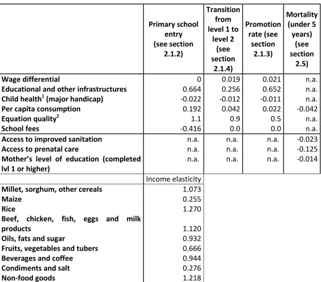
The elasticities of the MDGs (see section on the description of the model) and those on household consumption were estimated econometrically using the EICVM 2009 survey (see Table 1) following the approaches presented in detail in section 2. For elasticities related to trade and in the production function, we have taken the values used by Balma et al (2011). Table 1: Estimated elasticities
Primary school entry (see section 2.1.2) Transition from level 1 to level 2 (see section 2.1.4) Promotion rate (see section 2.1.3) Mortality (under 5 years) (see section 2.5)
Wage differential 0 0.019 0.021 n.a.
Educational and other infrastructures 0.664 0.256 0.652 n.a. Child health1 (major handicap) -0.022 -0.012 -0.011 n.a.
Per capita consumption 0.192 0.042 0.022 -0.042
Equation quality2 1.1 0.9 0.5 n.a.
School fees -0.416 0.0 0.0 n.a.
Access to improved sanitation n.a. n.a. n.a. -0.023 Access to prenatal care n.a. n.a. n.a. -0.125 Mother’s level of education (completed
lvl 1 or higher) n.a. n.a. n.a. -0.014
Income elasticity Millet, sorghum, other cereals 1.073
Maize 0.255
Rice 1.270
Beef, chicken, fish, eggs and milk
products 1.120
Oils, fats and sugar 0.932
Fruits, vegetables and tubers 0.666
Beverages and coffee 0.944
Condiments and salt 0.276
Non-food goods 1.218
Note: 1 At the macro level, we use MDG4 to proxy child health. The micro model estimates the elasticity of
19
4.3. Microeconomic analysis
Figure 1: Schema followed for estimation in the micro component (for example, at time t=1)
The above schema (figure 1) shows the procedure and the order followed in estimating the micro component of the model. The following methodological notes are presented in the same order. We begin with the analysis of the education sector, which also helps to define the new sample of skilled and unskilled individuals in time t=1,2,… As indicated in the schema, education in time t is assumed to be a function of consumption in time t-1. We then estimate the change in wage income in time t (we assume other sources of income are not affected by the simulated changes in education). After estimating the changes in income, we can predict the changes in real consumption in time t, which also depends on changes in consumer prices. The new vector of real consumption in time t ultimately influences child mortality and caloric consumption in time t. Finally, we use the new figures for the consumption vector and mortality in time t to estimate education in time t+1, which in turn determines the sample of skilled and unskilled workers in time t+1.
Before going into more detail about the subcomponents of the micro analysis, it is important to mention the demographic assumptions: the sample in the base year (the year of the household survey used in this study) is assumed to be constant across time and simulation scenarios. In other words, the age of individuals is held constant, as is household structure.
4.3.1. Education
Base models and estimation coefficients
The goal in this section is to estimate the behaviour of children with respect to entry into primary school, passing the first cycle of education, and the choice to enter the second cycle for
Education=f(X, Consumptiont-1)
ΔWageIncomet (estimated from samples of skilled and unskilled individuals after estimating Educationt=1) ΔConsumptiont = f(X, ΔWageIncomet, ΔOtherIncomet, ΔConsumerPricet) Educationt+1=f(X, Consumptiont, Mortalityt) ΔCaloriest = f(X, ΔConsumptiont) Mortalityt = f(X, ΔConsumptiont)
20 those who complete the first. Remember that the first cycle of education includes the primary school as well as the first four years of secondary school. The second cycle of education includes the three final years of secondary school as well as post-secondary education.
These models provide us with coefficients and elasticities to pass on to the macro model and allow us to identify the determinants of different education-related results, such as those presented above, and to exactly predict which children will be affected by the fiscal and social policies modelled in this study.
Entry to primary school
The probability of entering primary school is estimated from a sample of children aged 6-8 years using a probit model. Even though the legal age for school entry is 7 years, we also include those aged 6 years (because the survey only provides this information in years, with no information on month of birth) and those aged 8 years (because it is common in Burkina Faso for a child to delay school entry by a year). Among these children, only those who did not attend primary school in the previous year are retained.
( )
i v i iprobit
π
= +
α β
X
+
ε
With:(
)
iE Y X
i iπ
=
where Yi is a binary variable taking a value of 1 if the child attended the first year of primary
school in the survey year but not in the previous year, and 0 otherwise. The vector Xi includes
the V individual, household and community socioeconomic characteristics of child i. The explanatory variables introduced in this model specification are specific to the school entry model, and are: whether the child has a birth certificate, whether the child attended preschool, the number of children aged 6-8 (the age used to estimate primary school entry) in the same household, the distance between the primary school and the child’s residence and primary school fees. This last variable is introduced in order to estimate the price elasticity of demand (or better, of the average probability) to enter school and to provide important guidance to policy makers. They were constructed by taking the median value of school fees paid directly by households in each census zone.
Other explanatory variables that are common to the three education models are: sex of child, age (and age squared), urban/rural residence, education level of household head as well as his/her age group and sex, real per capita household consumption and whether the child suffers from a major handicap.
Completing the first cycle of education
As above, the probability of completing the first cycle of education is estimated using a probit model. To carry out this analysis, we take a sample of children up to the age of 25 inclusive who completed the final year of the first cycle in the previous year. Even if the expected age to obtain a diploma (Brevet d’Étude du Premier Cycle, BEPC) is 17, we opted for a sample that includes a larger age group because few people reach this level in Burkina Faso and because here we are not specifically interested in the child’s age upon graduation.
Yi is a binary variable taking a value of 1 if the child’s highest completed the first cycle of
21 addition to the explanatory variables included in all three of the education models, the variables which are specific to this model are distance to secondary school from where the child lives and the ratio between income earned by a skilled worker and that of an unskilled worker. This last variable was constructed using median values of skilled and unskilled workers in each census zone.
Continuation to the second cycle of education
The probability of continuing on to the second cycle is estimated with a probit model. To do this, we retained a sample of children aged 16-25 inclusive, with a CAP diploma or higher and who were not working.
Yi is a binary variable taking a value of 1 if the child attended class 2nde or higher and had
obtained a CAP diploma or higher, and is 0 otherwise. The explanatory variables are the same as in the model in the previous section.
Simulations
After estimating the coefficients, we replace the values for certain explanatory variables in the models presented in section 2.1.2 with their simulated values, and then predict the probability of entry into primary school. More specifically, real per capita consumption and school fees (this latter, for the entry model only) are replaced with the relevant (simulated) values.
In order to determine the change in primary school entry, the sample here (children aged 6-8 years) is then ordered with respect to the individual probability of entering primary school. We then use the predicted changes to assign a new status to the relevant children: for example, if the macro model predicts a 3% increase in the primary entry rate, we only change the variable
Yi to a value of 1 for the 3% of children who did not go to school in the base year and who had
the highest probability of entering school.
The newly skilled individuals are either those who graduated from the first cycle and do not continue their studies or who complete or drop out of their studies at the second cycle of education. They are chosen randomly from the appropriate sample (respectively among people who graduate and those who continue on to the second level of education) using simulated changes in the macro model for both cases. In these two cases, we do not have enough observations to use an econometrically estimated behavioural model to determine who enters the labour market.
4.3.2. Sources of income
The following sources of income are used in the micro model. The predicted changes, as well as consumption prices, ultimately influence child welfare, whether in terms of monetary or caloric consumption or in terms of education and health.
Wages
The analysis of the changes in employment status in the wage sector (which accounts for just 4.1% of workers) and of observed and potential wages is carried out on the sample of individuals aged 15-65 inclusive who work in the wage sector or who do not work at all. We thus assume that the other types of workers (self-employed workers, apprentices or domestic workers) are not eligible to work in the wage sector (otherwise stated, the model assumes intersectoral immobility). Two models are specified, one for each level of qualification (skilled or unskilled).
22 The equations used to estimate the wage rate in the skilled (q) and unskilled (nq) sectors are defined as follows:
ln
ln
q i q vq i i nq i nq vnq i iw
X
w
X
α
β
ε
λ
ϑ
υ
=
+
+
=
+
+
Where lnwiq and ln nq iw are the logarithms of wages earned by individual i, who is either skilled
or unskilled, as defined in the section on education. The first regression is estimated on the sample of individuals defined at the beginning of this section and who are skilled, while the second is estimated on unskilled individuals. The vector Xi includes the following explanatory
variables for individual i: sex of the individual, whether he/she is the household head, region of residence, age and age squared, and level of education and its square.
These equations are estimated using a standard Heckman-type selection model. When wage rates in a specific sector are only observed if the individual works in this sector, a selection problem arises. This is more of an issue when the error term in the wage equation is correlated to the error term in the equation which predicts the probability that the individual works in a given sector. In the presence of selection bias, the ordinary least squares estimators of the constant and the explanatory variables are biased and not consistent. The Heckman procedure provides consistent estimators and can estimate the wage equation in a sector under the condition that the individual actually works in the sector. Using maximum likelihood techniques, we jointly estimate the wage equations and the probability of employment (or selection) for both skilled and unskilled workers. The employment probability equation is estimated using the following explanatory variables: marital status of the individual, age and age squared, sex, education level, region of residence and the number of children living with him/her. The marital status and the number of children are necessary instruments to correct for selection problems. We then predict the wage rate and the probability of employment in the two sectors for each individual in the retained sample. The changes simulated by the macro model are then integrated into the micro component. More specifically, the individuals are ordered by their probability of being employed in one of two sectors. If there is an increase (decline) in the employment rate, then individuals with a higher (lower) probability and who do not work (work) in the relevant sector become workers (non-workers). Clearly, the analyzed samples (skilled and unskilled) must be updated at the beginning of each simulation scenario by importing the predicted status changes from the primary school pass model. Then, the change in the wage rate is applied to observed wages (or predicted for individuals who for some reason or another did not report their income). Finally, the changes in the wage sector are calculated at the per capita and household levels.
Self-employment
The per capita changes in income among the self-employed13 (34.4% of workers) are derived by applying the changes in the sectoral value added from the macro model (net of changes in labour demand). The sectors were classified following the categories in the input-output table. The income of individuals working as caregivers, apprentices/interns or volunteers (respectively 54.3%, 6.9 and 0.2% of workers) is assumed constant.
13 Among the self-employed, no response was given for income in about 40% of cases; these were replaced by estimated (region-specific) values using a Heckman selection model.