HAL Id: pastel-00755348
https://pastel.archives-ouvertes.fr/pastel-00755348
Submitted on 21 Nov 2012
HAL is a multi-disciplinary open access archive for the deposit and dissemination of sci-entific research documents, whether they are pub-lished or not. The documents may come from
L’archive ouverte pluridisciplinaire HAL, est destinée au dépôt et à la diffusion de documents scientifiques de niveau recherche, publiés ou non, émanant des établissements d’enseignement et de
sans GPS et autres exemples de conception de systèmes
de navigation MEMS
Pierre-Jean Bristeau
To cite this version:
Pierre-Jean Bristeau. Techniques d’estimation du déplacement d’un véhicule sans GPS et autres exemples de conception de systèmes de navigation MEMS. Automatique / Robotique. École Nationale Supérieure des Mines de Paris, 2011. Français. �pastel-00755348�
T
H
È
S
E
INSTITUT DES SCIENCES ET TECHNOLOGIES
École doctorale n
O432: Sciences des Métiers de l’Ingénieur (SMI)
Doctorat ParisTech
T H È S E
pour obtenir le grade de docteur délivré par
l’École Nationale Supérieure des Mines de Paris
Spécialité « Mathématique et Automatique »
présentée et soutenue publiquement par
Pierre-Jean BRISTEAU
le 6 décembre 2011
Techniques d’estimation du déplacement
d’un véhicule sans GPS
et autres exemples de conception
de systèmes de navigation MEMS
Directeur de thèse:Nicolas PETIT
Jury
M. Tarek HAMEL,Professeur, I3S, Université de Nice-Sophia-Antipolis Rapporteur M. Lorenzo MARCONI,Professeur, LAR-DEIS, Université de Bologne Rapporteur
M. Knut GRAICHEN,Professeur, IMRM, Université d’Ulm Examinateur
M. Vincent ANDRIEU,Chargé de recherche, LAGEP, CNRS Examinateur
M. Philippe MOUYON,Docteur, DCSD, ONERA Examinateur
M. Nicolas PETIT,Professeur, CAS, MINES ParisTech Examinateur
M. Xavier MICHÉ,Ingénieur, ST(SI)2 Invité
T
H
È
S
E
INSTITUT DES SCIENCES ET TECHNOLOGIES
Graduate School n
O432: Sciences des Métiers de l’Ingénieur (SMI)
ParisTech
P H D T H E S I S
To obtain the Doctor’s degree from
École Nationale Supérieure des Mines de Paris
Speciality « Mathématique et Automatique »
defended in public by
Pierre-Jean BRISTEAU
on December 6th, 2011
Motion estimation techniques
for GPS-free vehicle
and other examples
of MEMS navigation systems design
Thesis advisor:Nicolas PETIT
Committee
M. Tarek HAMEL,Professor, I3S, University of Nice-Sophia-Antipolis Reviewer
M. Lorenzo MARCONI,Professor, LAR-DEIS, University of Bologne Reviewer
M. Knut GRAICHEN,Professor, IMRM, University of Ulm Examiner
M. Vincent ANDRIEU,Chargé de recherche, LAGEP, CNRS Examiner
M. Philippe MOUYON,Doctor, DCSD, ONERA Examiner
M. Nicolas PETIT,Professor, CAS, MINES ParisTech Examiner
M. Xavier MICHÉ,Engineer, ST(SI)2 Invited
Centre Automatique et Systèmes Unité Mathématiques et Systèmes MINES ParisTech
60 boulevard St Michel 75272 Paris Cedex France.
E-mail: [email protected]
Key words. - GPS-free navigation systems, MEMS sensors, embedded systems, observability, Kalman filtering, interconnected observers, temporally interconnected observers, automotive vehicle, micro-UAV, mini-rocket
Mots clés. - systèmes de navigation sans GPS, capteurs MEMS, systèmes embarqués, observabilité, filtrage de Kalman, observateurs interconnectés, observateurs temporellement interconnectés, véhicule automobile, micro-drone, mini-fusée
La recherche doit avant tout être un jeu et un plaisir.
Pierre Joliot, La recherche passionnément, Ed. Odile Jacob.
L’esprit qui invente est toujours mécontent de ses progrès, parce qu’il voit au-delà.
Remerciements
Je remercie, en premier lieu, mon directeur de thèse, Nicolas Petit, qui m’a guidé et appuyé dans mes recherches, en me laissant à la fois une grande autonomie et en me proposant une grande diversité de sujets et d’activités.
Je remercie également David Vissière pour l’opportunité qu’il m’a donnée de travailler sur ce sujet aussi captivant que l’avait été un précédent stage à ses côtés, pour sa confiance et son soutien.
Je les remercie tous les deux de m’avoir associé à leur projet SYSNAV au sein duquel j’espère pouvoir continuer à travailler de manière fructueuse à leurs côtés.
Je suis reconnaissant envers messieurs Hamel et Marconi pour l’honneur qu’ils m’ont fait en acceptant d’être rapporteurs de cette thèse. Mes remerciements vont de même à messieurs Graichen, Andrieu et Mouyon pour leur présence dans mon jury.
Je remercie tout particulièrement Xavier Miché pour son accompagnement et son implication au cours de ma thèse et sa présence à ma soutenance.
J’adresse aussi mes remerciements à Philippe Martin pour ses discussions toujours animées et à Laurent Praly pour son aide précieuse.
Je ne saurais oublier mes " collègues " doctorants, en particulier, Erwan, Eric et Caroline ainsi que ceux que j’ai côtoyés lors de mes trois années au CAS, Mathieu, Thomas, Florent, Zakhi, Paul, Delphine, Hadis et Nadège. Je pense bien sûr également aux stagiaires que j’ai eu plaisir à encadrer.
Je remercie également mes " collègues de la première heure " Alain, Quentin et Yohann pour leur soutien technique toujours enthousiaste. Mes remerciements vont aussi à Manu, Nicolas et Lionel qui ont partagé avec moi quelques problématiques scientifiques.
Pour boucler la boucle, je remercie sincèrement Gaël Désilles qui m’a mis le pied à l’étrier dans ce milieu passionnant que forment la navigation et les personnes qui le constituent.
Bien sûr, je tiens à remercier ma famille et mes amis, souvent intéressés, parfois intrigués mais toujours présents à mes côtés.
Enfin, je tiens à remercier, sur un plan plus personnel, Nicolas pour ces années passées à ses côtés, depuis un entretien (en béquilles) pour un stage jusqu’à l’obtention de cette thèse. M’investir dans cette thèse fut un plaisir et cela tient pour beaucoup à son humanité et à sa façon d’animer le CAS, parfaitement illustrée par les citations en page précédente.
Motion estimation techniques
for GPS-free vehicle
and other examples
Résumé
Dans cette thèse, on explique la conception et la mise au point d’un système de navigation sans GPS pour un véhicule automobile. Ce système exploite des mesures de champs magnétiques réalisées à bord du véhicule en mouvement, combinées à des mesures inertielles réalisées à partir de capteurs MEMS bas coût. Il permet de reconstituer, à partir d’une condition initiale, la trajectoire du véhicule en temps réel. Un prototype fonctionnel complet est présenté ainsi que des résultats expérimentaux. La conception de ce système repose sur une analyse de l’observabilité d’un modèle classique du véhicule, qui permet d’établir comment les différents biais et défauts des capteurs peuvent être estimés grâce à des filtres de Kalman agencés suivant deux schémas d’interconnexion: par partition des variables d’états et par séquencement. Une analyse de convergence des schémas d’estimation est étudiée. En dernière partie du manuscrit, deux autres exemples de systèmes de navigation à base de capteurs MEMS sont décrits, celui du quadricoptère Parrot AR.Drone et celui de fusées expérimentales à propulsion hybride, pour lesquels les mêmes principes de conception sont appliqués.
Abstract
In this thesis, we explain the design and development of a GPS-free navigation system for automotive vehicles. This system uses magnetic field measurements performed onboard the vehicle in motion, and combines them with inertial measurements from other low costs MEMS sensors. It allows one to reconstruct the path of the vehicle from the initial condition in real time. A complete prototype is presented along with experimental results. The design of this system is based on an analysis of the observability of a classical model of the vehicle. This serves to establish how the various biases and shortcomings of the sensors can be estimated through Kalman filters arranged in two interconnection schemes: a partition of the state variables and a temporal interconnection. An analysis of convergence of the estimates is performed. In the final part of the manuscript, two other examples of MEMS-based navigation systems are described, including the AR.Drone quadrotor and experimental hybrid rockets for which the same design principles are applied.
Contents
Introduction 1
1 Notations 3
1.1 Frames of reference and parametrization of orientation . . . 3
1.2 Euler angles . . . 4
1.3 Quaternions . . . 4
1.4 States, dynamics and measurement . . . 6
Acronyms 9 I Kalman filtering and observability 11 2 A quick tour of Kalman filtering 15 2.1 Kalman-Bucy filter . . . 15
2.2 Extended Kalman filter . . . 19
2.3 Discrete-time Kalman filter . . . 20
2.3.1 Sampled Linear-Time-Invariant system . . . 21
2.3.2 Mixed continuous-discrete-time filtering . . . 22
2.3.3 Multi-rates Kalman filter . . . 23
2.3.4 Remarks on the units . . . 24
2.4 Computational burden and numerical accuracy . . . 24
2.4.1 Sequential processing . . . 24
2.4.2 Joseph form . . . 25
2.4.3 Information filter . . . 25
2.4.4 Square-root filter . . . 26
3 Observability properties and their roles in the convergence of Kalman filters 27 3.1 Uniform and Complete Observability . . . 27
3.2 Differential Observability . . . 28
3.3 Existence and convergence of the Kalman filter . . . 32
3.3.1 Lower bound on the solution of the covariance equation from boundedness of the system . . . 33
3.3.2 Upper bound stemming from the Uniform and Complete Observability
property . . . 34
3.3.3 Convergence of the Kalman filter . . . 36
3.3.4 Estimation of the convergence rate . . . 37
3.4 Conclusion and main result . . . 38
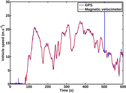
II GPS-free automotive relative navigation system 39 4 Exploitation of magnetic measurements onboard a vehicle 43 4.1 Magnetic velocimeter . . . 44
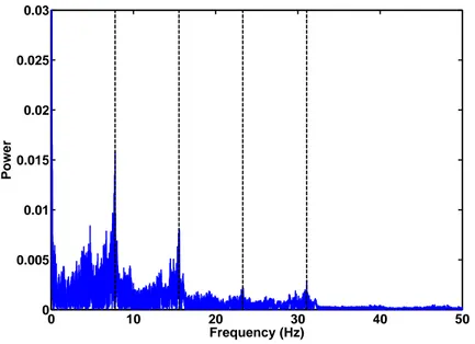
4.1.1 Frequency detection . . . 45
4.1.2 Stops detection . . . 47
4.1.3 Phase detection . . . 48
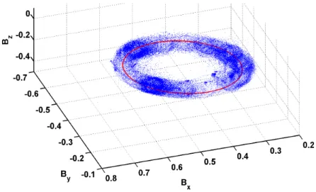
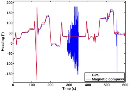
4.2 Magnetic heading determination . . . 49
4.2.1 Hard iron / soft iron distortions . . . 50
4.2.2 Ellipse detection . . . 51
4.2.3 Complementary filter . . . 54
5 Description of the relative navigation problem 55 5.1 Vehicle model under consideration . . . 55
5.2 Embedded sensors . . . 57
5.3 A view of practical issues . . . 58
6 Design of the navigation system 61 6.1 Observer design . . . 61
6.1.1 Interconnected subsystems . . . 61
6.1.2 Decomposition into Temporally Interconnected Observers . . . 65
6.2 Observability for the models used in the Temporally Interconnected Observers . . 68
6.2.1 Uniform and Complete Observability of the straight-line motion model . . 68
6.2.2 Differential Observability of the curve motion model . . . 68
6.3 Convergence of the Temporally Interconnected Observers structure . . . 73
7 Practical implementation and experimental results 79 7.1 Implementation of Kalman filtering . . . 79
7.2 On-line alignment procedure . . . 81
7.3 Numerical rate of convergence estimates . . . 83
7.4 Fault detection strategy . . . 83
7.5 Optimal smoothing for multi-rates filtering and a posteriori trajectory smoothing 85 7.6 Results . . . 87
7.6.1 Simulation illustrating biases estimation properties . . . 87
7.6.2 Short range experimental real-time reconstruction . . . 90
CONTENTS
III Other examples of navigation system design 95
8 The navigation problem aboard the AR.Drone 97
8.1 Navigation problem . . . 99
8.2 Aerodynamics modeling . . . 100
8.2.1 Method to calculate aerodynamics effects . . . 101
8.2.2 Dynamic coupling between the vehicle and the rotors . . . 104
8.3 Observer design and presentation of results . . . 107
9 A navigation problem for an experimental mini-rocket 115 9.1 The rocket under consideration . . . 116
9.1.1 Model . . . 116
9.1.2 Onboard instrumentation . . . 118
9.2 Trajectory estimation . . . 118
9.2.1 A typical trajectory . . . 118
9.2.2 Estimation technique . . . 119
9.2.3 Results exploiting in-flight measurements . . . 120
9.3 Estimation of propulsion parameters . . . 122
9.3.1 Combustion system measurements . . . 123
9.3.2 Thrust model of hybrid engine . . . 123
9.3.3 Results exploiting in-flight measurements . . . 124
9.4 Conclusion . . . 126
Conclusion 129 Appendix 133 A Discussion on the smoothing technique: a comparison with back-and-forth filtering on simple examples 135 A.1 Cramér-Rao bound for a biased estimator . . . 136
A.2 Identification of a constant . . . 138
A.2.1 Back-and-Forth Nudging . . . 139
A.2.2 Back-and-Forth Kalman filtering . . . 141
A.2.3 Mean estimator . . . 142
A.3 Estimation of a first-order dynamics . . . 145
A.3.1 Back-and-Forth Nudging . . . 145
A.3.2 Back-and-Forth Kalman Filtering . . . 146 B The role of the location of the center of gravity in quadrotor stability 151
Introduction
In this thesis, we expose the principles of a navigation system that we have created for automotive applications. It consists of embedded Micro-Electro-Mechanical Systems (MEMS) sensors and allows one to estimate the position and the orientation, relative to initial conditions, of an automotive vehicle. The major feature of this system is that it does not use any Global Positioning System (GPS) receiver.
This thesis describes the scientific steps that have been necessary to design a functional prototype. This design relies on the observability properties of the vehicle dynamics model when it is equipped with a particular set of sensors. The fundamental principles employed to estimate the vehicle motion stem from the theory of inertial navigation. Classically, when high quality (tactical grade) inertial sensors (accelerometers and gyrometers) are used, their signals can be integrated once then twice to obtain, sequentially, attitudes, velocities and position estimates. In this thesis, we consider low-cost MEMS sensors. Their numerous defects, among which are non negligible biases, discard the classic technique previously mentioned. In particular, the biases generate overwhelming drift in the integrations producing the estimates. Other solutions must be found.
Onboard the vehicle, we embed MEMS accelerometers, gyrometers along with magnetometers and a barometric altitude sensor. A particularity of our approach is that the magnetometers are used to measure the ground velocity and the heading of the vehicle. The relative redundancy of the sensors measurements is analyzed through careful investigations on observability. In details, it is shown that all the variables needed to estimate the relative motion of the vehicle can be reconstructed. The model under consideration is a simple six degrees of freedom (6-DOF) rigid body dynamics, in constant contact with the road, without slip. The sensors are modeled according to classic error models incorporating biases. A main contribution of the thesis is to show the reconstructibility of the dynamics state vector in this context. We now explain how this study is organized.
Usually, reconstructibility can be conveniently established by invoking a classic Kalman filter (as recalled in Chapter 2) which asymptotic convergence is guaranteed under the Uniform and Complete Observability (UCO) property (recalled in Section 3.1). This point is exposed in details in Section 3.3. Formally, the UCO property is difficult to establish. Much more conveniently, we propose to relate it to an easily checkable rank test of Differential Observability (DO) as is exposed in Section 3.2. A result of Chapter 3 is that DO implies UCO which, in turn, implies convergence of Kalman filtering. This result guides us in the design of the navigation system.
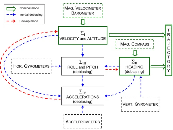
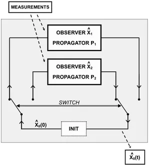
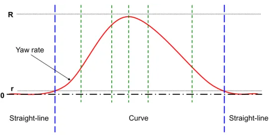
sensors data come into play in a way depending on the (a priori unknown) nature of the vehicle trajectory. In details, the malicious effects of vehicle braking on the magnetometer information, and the interaction of rotations, translations, and slopes on gyrometric data are detailed in Chapter 5. In the navigation filter, we split the state variables into subsets. This allows us to isolate the effects of each sensor bias. During favorable sequences, the bias are estimated. Then, the estimates can be used to handle the discussed malicious effects. Bias estimation is relatively straightforward for accelerometers but the situation is much more involved for gyrometers. The natural couplings of axes due to the Euler angles parametrization (recalled in Section 1.2) suggest to isolate the yaw angle and the corresponding bias. On the other hand, the roll and pitch angles and the corresponding gyrometers biases must be estimated jointly. All these considerations yield us to introduce a structure of interconnected observers detailed in Section 6.1.1. At the center of the interconnection is the roll-pitch subdynamics. It is the subject of Chapter 6.1.2. Globally, this sub-dynamics is not observable. The variables can not be simultaneously observed, but the observability deficiency corresponds to a different variable depending on the nature of the trajectory currently followed by the vehicle. For this reason, the roll-pitch dynamics is observed using three Temporally Interconnected Observers (TIO). The introduction of this class of observers is also a contribution of the thesis. At each instant, only one of the TIO is processing measurements, the others being updated (propagated) in open loop. The TIO constitute a set of separately contracting then propagating dynamics. In the case under consideration, convergence of the TIO scheme is proved. This is the contribution of Section 6.3.
Numerous field experiments have been conducted and a selection of them, along with details of implementation, are reported in Chapter 7. It appears that, in urban or countryside experiments, over periods ranging from several hours to days, for traveled distances of 1 km to 600 km, the actual motion of the vehicle can be reconstructed relatively accurately. The error between the position reconstructed from perfect initial conditions and the actual position of the vehicle is below 10% of the traveled distance, more often that not below 5%.
The rest of the manuscript is dedicated to other examples of navigation filter design. Chapter 8 describes the attitude and velocity data fusion algorithms embedded in the AR.Drone (Parrot©). As is exposed, it relies on a tight coupling of inertial sensors and camera streams. This navigation system is the heart of this popular autonomous Unmanned Aerial Vehicle (UAV). Chapter 9 reports trajectory estimation results for experimental mini-rockets operated by Centre National d’Etudes Spatiales, National Center for Space Research (CNES). Off-line processing of embedded sensors serve to quantify the engine efficiency. In both cases, the employed navigation techniques are discussed at the light of the observability-based design advocated in this thesis.
Chapter 1
Notations
Notations
Ce chapitre introduit les notations générales utilisées ultérieurement dans cette thèse. Les repères de référence y sont détaillés ainsi que deux façons de déterminer leurs orientations res-pectives. Les variables dynamiques sont présentées sous leur forme vectorielle et en composantes scalaires.
1.1
Frames of reference and parametrization of orientation
For each application considered in this thesis, a Galilean frame of reference is considered. This (local) inertial frame is noted Ri = (xi, yi, zi) and is oriented using the North-East-Down formalism, the ziaxis being aligned with the gravity direction, the xiaxis with the local meridian and the yi axis with the local parallel, respectively. Its origin is Oi. Earth rotation, Earth curvature and local variations of gravity are neglected.
A body frame Rb = (xb, yb, zb) is associated to the vehicle under consideration. Its origin Ob is the center of gravity of the vehicle. The xb axis is taken aligned with the longitudinal axis of the vehicle, the zbis directed downward such that the plane(xb, zb) is a symmetry plane for the vehicle, and, finally, the yb axis completes the direct frame. The orientation of the body frame compared to the inertial frame is given by three successive rotations described in Fig. 1.1. From the inertial frame, the first rotation, of angle ψ, is around the zi axis, the second rotation, of angle θ, is around the intermediate y1 axis and finally the third rotation, of angle φ, is around the xb axis.
This choice of rotations is one possibility among various Euler angles combinations (here a ZYX combination). It corresponds to angles used in aeronautics [Titterton and Weston, 2004], where the ψ-angle is named yaw angle (or heading angle), the θ-angle is the pitch angle and the φ-angle is the roll angle.
(a) Yaw (b) Pitch (c) Roll Figure 1.1: Orientation of the Rb frame with respect to the Ri frame.
The change of coordinates from Ri to Rbcan be expressed in terms of the Euler angles under the form of the following matrix
PRi→Rb = ⎛ ⎜ ⎝ cθcψ cθsψ −sθ sφsθcψ− cφsψ sφsθsψ+ cφcψ sφcθ cφsθcψ+ sφsψ cφsθsψ− sφcψ cφcθ ⎞ ⎟ ⎠ (1.1)
where cθ= cos θ and sψ = sin ψ, e.g.
1.2
Euler angles
The rotation of Rbwith respect to Riis described by the rotation vector Ω whose components, when expressed in the body frame are the roll rate p, the pitch rate q and the yaw rate r. In vector notations, one has
Ω= pxb+ qyb+ rzb = ˙ψzi+ ˙θy1+ ˙φxb
= ( ˙φ − ˙ψsθ) xb+ ( ˙θcφ+ ˙ψsφcθ) yb+ ( ˙ψcφcθ− ˙θsφ) zb
(1.2) The sequence of rotations pictured in Fig. 1.1 introduces coupling between the angles dynamics. The rotation components in the body frame, (p, q, r) are different from the angles derivatives( ˙φ, ˙θ, ˙ψ). One-to-one correspondence relations are given below
⎧⎪⎪⎪ ⎨⎪⎪⎪ ⎩ p= ˙φ − ˙ψsθ q= ˙θcφ+ ˙ψsφcθ r= ˙ψcφcθ− ˙θsφ ⎧⎪⎪⎪ ⎪⎪⎪ ⎨⎪⎪⎪ ⎪⎪⎪⎩ ˙ ψ= sφq+ cφr cθ ˙ θ= cφq− sφr ˙ φ= p + (sφq+ cφr) sθ cθ
1.3
Quaternions
Depending on the considered application, the singularity encountered by the Euler angles around θ = ±π/2 can reveal more or less troublesome. Simply, quaternions can be introduced
1.3. QUATERNIONS
to circumvent it. The quaternion describes the orientation of Rb with respect to Ri by a three-dimensional vector and a rotation around this vector. Naturally, this leads a four parameters representation. To obtain uniqueness of the description, the quaternion is normalized.
In summary, a quaternionQ is a quadruplet (q0, q1, q2, q3) constrained by q02+ q12+ q22+ q32= 1 Q = ⎡⎢ ⎢⎢ ⎢⎢ ⎢⎢ ⎣ q0 q1 q2 q3 ⎤⎥ ⎥⎥ ⎥⎥ ⎥⎥ ⎦ △ = ⎡⎢ ⎢⎢ ⎢⎢ ⎢⎢ ⎣ cos µ/2 µx/µ sin µ/2 µy/µ sin µ/2 µz/µ sin µ/2 ⎤⎥ ⎥⎥ ⎥⎥ ⎥⎥ ⎦
where µx, µy, µz can be interpreted as the components of the mentioned vector and µ defines the rotation angle.
The time derivative of the quaternion is bilinear and can be written under either of the following two convenient forms
˙ Q = 1 2 ⎛ ⎜⎜ ⎜ ⎝ 0 −p −q −r p 0 r −q q −r 0 p r q −p 0 ⎞ ⎟⎟ ⎟ ⎠ Q = 1 2 ⎛ ⎜⎜ ⎜ ⎝ q0 −q1 −q2 −q3 q1 q0 −q3 −q2 q2 q3 q0 −q1 q3 −q2 q1 q0 ⎞ ⎟⎟ ⎟ ⎠ ⎡⎢ ⎢⎢ ⎢⎢ ⎢⎢ ⎣ 0 p q r ⎤⎥ ⎥⎥ ⎥⎥ ⎥⎥ ⎦
In application, it is often necessary to implement the discrete-time version of the preceding differential equation. In a numerical scheme, additive integration scheme presented below in Eq. (1.3) preserves the norm. But, the usually considered normalization step can introduce significant errors when the discretization step is too large compared to the bandwidth of the dynamics of(p, q, r).
{ Q(t) = Q(t) + ˙Q(t)∆tQ(t + ∆t) = ˜˜ Q(t)/∣∣ ˜Q(t)∣∣ (1.3) In such cases, multiplicative integration can be preferred despite its increased computational burden. It takes the form, which will be used in Chapter 9,
⎧⎪⎪⎪ ⎪⎪⎪⎪⎪ ⎪⎪⎪⎪⎪ ⎨⎪⎪⎪ ⎪⎪⎪⎪⎪ ⎪⎪⎪⎪⎪ ⎩ α(t) = ∆t∣∣Ω(t)∣∣, n(t) =⎡⎢⎢⎢ ⎢⎢ ⎣ p q r ⎤⎥ ⎥⎥ ⎥⎥ ⎦ /∣∣Ω(t)∣∣, ˜Q(t) = [n(t) sin α(t)/2]cos α(t)/2 Q(t + ∆t) = ⎛ ⎜⎜ ⎜ ⎝ q0 −q1 −q2 −q3 q1 q0 q3 −q2 q2 −q3 q0 q1 q3 q2 −q1 q0 ⎞ ⎟⎟ ⎟ ⎠ (t) ˜Q(t)
Finally, the one-to-one correspondence between Euler angles and quaternions is given below. ⎧⎪⎪⎪ ⎪⎪⎪⎪⎪ ⎪⎪⎪⎪ ⎨⎪⎪⎪ ⎪⎪⎪⎪⎪ ⎪⎪⎪⎪ ⎩ q0= cos φ 2 cos θ 2cos ψ 2 + sin φ 2sin θ 2sin ψ 2 q1= sin φ 2cos θ 2cos ψ 2 − cos φ 2sin θ 2sin ψ 2 q2= cos φ 2 sin θ 2cos ψ 2 + sin φ 2cos θ 2sin ψ 2 q3= − cos φ 2cos θ 2sin ψ 2 + sin φ 2sin θ 2cos ψ 2 ⎧⎪⎪⎪ ⎪⎪⎪⎪⎪ ⎨⎪⎪⎪ ⎪⎪⎪⎪⎪ ⎩ φ= arctan 2(q2q3+ q0q1) q02− q12− q22+ q32 θ= arcsin −2(q1q3− q0q2) ψ= arctan 2(q1q2+ q0q3) q2 0+ q21− q22− q32
The change of coordinates matrix (1.1) can also be expressed in terms of quaternion. PRi→Rb = ⎛ ⎜ ⎝ q02+ q21− q22− q32 2(q1q2+ q0q3) 2(q1q3− q0q2) 2(q1q2− q0q3) q02+ q22− q21− q32 2(q2q3+ q0q1) 2(q1q3+ q0q2) 2(q2q3− q0q1) q02+ q32− q21− q22 ⎞ ⎟ ⎠
1.4
States, dynamics and measurement
From the preceding, orientation of the body frame is given by the triplet (φ, θ, ψ) or equivalently by the (normalized) quaternion (q0, q1, q2, q3). The components of the rotation vector Ω of the body frame Rb with respect to the inertial frame Ri, expressed in the body frame Rb, are denoted by (p, q, r). The change of coordinates matrix, from the inertial frame to the body frame, noted PRi→Rb, satisfies
d
dtPRi→Rb = −Ω ∧ PRi→Rb
The position of the rigid body defined by the position of its center of mass Ob with respect to the origin Oi of the reference frame Ri expressed in the inertial frame is given by (x, y, z). The velocity V relative to the inertial frame is expressed by (u,v,w) in Rb coordinates and by (vx,vy,vz) in Ri coordinates, it satisfies the vector definition
dOiOb dt ∣Ri
= V which, once projected onto Rb, gives
d dt ⎡⎢ ⎢⎢ ⎢⎢ ⎣ x y z ⎤⎥ ⎥⎥ ⎥⎥ ⎦ =⎡⎢⎢⎢⎢⎢ ⎣ vx vy vz ⎤⎥ ⎥⎥ ⎥⎥ ⎦ = PRb→Ri ⎡⎢ ⎢⎢ ⎢⎢ ⎣ u v w ⎤⎥ ⎥⎥ ⎥⎥ ⎦
The acceleration Γ of the rigid body relative to the inertial frame expressed in the body frame is (Γx,Γy,Γz). One has
dV dt ∣Rb
= dV dt ∣Ri
− Ω ∧ V = Γ − Ω ∧ V which, once projected onto Rb, gives
d dt ⎡⎢ ⎢⎢ ⎢⎢ ⎣ u v w ⎤⎥ ⎥⎥ ⎥⎥ ⎦ =⎡⎢⎢⎢⎢⎢ ⎣ Γx Γy Γz ⎤⎥ ⎥⎥ ⎥⎥ ⎦ −⎡⎢⎢⎢⎢⎢ ⎣ p q r ⎤⎥ ⎥⎥ ⎥⎥ ⎦ ∧⎡⎢⎢⎢⎢⎢ ⎣ u v w ⎤⎥ ⎥⎥ ⎥⎥ ⎦
Unless otherwise specified, the sensor frame is the same as the body frame and the measurements inherit the subscript m. For example, the gyrometers give the measurement vector Ωm = [pm qm rm]
T
1.4. STATES, DYNAMICS AND MEASUREMENT
Γm= [axm ay m az m] T
which are the measurements of[ax ay az] T
. In case perfect sensors are considered (noise and biases being neglected), it yields
Ωm= Ω, Γm = Γ − PRi→Rb ⎡⎢ ⎢⎢ ⎢⎢ ⎣ 0 0 g ⎤⎥ ⎥⎥ ⎥⎥ ⎦ d dt ⎡⎢ ⎢⎢ ⎢⎢ ⎣ u v w ⎤⎥ ⎥⎥ ⎥⎥ ⎦ =⎡⎢⎢⎢⎢⎢ ⎣ axm ay m az m ⎤⎥ ⎥⎥ ⎥⎥ ⎦ + g⎡⎢⎢⎢⎢⎢ ⎣ −sθ sφcθ cφcθ ⎤⎥ ⎥⎥ ⎥⎥ ⎦ −⎡⎢⎢⎢⎢⎢ ⎣ pm qm rm ⎤⎥ ⎥⎥ ⎥⎥ ⎦ ∧⎡⎢⎢⎢⎢⎢ ⎣ u v w ⎤⎥ ⎥⎥ ⎥⎥ ⎦ where g stands for the gravity and equals 9.81 m.s−2.
Depending on the application under consideration, position, velocity, angles and angular rates are gathered in the vector X with potentially other interesting states, for example, aerodynamics states or biases. In the case when (known) controls appear in the dynamics, they are represented by the vector U. All the measurements are assembled in the vector Y . The dimension of the state X (respectively the measurement Y ) is noted n (resp. m). The time-varying dynamics are written in state-space form as
Acronyms
6-DOF six degrees of freedom.
AEKF Adaptive High Gain Extended Kalman Filter. BFN Back-and-Forth Nudging.
CNES Centre National d’Etudes Spatiales, National Center for Space Research. CO Complete Observability.
DKF Distributed Kalman Filter. DO Differential Observability. EKF Extended Kalman Filter. FFT Fast Fourier Transform. GPS Global Positioning System.
HEKF Hybrid Extended Kalman Filter. HGEKF High Gain Extended Kalman Filter. IEKF Invariant Extended Kalman Filter. IEKF Iterated Extended Kalman Filter. IF Information Filter.
IGRF International Geomagnetic Reference Field. IMU Inertial Measurement Unit.
ISA International Standard Atmosphere. LCD Light Crystal Display.
LTI Linear-Time-Invariant. LTV Linear-Time-Varying.
MEMS Micro-Electro-Mechanical Systems.
ONERA Office National d’Etudes et de Recherches Aerospatiales, French Aerospace Lab. PDA Pitch Determination Algorithm.
PERSEUS project Projet Etudiant de Recherche Spatiale Européen Universitaire et Scien-tifique, European Student Project on Academic and Scientific Space Research.
PKF Pseudo Kalman Filter. PSD Power Spectral Density.
SR-IF Square-Root Information Filter.
SR-UKF Square-Root Unscented Kalman Filter. TIO Temporally Interconnected Observers. UAV Unmanned Aerial Vehicle.
UCE Uniform and Complete Estimatability. UCO Uniform and Complete Observability. UKF Unscented Kalman Filter.
UO Uniform Observability. ZUPT Zero velocity Update.
Part I
Kalman filtering and observability
Introduction
This part of the thesis contains a short exposition of Kalman filtering theory and related discussions on observability properties. The subject is well-established. In 1974, T. Kailath already proposed “a view of three decades of linear filtering theory” in a celebrated article [Kailath, 1974]. Thirty-seven years later, we propose a shortened view which clearly does not claim to be as exhaustive as the cited survey work, but simply aims only at highlighting key elements used in this thesis by situating the Kalman filter in the filtering theory. We gather here some well-known results on filtering, along with implementation considerations.
Optimal estimation problem treated from a stochastic point of view can be traced back to the pioneering works of Kolmogorov and Wiener. In the 1940s, Kolmogorov [Kolmogorov, 1941] and Wiener [Wiener, 1942] worked simultaneously on the question of a posteriori optimal estimation, which concerned the combination of knowledges on statistics in time series with needs at that time in communication engineering. Their seminal works announced the numerous future research efforts to find optimal filter in the sense of minimization of the stochastic parameters of error estimation. At this early time, the Wiener filter was dealing only with stationary processes. Estimation was realized a posteriori considering knowledge of all past values of the signal, with a filter design aiming at finding the filter impulse response minimizing the root mean square error covariance. We now sketch the philosophy of the method. The interested reader will find all the necessary details in [Van Trees, 1968].
Consider a signal a(t) of covariance function κa(t, u), corrupted by a noise n(t) with covariance κn(t, u). The objective is to find the filter impulse response t ↦ h(t) which provides the “best” estimate ˆa(t) from the measurement r(t) = a(t) + n(t) having the covariance function κr(t, u) = κa(t, u) + κn(t, u) + 2κan(t, u). Optimality is formulated as the minimization problem
min h E[ 1 T ∫ T 0 (a(t) − ˆa(t)) 2 dt] with ˆ a(t) = ∫ t 0 h(t, u)r(u)du
The corresponding necessary and sufficient condition for optimality is the following κar(t, u) = ∫
T
0 h(t, v)κr(u, v)dv, 0 ≤ t ≤ T, 0 < u < T
where κar(t, u) is the cross-covariance function between the signal to estimate, a(t) and the measurement r(t) (equal to κa(t) if the signal and the noise are uncorrelated)
Wiener filtering treats stationary processes with knowledge of infinite past. Then, the optimal filter satisfies the following equation known as the Wiener-Hopf equation
κar(τ) = ∫ ∞
0 h(ν)κr(τ − ν)dν, 0 < τ < ∞
Continuous and discrete solutions of this equation are presented in [Levinson, 1947, Wiener, 1949, Van Trees, 1968]. Early in the works of Wiener, it became evident that the
relaxed to form another problem. For non-stationary problems, assuming that observations were known only over a finite time interval in the past, a theory emerged under the well known name of Kalman-Bucy filtering or Kalman filtering [Kalman, 1960b, Kalman and Bucy, 1961].
In the applications treated in this thesis, the Kalman filtering will be our main tool for embedded data fusion. In Chapter 2, we expose this technique. In Chapter 3, we make a connection with the observability properties and establish a result guaranteeing the convergence of Kalman filter using an easy to check differential observability condition (Theorem 10). These are the main contributions of this part.
Chapter 2 focuses on the Kalman filter and its different forms and implementations. The condition of convergence being well known for Linear-Time-Invariant (LTI) dynamics, Chapter 3 is dedicated to the observability property sufficient for exponential convergence of Kalman filter for Linear-Time-Varying (LTV) dynamics.
Chapter 2
A quick tour of Kalman filtering
Un rapide panorama sur le filtrage de Kalman
Ce chapitre rappelle les éléments-clefs du filtre de Kalman. La version continue de Kalman-Bucy est utilisée afin de mettre en évidence les grandes lignes pour établir l’optimalité du filtre de Kalman. Outre la version étendue du filtre, la version discrète est également détaillée avec les différentes problématiques de discrétisation et de multi-échantillonnage afférentes. Enfin, plusieurs développements visant à réduire d’une part la charge de calcul et, d’autre part, à améliorer la précision numérique sont présentés.
2.1
Kalman-Bucy filter
In the 1960s, Kalman [Kalman, 1960b] and Bucy [Kalman and Bucy, 1961] worked, first separately and then together, to derive a filter which is optimal in the sense of minimization of the covariance of the error estimation. It has the advantage of offering the possibility to deal with many more types of processes than the Wiener filter thanks to the introduction of a dynamic process model and, very importantly, it can be implemented in real time as data are treated as they become available. Historically, the continuous-time formulation of the Kalman filter is not the first which has emerged but, compared to the discrete-time version, it is relatively simpler to understand, and, interestingly, easier and shorter to derive. This is why the discrete-time Kalman filter is only presented later in this chapter, along with its different implementations.
The Kalman filter is an adaptive optimal filter for a LTV system described by a dynamic process model involving dynamics noise (or disturbance input) and an observation equation corrupted with noise. In the following, the matrices A(t), B(t), C(t) are analytic.
The dynamics noise w(t) is a white, zero-mean Gaussian continuous random process1 of Power Spectral Density (PSD) matrix Q(t) which is symmetric definite positive
{ EE[w(t)] = 0[w(t)wT(τ)] = Q(t)δ(t − τ) (2.2) where δ(t − τ) is the Dirac function.
The measurement noise v(t) is a white, zero-mean Gaussian continuous random process of PSD matrix R(t) which is symmetric definite positive.
{ EE[v(t)] = 0[v(t)vT(τ)] = R(t)δ(t − τ) (2.3) The PSD matrix R(t) is taken definite positive even if singularity can be handled, see [Faurre, 1971, Gelb, 1974]. The noises are assumed white and zero-mean without loss of generality since biases and Markovian representation of coloration can be added to the state. Dynamics noises and measurement noises are assumed uncorrelated (their correlation is addressed in [Van Trees, 1968, Faurre, 1971, Gelb, 1974]).
E[w(t)vT(τ)] = 0 (2.4)
The expected value and the covariance of the initial state are used to initialize the observer. ⎧⎪⎪ ⎨⎪⎪ ⎩ ˆ X0 △ = E[X(0)] P0 △ = E[(X(0) − ˆX0)(X(0) − ˆX0)T] (2.5) Theorem 1(Kalman filter). The unbiased optimal filter of system (2.1) in the sense of minimum covariance matrix P is given by the observer ˆX, a.k.a. Kalman filter, computed with the Kalman gain K(t), obtained from the covariance equation (or differential Riccati equation), initialized using Eq. (2.5). ⎧⎪⎪⎪ ⎪⎨ ⎪⎪⎪⎪ ⎩ ˙ˆ
X(t) = A(t) ˆX(t) + B(t)U(t) + K(t)(Y (t) − C(t) ˆX(t)) K(t) = P(t)CT(t)R−1(t)
˙
P(t) = A(t)P(t) + P(t)AT(t) + Q(t) − P(t)CT(t)R−1(t)C(t)P(t)
(2.6)
The first equation can be interpreted as a combination of propagation, from the term found in the right-hand-side of (2.1)
A(t) ˆX(t) + B(t)U(t)
1. A white continuous random process is a mathematical object without physical realization since its energy is infinite. It can only be considered through a filter which limits the bandwidth of the process. The dynamic process model is a stochastic differential equation and should be formally considered by the yardstick of Itô integral or Stratonovich integral (see [Jazwinski, 1970]).
2.1. KALMAN-BUCY FILTER
and update (or correction), using the difference between the measurements and the predicted value of the measurements (called innovation)
+K(t)(Y (t) − C(t) ˆX(t))
Similarly, the third equation combines the propagation of the covariance due to the dynamics and the modeling uncertainties2
A(t)P(t) + P(t)AT(t) + Q(t) with the correction supplied by the measurement,
−P(t)CT(t)R−1(t)C(t)P(t)
Proof of existence of such an observer (in the sense of definition of ˆXand P for all times) will be detailed in Chapter 3.3. For simplicity, the spirit of the proof of optimality [Alazard, 2006] is given here in the time-invariant case, that is to say the matrices A, B, C, M, Q and R are constant. Time-varying proofs are given in [Van Trees, 1968, Bucy and Joseph, 1968, Jazwinski, 1970, Gelb, 1974, Stengel, 1994].
Proof. The linear time-invariant system is
{ XY˙(t) = CX(t) + v(t)(t) = AX(t) + BU(t) + w(t) The filter is of the following form
˙ˆ
X(t) = Af(t) ˆX(t) + Bf(t)U(t) + Kf(t)Y (t) Note ˜X(t) the estimation error, ˜X(t) = X(t) − ˆX(t)
˙˜
X(t) = AX(t) + BU(t) + w(t) − Af(t) ˆX(t) − Bf(t)U(t) − Kf(t)(CX(t) + v(t)) = (A − Kf(t)C)X(t) − Af(t) ˆX(t) + (B − Bf(t))U(t) + w(t) − Kf(t)v(t) = ∣ (A− Kf(t)C) ˜X(t) + (A − Kf(t)C − Af(t)) ˆX(t)
+(B − Bf(t))U(t) + w(t) − Kf(t)v(t) (2.7)
The input U being deterministic and the measurement Y being Gaussian, the observer ˆX is a Gaussian random variable (such as the state X). The Kalman filter has to be unbiased and shall provide minimal variance. The expected value of the error estimation is
d
dt(E( ˜X)(t)) = E( ˙˜X(t)) = ∣ (
A− Kf(t)C)E( ˜X(t)) + (A − Kf(t)C − Af(t))E( ˆX(t)) +(B − Bf(t))U(t)
2. If U contains an additive noise characterized by the PSD matrix Qu, one has to add the term
It appears that this expected value tends to 0, for all U(t) and for all E( ˆX(t)) if and only if ⎧⎪⎪⎪ ⎨⎪⎪⎪ ⎩ Af(t) = A − Kf(t)C Bf(t) = B
A− Kf(t)C yields an asymptotically stable LTV dynamics
(2.8) The observer takes the following form
˙ˆ
X(t) = A ˆX(t) + BU(t) + Kf(t)(Y (t) − C ˆX(t))
The optimal minimum variance filter is obtained for the gain which minimizes the error estimation variance. The criterion J(t) to be minimized is as follows
J(t) = ∑ E( ˜X2i(t)) = E( ˜XT(t) ˜X(t)) = trace(E( ˜X(t) ˜XT(t)))
Note P(t) = E( ˜X(t) ˜XT(t)) the error estimation covariance matrix. Combining Eq. (2.8) with Eq. (2.7), one gets
˙˜
X(t) = (A − Kf(t)C) ˜X(t) + w(t) − Kf(t)v(t) (2.9) Consider the transition matrix ΦK(t, s) of the LTV dynamics ˙˜X(t) = (A − Kf(t)C) ˜X(t)
∂ΦK
∂t (t, s) = (A − Kf(t)C)ΦK(t, s), ΦK(t, t) = I (2.10) The solution ˜X(t) can be derived
˜ X(t) = ΦK(0, t) ˜X0+ ∫ t 0 ΦK(τ, t)(w(τ) − Kf(τ)v(τ))dτ = ΦK(0, t) ( ˜X0+ ∫ t 0 ΦK(τ, 0)(w(τ) − Kf(τ)v(τ))dτ) Then the covariance matrix can be derived,
P(t) = E⎛ ⎝ ΦK(0, t) ( ˜X0+ ∫0tΦK(τ, 0)(w(τ) − Kf(τ)v(τ))dτ) ( ˜XT0 + ∫0t(wT(τ) − vT(τ)KfT(τ))ΦTK(τ, 0)dτ) ΦTK(0, t) ⎞ ⎠ = ΦK(0, t)E ⎛ ⎜⎜ ⎝ ˜ X0X˜ T 0 + ∬t 0 ΦK(τ, 0) ( ( w(τ) − Kf(τ)v(τ)) (wT(s) − vT(s)KT f(s)) ) ΦTK(s, 0)dτds ⎞ ⎟⎟ ⎠ ΦTK(0, t)
From Eq. (2.2-2.5), the cross-products vanish. One then gets P(t) = ΦK(0, t) (P0+ ∫
t
0 ΦK(τ, 0)(Q + Kf(τ)RK T
2.2. EXTENDED KALMAN FILTER
Finally, the derivative can be obtained ˙ P(t) = ∣ (A− Kf(t)C)P(t) + P(t)(A − Kf(t)C) T +ΦK(0, t)ΦK(t, 0)(Q + Kf(t)RKfT(t))ΦTK(t, 0)ΦTK(0, t) = (A − Kf(t)C)P(t) + P(t)(A − Kf(t)C)T + Q + Kf(t)RKfT(t)) = ∣ AP+(K(t) + P(t)AT + Q − P(t)CTR−1CP(t) f(t) − P(t)CTR−1)R(Kf(t) − P(t)CTR−1)T
To minimize the covariance matrix over time, it is sufficient to minimize the derivative above. Since the term with Kf(t) is quadratic, the best choice is the following gain, the Kalman gain
Kf(t) = P(t)CTR−1
2.2
Extended Kalman filter
A classical extension of the Kalman filter technique is known as the Extended Kalman Filter (EKF). Consider the following nonlinear system
{ XY˙(t) = h(X(t), t) + v(t)(t) = f(X(t), U(t), w(t), t) (2.11) The Kalman-Bucy filter equations have been adapted to handle nonlinear dynamics (see [Gelb, 1974, Stengel, 1994]): state propagation and measurement remain nonlinear, but update and covariance propagation are realized with linearization around the actual estimate, dropping out the higher terms of Taylor series. This simply gives the EKF.
⎧⎪⎪⎪ ⎪⎨ ⎪⎪⎪⎪ ⎩ ˙ˆ X(t) = f( ˆX(t), U(t), t) + K(t)(Y (t) − h( ˆX(t), t)) K(t) = P(t)CT(t)R−1(t) ˙ P(t) = A(t)P(t) + P(t)AT(t) + M(t)Q(t)MT(t) − P(t)CT(t)R−1(t)C(t)P(t) with ⎧⎪⎪⎪ ⎪⎪⎪⎪⎪ ⎪⎨ ⎪⎪⎪⎪⎪ ⎪⎪⎪⎪ ⎩ A(t) = ∂f ∂X( ˆX(t), U(t), t) C(t) = ∂h ∂X( ˆX(t), t) M(t) = ∂f ∂w( ˆX(t), U(t), t)
Other extensions have been considered, e.g. the Iterated Extended Kalman Filter (IEKF) [Denham and Pines, 1966], the High Gain Extended Kalman Filter (HGEKF) [Deza, 1991, Deza et al., 1992], the Pseudo Kalman Filter (PKF) [Viéville and Sander, 1992], the Unscented Kalman Filter (UKF) [Julier and Uhlmann, 1997, Wan and Van Der Merwe, 2000], or, recently, the Invariant Extended Kalman Filter (IEKF) [Bonnabel et al., 2008], the Adaptive High Gain Extended Kalman Filter (AEKF) [Boizot, 2010].
2.3
Discrete-time Kalman filter
We now turn to the discrete-time version of the Kalman filter. This is mostly useful in view of implementation. Consider the following discrete-time system
{ XY(k) = H(k)X(k) + v(k)(k) = F(k − 1)X(k − 1) + G(k − 1)U(k − 1) + w(k − 1) (2.12) The dynamics noise w(k) is a white, zero-mean Gaussian discrete random process of covariance matrix W(k) which is symmetric definite positive.
{ EE[w(k)] = 0[w(k)wT(k′)] = W(k)δ
k,k′ (2.13)
where δk,k′ is the Kronecker delta function.
The measurement noise v(k) is a white, zero-mean Gaussian discrete random process of covariance matrix V(k) which is symmetric definite positive.
{ EE[v(k)] = 0[v(k)vT(k′)] = V (k)δ
k,k′ (2.14)
The dynamics noise and the measurement noise are assumed to be uncorrelated. E[w(k)vT(k′)] = 0
The expected value and the covariance of the initial state are used to initialize the observer ⎧⎪⎪ ⎨⎪⎪ ⎩ E[X(0)]△= ˆX0 E[(X(0) − ˆX0)(X(0) − ˆX0)T] △ = P0
Theorem 2 (Discrete Kalman filter). The unbiased optimal filter of system (2.12) in the sense of minimum variance is given by the observer ˆX computed with the Kalman gain K(k). This observer can be decomposed in two steps. The first one, indicated by the subscript p, is called propagation or extrapolation, it relies on the known dynamics of the system. The second one, indicated by the subscript u, is called update or correction and uses the measurement3.
Propagation { Xp(k) = F(k − 1)Xu(k − 1) + G(k − 1)U(k − 1) Pp(k) = F(k − 1)Pu(k − 1)FT(k − 1) + W(k − 1) (2.15) Update ⎧⎪⎪⎪⎪⎨ ⎪⎪⎪⎪ ⎩ K(k) = Pp(k)HT(k) (H(k)Pp(k)HT(k) + V (k)) −1 Xu(k) = Xp(k) + K(k) (Y (k) − H(k)Xp(k)) Pu(k) = (Pp−1(k) + HT(k)V−1(k)H(k)) −1 (2.16)
The complete derivation of the discrete Kalman filter as the optimal minimum covariance filter is based on the same arguments as the continuous Kalman filter and can be found in [Stengel, 1994]. Further developments presented in the following parts can be found in [Jazwinski, 1970, Stengel, 1994].
2.3. DISCRETE-TIME KALMAN FILTER
2.3.1 Sampled Linear-Time-Invariant system
We briefly recall here the sampling step allowing to turn a continuous-time LTI dynamics into a discrete-time system. Consider a sampled LTI system whose dynamics is given by Eq. (2.1). The sampling period of the measurement Y is noted ∆t and zero-order hold is applied on deterministic signal U. To the continuous time k∆t, corresponds the discrete index k.
The general solution of the continuous system allows to write the propagation during the sampling period X(k∆t) = eA∆tX((k − 1)∆t) + (∫ k∆t (k−1)∆te A(k∆t−τ )(BU(k − 1) + w(τ))dτ) = eA∆tX ((k − 1)∆t) + ∫0∆teAτBdτ U(k − 1) + ∫ ∆t 0 e Aτw(k∆t − τ)dτ The measurement equation is as follows
Y(k∆t) = CX(k∆t) + v(k∆t) The terms of Eq. (2.12) can be identified as
F = eA∆t, G= ∫ ∆t
0 e
AτBdτ, H= C
The measurement noise equivalence relies on v(k∆t) = v(k). As a consequence of the sampling, the PSD matrix of the continuous process is related to the covariance of the discrete process by the following equation4
V = R/∆t
Concerning the dynamics noise, the equivalence is more straightforward since the continuous random process is filtered by the dynamics equation.
W = E(w(k − 1)wT(k − 1)) = E (∫0∆teAτw(k∆t − τ)dτ(∫ ∆t 0 e Aτw(k∆t − τ)dτ)T) = E (∫0∆t∫0∆teAτw(k∆t − τ)wT(k∆t − s)eATsdτ ds) = ∫0∆t∫0∆teAτE(w(k∆t − τ)wT(k∆t − s)) eATsdτ ds = ∫0∆t∫0∆teAτQδ(τ − s)MTeATsdτ ds = ∫0∆teAτQeATτdτ
4. For further explanation on the meaning of a continuous white random process and equivalence with discrete random process, see [Jazwinski, 1970, Gelb, 1974].
If the sampling period is sufficiently short compared to the time constant of the considered system, the following approximation can be used
W = Q∆t
Sampled LTI system is presented here to simplify the writing but the same derivation can be realized for a LTV system. In particular, previous correspondences can also be used to formulate an EKF. F(k − 1) = exp ( ∂f ∂X(Xe(k − 1), U(k − 1), (k − 1)∆t)∆t) G(k − 1) =RRRRRRRRRR R ∫0∆texp( ∂f ∂X(Xe(k − 1), U(k − 1), (k − 1)∆t)τ) dτ ×∂f ∂U(Xe(k − 1), U(k − 1), (k − 1)∆t) H(k) = ∂h ∂X(Xp(k), k∆t)
2.3.2 Mixed continuous-discrete-time filtering
The combination of continuous Kalman filter and discrete Kalman filter is possible and can be used when the dynamical system is described by a continuous equation and the measurement occurs as discrete events.
{ XY˙(k) = H(k)X(k) + v(k)(t) = A(t)X(t) + B(t)U(t) + w(t) Both noises remain uncorrelated and defined by Eq. (2.2,2.14).
In this case, one has to consider continuous propagation of the estimate and of the covariance between two discrete updates.
⎧⎪⎪ ⎨⎪⎪ ⎩ ˙ˆ X(t) = A(t) ˆX(t) + B(t)U(t) ˙
P(t) = A(t)P(t) + P(t)AT(t) + Q(t) for (k − 1)∆t ≤ t < k∆t ⎧⎪⎪⎪ ⎪⎨ ⎪⎪⎪⎪ ⎩ K(k) = Pp(k)HT(k) (H(k)Pp(k)HT(k) + V (k)) −1 Xu(k) = Xp(k) + K(k) (Y (k) − H(k)Xp(k)) Pu(k) = (Pp−1(k) + HT(k)V−1(k)H(k)) −1
with continuation guaranteed by ˆ
X((k − 1)∆t) = Xu(k − 1), P((k − 1)∆t) = Pu(k − 1)
Xp(k) = ˆX(k∆t), Pp(k) = P(k∆t)
The merits of the continuous propagation, which is actually computed using a discretization scheme, remains in the chosen algorithm: the propagation step can be realized with a shorter fixed-step (shorter than the sampling period of the measurement) or with an adaptive step such
2.3. DISCRETE-TIME KALMAN FILTER
as in a Runge-Kutta algorithm, which is beneficial if the time elapsed between two measurements is large compared to the characteristic time of the dynamics.
The main difference with the discrete-time propagation lies in the order of the operations : continuous propagation is a discretized exact equation (high order terms in ∆t are simplified in the last operation) although discrete propagation is an exact equation applied to a discretized system (high order terms in ∆t are simplified in the calculus of the transition matrix)5.
In particular, the continuous-discrete formulation can reveal handy in the case of non-linear dynamics (it is named Hybrid Extended Kalman Filter (HEKF) [Stengel, 1994]). State propagation is realized from the non-linear dynamics, integrated with an adapted scheme
ˆ
X(t) = Xu(k − 1) + ∫ t
(k−1)∆tf( ˆX(τ), U(τ), τ)dτ Xp(k) = ˆX(k∆t)
The covariance propagation is computed with the system linearized on each value of the interval of propagation
P(t) = Pu(k − 1) + ∫ t
(k−1)∆tA(τ)P(τ) + P(τ)A
T(τ) + M(τ)Q(τ)MT(τ)dτ with A(τ) =∂X∂f ( ˆX(τ), U(τ), τ) and M(τ) = ∂f
∂w( ˆX(τ), U(τ), τ) Pp(k) = P(k∆t)
The discrete update step remains unchanged, as presented previously.
2.3.3 Multi-rates Kalman filter
The multi-rates Kalman filter is used in the case of flow of measurements are produced at different rates or if the dynamics is strongly non-linear and its characteristic time is shorter than the measurement period. The propagation is computed using the shortest period (i.e. a sampling rate high enough) and the update occurs only when a new measurement occurs. For example, consider the attitude estimation of a rigid body in rotation, equipped with gyrometers at 100 Hz and accelerometers at 10 Hz. The main clock of the filter shall be set at 100 Hz. At each step, propagation is realized. One time out of ten, update is computed from both measurements, otherwise only gyrometers are used6.
In case of multi-rates Kalman filter, one should pay close attention to the value of covariance matrices, depending on whether they have been found in a sensor data sheet or stem from experimental evaluations. Further details can be found in [Gelb, 1974].
5. This remark only apply to systems with continuous dynamics.
6. Omit the fast measurement and consider only the slow one when it occurs can be a way to reduce the computational burden, according to the sequential processing methodology presented in Section 2.4.1
2.3.4 Remarks on the units
In discrete-time descriptions, W and V are covariance matrices. In continuous-time descriptions, Q is a PSD matrix of a noise homogeneous to the derivative of the state whereas R is a spectral density matrix of a noise homogeneous to the measurement. In both cases, P is a covariance matrix. The units of the matrices are as follows
[W] = [X]2 [V ] = [Y ]2
[Q] = ([X].s−1)2.s= [X]2.s−1 [R] = [Y ]2.s [P] = [X]2
2.4
Computational burden and numerical accuracy
For mathematical consistency and numerical stability, it is of paramount impor-tance that the error estimation covariance matrix P remains definite positive. Several methods [Kaminski et al., 1971, Anderson and Moore, 1979, Rao and Durrant-Whyte, 1991, Stengel, 1994, Olfati-Saber, 2005] to propagate and update the matrix P have been developed to improve the numerical accuracy while keeping the computational burden low. In particular, efforts have been focused on the matrix inversions in the update step (2.16) which is the most time-consuming operation of the filter.
As can be shown in [Stengel, 1994], by manipulation of the update equations in Eq. (2.16) and thanks to the matrix inversion lemma, also known as Sherman-Morrison-Woodbury formula [Nocedal and Wright, 1999], the following form of the update of the covariance matrix can be found
Pu(k) = (1n− K(k)H(k))Pp(k)
The two embedded inversions of matrices of size n have vanished and have been favorably replaced with products.
2.4.1 Sequential processing
The Kalman gain equation is essentially based on a matrix inversion of size m. The equations in Eq. (2.16) realize a simultaneous processing of the measurements. By contrast, if the measurement noise matrix V can be decomposed under a block-diagonal form, sequential processing of the measurements can be considered7. Consider the matrix V as follows
V = ⎡⎢ ⎢⎢ ⎢⎢ ⎢⎢ ⎢⎢ ⎢⎣ V1 V2 ⋱ Vl−1 Vl ⎤⎥ ⎥⎥ ⎥⎥ ⎥⎥ ⎥⎥ ⎥⎦
7. Sequential processing is also adapted to multi-rates measurements since each block can be computed according to the occurrence of new measurements.
2.4. COMPUTATIONAL BURDEN AND NUMERICAL ACCURACY
Each measurement block, indexed by i∈ [1..l], can be computed separately in a loop, with Hi the corresponding rows of H. For each i,
Ki(k) = Pi−1(k)HiT(k) (Hi(k)Pi−1(k)HiT(k) + Vi(k)) −1 Pi(k) = (1n− Ki(k)Hi(k))Pi−1(k)
The loop is initialized with P0(k) = Pp(k) and the result is Pu(k) = Pl(k). The state update can be computed outside the loop with the following equation, with the block-inversion of V ,
Xu(k) = Xp(k) + Pu(k)HT(k)V−1(k) (Y (k) − H(k)Xp(k))
The main interest of the sequential processing is to replace a matrix inversion of size m by l matrix inversions of lower size, possibly by m scalar inversions if the matrix V is diagonal. This can reveal important since the inversion of a m× m matrix requires O(m3) operations.
2.4.2 Joseph form
In spite of a larger computational burden, the Joseph form can be used to preserve positive-definiteness and symmetry of the covariance matrix.
Pu(k) = (1n− K(k)H(k))Pp(k)(1n− K(k)H(k))T + K(k)V (k)KT(k)
2.4.3 Information filter
The conventional Kalman filter is based on the propagation and update of the covariance matrix (size n) thanks to Kalman gain computed from matrix inversion of size m. It appears that the previously discussed sequential processing is an efficient solution if the noise covariance matrix can be block-diagonalized. Yet, an alternative form can be useful when the state size n is small compared to the measurement size m, for example, in case of networked (possibly redundant) sensors [Rao and Durrant-Whyte, 1991, Murray et al., 2002, Olfati-Saber, 2005].
This alternative form is called Information Filter (IF) because, instead of the covariance matrix, it is the information matrix (inverse of the covariance matrix) which is updated and propagated.
Ip(k) = Pp−1(k) and Iu(k) = Pu−1(k)
Note Λ(k) = (F(k)Pu(k)FT(k))−1 and apply the matrix inversion lemma to Eq. (2.15) to obtain
Ip(k) = (1n− Λ(k)(Λ(k) + W−1(k))−1) Λ(k) (2.17) From Eq. (2.16),
Iu(k) = Ip(k) + HT(k)V−1(k)H(k) (2.18) To obtain equations more adapted to distributed filtering, instead of propagating the state, the following quantities are considered
From the propagation and update state equations,
Xp(k) = (1n− Λ(k)(Λ(k) + W−1(k))−1) F−T(k)Xu(k − 1) + Ip(k)G(k)U(k) (2.19)
Xu(k) = Xp(k) + HT(k)V−1(k)Y (k) (2.20)
The information filter consists in Eq. (2.17-2.18,2.19-2.20) without need to explicitly compute the Kalman gains. The propagation step uses two matrix inversions of size n although the update step needs only one matrix inversion of size m (which can be outside the loop if the noise is stationary). The additive form of the “state” update in Eq. (2.20) is well suited to networked sensors since each sensor can send its part of information without needs of knowing the measurements of the other sensors. This particular form of the IF is named Decentralized or Distributed Kalman Filter (DKF). One counterpart of the information form is that it can not be initialized with a perfect knowledge of the state (comparatively, the conventional Kalman filter can not be initialized with infinite uncertainty).
2.4.4 Square-root filter
The square-root form of the Kalman filter was developed to manage ill-conditioned estimation problems, that is to say when the dynamics process contains both slow and fast modes, or when the noise covariance matrices are themselves ill-conditioned (very accurate measurements mixed with very noisy ones). The ability to deal with high condition number for covariance matrix is limited by the number of significant digits of the processor in charge of the computation of the algorithm. Interestingly, to a double precision symmetric positive definite matrix, corresponds a single precision square-root matrix. Reformulating the Kalman filter in terms of square roots allows one to improve the accuracy or equivalently to reduce the number of bits to be handled by the processor. Moreover, using square-root formulations also guarantees that the covariance matrix is numerically symmetric and positive-semidefinite.
Several forms of square-root filters exist, such as Potter, Schmidt or Kaminski formu-lations. The interested reader could refer to [Kaminski et al., 1971, Morf and Kailath, 1975, Anderson and Moore, 1979] to get the corresponding filter derivations. Interestingly, the square-root form can be adapted to previously mentioned extensions of the Kalman filter as the Square-Root Unscented Kalman Filter (SR-UKF) [Van der Merwe and Wan, 2001] or the Square-Square-Root Information Filter (SR-IF) [Bierman et al., 1990]. Computational burden and accuracy compar-isons of these methods can be found in [Kaminski et al., 1971, Verhaegen and Van Dooren, 1986].
Chapter 3
Observability properties and their roles
in the convergence of Kalman filters
Propriétés d’observabilité et leurs rôles pour la convergence du filtre de
Kalman
Ce chapitre rappelle dans un premier temps les propriétés usuellement utilisées pour démontrer la convergence du filtre de Kalman. La propriété d’observabilité complète et uniforme (UCO) étant souvent difficile à démontrer, une définition d’observabilité différentielle est proposée comme condition suffisante à la précédente UCO. Sur cette base, l’existence du gain de Kalman et la convergence exponentielle du filtre sont prouvés et une borne de convergence est proposée.
The convergence of the Kalman filter can be guaranteed by some observability properties of the system (2.1). Generally (see e.g. [Gadre, 2007]), it is considered that observability over a finite time interval could be considered but in fact, Uniform and Complete Observability (UCO) has to be established (Section 3.1) to guarantee the convergence of the Kalman filter for all times (Section 3.3). The UCO can be difficult to proof, therefore, we study point-wise observability and more precisely Differential Observability (DO) as sufficient condition for UCO (Section 3.2).
3.1
Uniform and Complete Observability
This property follows from the Complete Observability (CO) and the Uniform Observability (UO) recalled below for convenience.
Note Φ(s, t) the transition matrix associated to the LTV dynamics (2.1) ∂Φ
∂t(t, s) = A(t)Φ(t, s), Φ(t, t) = I (3.1)
Definition 1. [Bucy and Joseph, 1968] The system (2.1) is CO if and only if every present state x(t) can be determined when A(s) and C(s) and y(s) for s ∈ (t0, t) are known for some t0(t) < t.
Theorem 3. [Bucy and Joseph, 1968] The system (2.1) is CO if and only if for every t there exists a t0(t) < t such that
W∗(t
0, t) = ∫tt0Φ
T(s, t)CT(s)C(s)Φ(s, t)ds is positive definite. The application W∗(t
0, t) is the reconstructibility Grammian.
Definition 2. [Bucy and Joseph, 1968] The system (2.1) is UO if and only if there exists γ, δ, σ so that for every t, W∗(t − σ, t) is positive definite and
0< γI ≤ W∗(t − σ, t) ≤ δI The discussed UCO property is defined below.
Definition 3. [Kalman, 1960a, Bucy and Joseph, 1968] The system (2.1) is UCO if the following relations hold for all t:
(i) 0< α0(σ)I ≤ W∗(t − σ, t) ≤ α1(σ)I
(ii) 0< β0(σ)I ≤ ΦT(t − σ, t)W∗(t − σ, t)Φ(t − σ, t) ≤ β 1(σ)I where σ is a fixed constant .
In the case of bounded matrices, the following theorem provides a simpler necessary and sufficient condition.
Theorem 4. [Silverman and Anderson, 1968, Tsakalis and Ioannou, 1993] A bounded system [A(t), B(t), C(t)] is UCO if and only if there exists σ > 0 such that for all t,
W∗(t − σ, t) ≥ α
0(σ) I > 0
Determining whether the uniform lower boundedness of W∗(t−σ, t) holds is usually considered as a very difficult task. In general, computing the transition matrix is involved and computing W∗(t − σ, t) is hardly tractable. Much more conveniently, a point-wise investigation of the observability of the analytic system (2.1) can yield interesting conclusions. This is the subject we now address.
3.2
Differential Observability
In [Silverman and Meadows, 1967], the possibility of establishing observability from the study of the observability matrix defined below has been investigated. A theorem exposing a rank condition to prove the CO on an interval (see also [Kailath, 1980]) is as follows.
3.2. DIFFERENTIAL OBSERVABILITY
Definition 4. [Silverman and Meadows, 1967] The observability matrix Qo(t) is defined below, where n is the dimension of x:
⎧⎪⎪⎪ ⎨⎪⎪⎪ ⎩ Qo(t) = [Q0(t) Q1(t) ⋯ Qn−1(t)] Q0(t) = CT(t) Qi+1(t) = ˙Qi(t) + AT(t)Qi(t)
Theorem 5. [Silverman and Meadows, 1967] The system (2.1) is CO on the interval(t0, t1) if Qo(t) has rank n for some t ∈ (t0, t1).
Interestingly, in the same paper [Silverman and Meadows, 1967], the notion of UO on an interval is also considered: the difficulty to find an uniform (independent of the time) bound for the observability Grammian is alleviated by the knowledge of bounds on the time.
Definition 5. [Silverman and Meadows, 1967] The system (2.1) is said to be UO on the interval (t0, t1) if Qo(t) has rank n for all t ∈ (t0, t1).
We generalize this approach by considering the following sufficient condition for UCO (in the sense of Definition 3) which we simply refer to as Differential Observability (DO).
Definition 6. The system (2.1) is said to be DO if there exists µ> 0, m ∈ N such that for all t:
O(t) = (Q0(t) . . . Qm(t)) ⎛ ⎜ ⎝ QT0(t) ⋮ QTm(t) ⎞ ⎟ ⎠≥ µ I > 0 (3.2)
Theorem 6. [Bristeau et al., 2010b] The bounded system (2.1) is UCO if it is DO. Proof. To a pair(x, s), we associate xs(t) the solution of
˙
xs(t) = A(t)xs(t), xs(s) = x So, we have xs(t) = Φ(t, s)x and ys(t) = C(t)xs(t).
The function t↦ ys(t) verifies ys(i)(t) = QTi (t)xs(t) where the subscript(i) stands for the i-th derivative.
Since the system (2.1) is bounded, there exist (a, c) ∈ R such that ∣A(t)∣ ≤ a , ∣Qi(t)∣ ≤ c ∀t, ∀i ∈ {0, m} It means that, for all (s, t),
exp(−a∣t − s∣) ≤ ∣Φ(t, s)∣ ≤ exp(a∣t − s∣) and then
First, consider the Taylor approximation with integral form of the remainder term applied to ys(t) ys(t) = Ps(t − s) + Rs(t, s) with Ps(t − s) = m ∑ i=0 (t − s)i i! y (i) s (s) and Rs(t, s) = ∫ t s (t − r)m m! y (m+1) s (r)dr . One has ∫−∞s exp(−λ[s − t])∣ys(t)∣2dt≥ TP − TR where TP = 1 2 ∫ s −∞ exp(−λ[s − t])∣Ps(t − s)∣2dtand TR = ∫ s −∞ exp(−λ[s − t]) ∣Rs(t, s)∣2dt . It is desired to find a lower bound for TP
TP = ∫ s −∞ exp(−λ[s − t]) ∣ m ∑ i=0 (t − s)i i! y (i) s (s)∣ 2 dt= 1 λ ∫ 0 −∞ exp(τ)RRRRRRRRRR R m ∑ i=0 τi i! ys(i)(s) λi RRRRRRRRRR R 2 dτ
One can see that TP is a non negative quadratic form in ys(s), . . . , y(m)s (s)
TP = 1 λ(y T s(s) y(1)Ts (s) λ ⋯ y(m)Ts (s) λm ) Ξ ⎛ ⎜⎜ ⎜⎜ ⎜ ⎝ ys(s) y(1)s (s) λ ⋮ ys(m)(s) λm ⎞ ⎟⎟ ⎟⎟ ⎟ ⎠
with Ξ(i,j)= (−1)i+jCi+j−2i−1 .
Moreover, the integral TP is null if and only if all the coefficients of the polynomial in τ under the integral are null, that is to say, if and only if all the components of all the derivatives y(i)
s (s) are null. So, the matrix Ξ is positive definite and there exists α> 0 such that
TP ≥ α λ2m+1 m ∑ i=0 ∣y(i) s (s)∣ 2
Otherwise, one has
xTO(s)x = (ys(s) . . . ˙ys(m)(s)) ⎛ ⎜⎜ ⎝ yTs(s) ⋮ ˙ y(m)Ts (s) ⎞ ⎟⎟ ⎠= m ∑ i=0 ∣y(i) s (s)∣2
3.2. DIFFERENTIAL OBSERVABILITY
So, with Eq. (3.2), one can conclude
TP ≥ αµ λ2m+1∣x∣
2
(3.4)
Concerning the term TR,
TR = 1 λ ∫ 0 −∞exp(τ) ∣Rs( τ λ+ s, s)∣ 2 dτ with Rs( τ λ+ s, s) = ∫ τ λ+s s (τ λ + s − r) m m! y (m+1) s (r)dr = 1 λm+1∫ τ 0 ρm m!y (m+1) s (s + τ − ρ λ ) dρ From Eq. (3.3), one deduces that
∣Rs( τ λ+ s, s)∣ ≤ 1 λm+1 c m!∣x∣ ∫ ∣τ ∣ 0 ρ mexp(a∣τ− ρ∣ λ ) dρ ≤ 1 λm+1 c (m + 1)!∣τ∣m+1exp(a∣ τ∣ λ) ∣x∣ So, one can find an upper bound to TR
TR ≤ 1 λ2m+3 c2 [(m + 1)!]2∣x∣ 2 ∫ 0 −∞exp(τ)τ 2(m+1)exp(2a∣τ∣ λ) dτ
For any λ∈ [2a + ε, ∞) with ε > 0, the integral is bounded independently of λ, so there exists β> 0 such that
TR ≤ β
λ2m+3∣x∣
2
(3.5)
Combining the equations (3.4) and (3.5), one obtains ∫−∞s exp(−λ[s − t]) ∣ys(t)∣2dt≥ αµ 2λ2m+1∣x∣ 2− β λ2m+3∣x∣ 2 ≥αµλ2− 2β λ2m+3 ∣x∣ 2 where η= αµλ2− 2β
λ2m+3 is strictly positive for all λ sufficiently large in[2a + ε, ∞). For all S≥ 0, we have
∫−∞s exp(−λ[s − t])∣ys(t)∣2dt≤ ∫ s s−S∣ys(t)∣ 2dt+ c2 λ− 2aexp(−(λ − 2a)S)∣x∣ 2
We can choose S= log(
2c2 [λ−2a]η) λ−2a , thus ∀(x, s) ∫s−Ss ∣ys(t)∣2dt≥ η 2∣x∣ 2 Now, ∫s−Ss ∣ys(t)∣2dt= xTW∗(s − S, s)x
In summary, we have constructed S such that for all (x, s), W∗(s − S, s) ≥ α
0(S) I > 0. We apply Theorem 4 and conclude that the system is UCO. This concludes the proof.
3.3
Existence and convergence of the Kalman filter
In this section, we wish to establish the well-posedness of the Kalman filter for the LTV dynamics (2.1) in Theorem 1. In details, we wish to establish that ˆX and P satisfying Eq. (2.6) exist for all times. This is the result announced in Section 2.1. To establish these facts, we consider the corresponding noise-free dynamics below
{ XY˙(t) = C(t)X(t)(t) = A(t)X(t) + B(t)U(t) (3.6)
{ ˙ˆX(t) = A(t) ˆX(t) + B(t)U(t) + K(t)(Y (t) − C(t) ˆX(t)) (3.7)
{ ˙˜X(t) = (A(t) − K(t)C(t)) ˜X(t)) (3.8)
Let Φ (resp. ΦK) be defined as the transition matrix for the system (3.6)(resp. (3.8))1 ∂Φ
∂t(t, s) = A(t)Φ(t, s), Φ(t, t) = I ∂ΦK
∂t (t, s) = (A(t) − K(t)C(t)) ΦK(t, s), ΦK(t, t) = I
(3.9) This noise-free system can be studied at the light of the following definition
Definition 7. [Ikeda et al., 1975] The system (3.6) is said to be Uniform and Complete Estimatability (UCE) if, for any pair of real numbers m and M such that m ≤ M, there are positive numbers δ,η and an estimator gain K(⋅) such that any solution of the system (3.8) satisfies for all t≥ s
δ∥ ˜X(s)∥ em(t−s)≤ ∥ ˜X(t)∥ ≤ η ∥ ˜X(s)∥ eM (t−s)
A particular case of interest is when the system (2.1) is bounded and UCO, i.e. when there exist a, c, α0 and T strictly positive such that
∥A(t)∥ ≤ a, ∥C(t)∥ ≤ c, W∗(t − T, t) ≥ α
0 I > 0 (3.10)
Then, the following result holds.
Theorem 7. [Ikeda et al., 1975] A bounded system (3.6) is UCE by a bounded estimator if and only if it is UCO.
On the other hand, classically, the UCO property serves to guarantee the convergence of Kalman filters.
Theorem 8. [Kalman and Bucy, 1961, Bucy and Joseph, 1968, Besançon, 2007] If system (2.1) is UCO, then there exists an observer of the form:
˙ˆ
X(t) = A(t) ˆX(t) + B(t)U(t) − K(t)(C(t) ˆX(t) − Y (t))