Large-scale 3D EM modeling with a Block Low-Rank multifrontal direct solver

OATAO is an open access repository that collects the work of Toulouse

researchers and makes it freely available over the web where possible

Any correspondence concerning this service should be sent

to the repository administrator:

tech-oatao@listes-diff.inp-toulouse.fr

This is an author’s version published in:

http://oatao.univ-toulouse.fr/n° de post 19065

To cite this version:

Shantsev, Daniil and Jaysaval, Piyoosh and De La Kethulle De

Ryhove, Sébastien and Amestoy, Patrick and Buttari, Alfredo and

L'Excellent, Jean-Yves and Mary, Théo Large-scale 3D EM modeling

with a Block Low-Rank multifrontal direct solver. (2017) Geophysical

Journal International, 209 (3). 1558-1571. ISSN 0956-540X

Official URL:

http://doi.org/10.1093/gji/ggx106

Geophysical Journal International

doi: 10.1093/gji/ggx106

Large-scale 3-D EM modelling with a Block Low-Rank multifrontal

direct solver

Daniil

V. Shantsev,

Piyoosh

Jaysaval,

Se´bastien

de la Kethulle de Ryhove,

Patrick

R. Amestoy,

Alfredo

Buttari,

Jean-Yves

L’Excellent

and

Theo Mary

1_{EMGS, I&I Technology Center, P.O. Box 2087 Vika, 0125 Oslo, Norway. E-mail: dshantsev@emgs.com} 2 _{Department of Physics, University of Oslo, P.O. Box 1048 Blindern, 0316 Oslo, Norway}

3 _{Institute for Geophysics, University of Texas at Austin, Austin, TX, USA} 4_{IRIT Laboratory, University of Toulouse and INPT, F-31071 Toulouse, France} 5_{IRIT Laboratory, University of Toulouse and CNRS, F-31071 Toulouse, France} 6_{LIP Laboratory, University of Lyon and Inria, F-69364 Lyon, France} 7_{IRIT Laboratory, University of Toulouse and UPS, F-31071 Toulouse, France}

S U M M A R Y

We put forward the idea of using a Block Low-Rank (BLR) multifrontal direct solver to efficiently solve the linear systems of equations arising from a finite-difference discretization of the frequency-domain Maxwell equations for 3-D electromagnetic (EM) problems. The solver uses a low-rank representation for the off-diagonal blocks of the intermediate dense matrices arising in the multifrontal method to reduce the computational load. A numerical threshold, the so-called BLR threshold, controlling the accuracy of low-rank representations was optimized by balancing errors in the computed EM fields against savings in floating point operations (flops). Simulations were carried out over large-scale 3-D resistivity models representing typical scenarios for marine controlled-source EM surveys, and in particular the SEG SEAM model which contains an irregular salt body. The flop count, size of factor matrices and elapsed run time for matrix factorization are reduced dramatically by using BLR representations and can go down to, respectively, 10, 30 and 40 per cent of their full-rank values for our largest system with N = 20.6 million unknowns. The reductions are almost independent of the number of MPI tasks and threads at least up to 90 × 10 = 900 cores. The BLR savings increase for larger systems, which reduces the factorization flop complexity from O(N2) for the full-rank solver to O(Nm_{) with m = 1.4–1.6. The BLR savings are}

significantly larger for deep-water environments that exclude the highly resistive air layer from the computational domain. A study in a scenario where simulations are required at multiple source locations shows that the BLR solver can become competitive in comparison to iterative solvers as an engine for 3-D controlled-source electromagnetic Gauss–Newton inversion that requires forward modelling for a few thousand right-hand sides.

Key words: Controlled source electromagnetics (CSEM); Electromagnetic theory; Marine

electromagnetics; Numerical approximations and analysis; Numerical modelling; Numerical solutions.

I N T R O D U C T I O N

Marine controlled-source electromagnetic (CSEM) surveying is a widely used method for detecting hydrocarbon reservoirs and other resistive structures embedded in conductive formations (Ellingsrud et al.2002; Constable2010; Key2012). The conventional method uses a high powered electric dipole as a current source, which excites low-frequency (0.1–10 Hz) EM fields in the surrounding media, and the responses are recorded by electric and magnetic seabed receivers. In an industrial CSEM survey, data from a few

hundred receivers and thousands of source positions are inverted to produce a 3-D distribution of subsurface resistivity.

In order to invert and interpret the recorded EM fields, a key requirement is to have an efficient 3-D EM modelling algorithm. Common approaches for numerical modelling of the EM fields in-clude the finite-difference (FD), finite-volume (FV), finite-element (FE) and integral equation methods (see reviews e.g. by Avdeev

2005; B¨orner2010; Davydycheva2010). In the frequency domain, these methods reduce the governing Maxwell equations to a sys-tem of linear equations Mx = s for each frequency, where M is

the system matrix defined by the medium properties and grid dis-cretization, x is a vector of unknown EM fields, and s represents the current source and boundary conditions. For the FD, FV and FE methods, the system matrix M is sparse, and hence the correspond-ing linear system can be efficiently solved uscorrespond-ing sparse iterative or direct solvers.

Iterative solvers have long dominated 3-D EM modelling algo-rithms, see for example, Newman & Alumbaugh (1995), Smith (1996), Mulder (2006), Puzyrev et al. (2013) and Jaysaval et al. (2016) among others. They are relatively cheap in terms of memory and computational requirements, and provide better scalability in parallel environments. However, their robustness usually depends on the numerical properties of M and they often require problem-specific preconditioners. In addition, their computational cost grows linearly with increasing number of sources (i.e. s vectors; Blome et al.2009; Oldenburg et al. 2013), and this number may reach many thousands in an industrial CSEM survey.

Direct solvers, on the other hand, are in general more robust, reliable, and well-suited for multi-source simulations. They involve a single expensive matrix factorization followed by cheap forward-backward substitutions for each right-hand side (RHS) or group of RHSs. Unfortunately, the amount of memory and floating point operations (flops) required for the factorization is huge and also grows nonlinearly with the system size. Therefore the application of direct solvers to 3-D problems has traditionally been consid-ered computationally too demanding. However, recent advances in sparse matrix-factorization packages, for example, MUMPS (Amestoy et al.2001,2006), PARDISO (Schenk & G¨artner2004), SuperLU (Li & Demmel 2003), UMFPACK (Davis 2004) and WSMP (Gupta & Avron2000), along with the availability of mod-ern parallel computing environments, have created the necessary conditions to attract interest in direct solvers in the case of 3-D EM problems of moderate size, see for example, Blome et al. (2009), Streich (2009), da Silva et al. (2012), Puzyrev et al. (2016) and Jaysaval et al. (2014).

An important class of high-performance direct solver packages (e.g. MUMPS, UMFPACK, and WSMP) is based on the multi-frontal factorization approach (Duff et al.1986; Liu1992), which reorganizes the global sparse matrix factorization into a series of factorizations involving relatively small but dense matrices. These dense matrices are called frontal matrices or, simply, fronts. For elliptic partial differential equations (PDEs), it has been observed that these dense fronts and the corresponding Schur complements or contribution blocks (obtained from partial factorizations of the fronts and referred to as CBs in the remainder of this paper) possess a so-called low-rank property (Bebendorf2004; Chandrasekaran et al.2010). In other words, they can be represented with low-rank approximations, whose accuracy can be controlled by a numerical threshold, which reduces the size of the matrices of factors, the flops, and the run time of computations of multifrontal-based direct solution methods.

Wang et al. (2011) used the framework of hierarchically semisep-arable (HSS) matrices (Xia et al.2010) to exploit the low-rank prop-erty of dense fronts and CBs and demonstrated significant gains in flops and storage for solving 3-D seismic problems. Amestoy et al. (2015) proposed a simpler and non-hierarchical Block Low-Rank (BLR) framework, applied it to 3-D seismic and 3-D thermal prob-lems and showed that it provides gains comparable to those of the HSS method. For example, for a 3-D seismic problem with 17.4 million unknowns, as reported in Amestoy et al. (2016), with a di-rect solution based on a BLR approach an accurate enough solution can be obtained with only 7 per cent of the number of operations

and 30 per cent of the size for the matrices of factors compared to the conventional full-rank (FR) factorization method.

There have so far been no reports on the application of multi-frontal solvers with low-rank approximations to 3-D EM problems. EM fields in geophysical applications usually have a diffusive na-ture which makes the underlying equations fundamentally different from those describing seismic waves. They are also very different from the thermal diffusion equations since EM fields are vectors. Most importantly, the scatter of material properties in EM problems is exceptionally large, for example, for marine CSEM applications resistivities of seawater and resistive rocks often differ by four or-ders of magnitude or more. On top of that, the air layer has an essentially infinite resistivity and should be included in the compu-tational domain unless water is deep. Thus, elements of the system matrix may vary by many orders of magnitude, which can affect the performance of low-rank approaches for matrix factorization.

In this paper, we apply the MUMPS direct solver with recently de-veloped BLR functionality (Amestoy et al.2015) to large-scale 3-D CSEM problems. We search for the optimal threshold for the low-rank approximation that provides an acceptable accuracy for EM fields in the domain of interest, and analyse reductions in flops, ma-trix factor size and computation time compared to the FR approach for linear systems of different sizes, up to 21 million unknowns. It is also shown that the gains due to low-rank approximation are significantly larger in a deep water setting (that excludes highly re-sistive air) than in shallow water. Finally, for a realistic 3-D CSEM inversion scenario, we compare the computational cost of using the BLR multifrontal solver to that of running the inversion using an iterative solver.

The paper is organized as follows: we first describe our frequency-domain finite-difference EM modelling approach. This is followed by a brief overview of the main features of the BLR multifrontal solver. We then present simulation results focusing on the errors introduced by low-rank approximations; the choice of the low-rank numerical threshold, referred to as BLR threshold in the remainder of this paper; the low-rank gains in flops, factor size and computa-tional time; the scalability for different numbers of cores; the effect of matrix size; and a comparison between deep and shallow water cases.

F I N I T E - D I F F E R E N C E

E L E C T R O M A G N E T I C M O D E L L I N G

If the temporal dependence of the EM fields is e−i ωt_{with denoting}

angular frequency ω, the frequency-domain Maxwell equations in the presence of a current source J are

∇ ×E = iωµH (1)

∇ ×H = ¯σE − iωµE + J, (2)

where E and H are, respectively, the electric and magnetic field vectors, and µ and ε are, respectively, the magnetic permeability and dielectric permittivity. The value of µ is assumed to be constant and equal to the free space value µ0= 4π × 10−7H m−1. ¯σis the electric conductivity tensor and can vary in all the 3-D. In a vertical transverse isotropic (VTI) medium, ¯σ takes the form

¯ σ=    σH 0 0 0 σH 0 0 0 σV    (3)

where σH (or 1/ρH) and σV (or 1/ρV) are, respectively, the

hori-zontal and vertical conductivities (inverse resistivities).

The magnetic field can be eliminated from eqs (1) and (2) by taking the curl of eq. (1) and substituting it into eq. (2). This yields a vector Helmholtz equation for the electric field,

∇ × ∇ ×E − iωµ ¯σE − ω2µεE = i ωµJ. (4) For typical CSEM frequencies in the range from 0.1 to 10 Hz, the displacement current is negligible as σH, σV ≫ ωε.Therefore,

eq. (4) becomes

∇ × ∇ ×E − i ωµ ¯σE = i ωµJ. (5) We assume that the bounded domain Ä ⊂ R3_{where eq. (5) holds} is big enough for EM fields at the domain boundaries ∂Ä to be negligible and allow the perfectly conducting Dirichlet boundary conditions

ˆn × E|∂Ä= 0 and ˆn · H|∂Ä= 0, (6) to be applied, where ˆn is the outward normal to the boundary of the domain.

In order to compute electric fields, eq. (5) is approximated using finite differences on a Yee grid (Yee1966) following the approach of Newman & Alumbaugh (1995). This leads to a system of linear equations

Mx = s, (7)

where M is the system matrix of dimension 3N × 3N for a mod-elling grid with N = Nx ×Ny×Nzcells, x is the unknown electric

field vector of dimension 3N , and s (dimension 3N ) is the source vector resulting from the right-hand side of eq. (5). The matrix M is a complex-valued sparse matrix, having up to 13 non-zero entries in a row. In general, M is asymmetric but it can easily be made symmetric (but non-Hermitian) by simply applying scaling factors to the discretized finite difference equations (see e.g. Newman & Alumbaugh1995). For all simulations in this paper, we consider the matrix symmetric because it reduces the solution time of eq. (7) by approximately a factor of two and increases the maximum feasible problem size. Finally, after computing the electric field by solving the matrix eq. (7), Faraday’s law (eq. 1) can be used to calculate the magnetic field.

B L O C K L O W - R A N K M U L T I F R O N T A L M E T H O D

In this section, we first briefly introduce the multifrontal method and review the BLR representation of dense matrices. We then show how such a representation can be used in conjunction with the multifrontal method to achieve reduced matrix factor sizes and flop count.

Multifrontal method

The matrix in eq. (7) may involve several millions of unknowns for typical CSEM simulations and can be solved using iterative or direct solvers. In this work, we use the MUMPS package (Amestoy et al.2001,2006), a massively parallel sparse direct solver based on Gaussian elimination with a multifrontal approach (Duff et al.

1986; Liu1992). The solution is obtained in three steps: (1) an analysis phase during which the solver reorders M to reduce the amount of fill-in in the factors and perform symbolic factorization steps determining a pivot sequence and internal data structures; (2) a

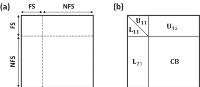
FS F S NF S NFS (a) (b)

Figure 1. A front before (a) and after (b) partial factorization. The fully

summed (FS) variables will be eliminated and the non-fully summed (NFS) variables will be updated. CB is the Schur complement obtained after elim-inating the FS variables.

factorization phase to factorize the system matrix M as M = LDLT

or LU depending on whether M is symmetric or asymmetric; and (3) a solve phase to compute the solution for each RHS via a forward elimination LDy = b to compute an intermediate vector

y, followed by a backward substitution LT_{x = y to compute the}

unknown electric field vector x.

In the multifrontal method, the factorization of M is achieved through a sequence of partial factorizations of relatively small but dense matrices called fronts. As illustrated in Fig. 1, each front is associated with two sets of variables: the fully summed (FS) variables, which are eliminated to get L11 and U11 (by a partial factorization); and the non-fully summed (NFS) variables, which receive updates resulting from the elimination of the FS variables. The fronts are arranged in a tree-shaped graph of dependencies called the ‘elimination tree’ (Schreiber 1982; Liu 1990), which establishes which variables belong to which front and in which order the fronts have to be processed (bottom-up). A fill-reducing ordering such as nested dissection (George1973) can be used to build an efficient elimination tree.

Once a front has been partially factorized, the resulting partial factors L11, L21, U11and U12 are stored in memory, whereas the

Schur complement, the so-called contribution block (CB), is tem-porarily stored in a separate stack. Once it has been used to assemble the parent front later in the factorization process, the CB memory can be freed.

Block Low-Rank matrices

It has been proven that the fronts and CBs resulting from the dis-cretization of elliptic PDEs possess low-rank properties (Bebendorf

2004; Chandrasekaran et al.2010). Even though the matrices them-selves are FR, most of their off-diagonal blocks are usually low-rank. These off-diagonal blocks can be approximated with low-rank rep-resentations, which reduces the flops and memory with a controlled impact on the accuracy of the solution. An efficient method for such an approximation is based on the BLR format studied by Amestoy et al. (2015). It uses a flat block matrix structure which makes it simple and robust as compared to hierarchical matrix formats such as H-matrices (Hackbusch1999), H2_{-matrices (Hackbusch et al.}

2000) and HSS matrices (Xia et al.2010).

Eq. (8) illustrates the BLR representation of a p × p block dense matrix A in which off-diagonal blocks AIJof dimension mI J×nI J

with numerical rank kǫ

AIJ≈YIJZTIJ: A =          A11 A12 A13 · · · A1 p A21 A22 A23 · · · A2 p A31 A32 A33 · · · A3 p .. . ... ... . .. ... Ap1 Ap2 Ap3 · · · App          ≈          A11 Y12Z12T Y13Z13T · · · Y1 pZ1 pT Y21Z21T A22 Y23Z23T · · · Y2 pZ2 pT Y31Z31T Y32Z32T A33 · · · Y3 pZ3 pT .. . ... ... . .. ... Yp1ZTp1 Yp2Zp2T Yp3ZTp3 · · · App          (8)

Here, the matrices YIJand ZIJare of size mI J×kǫI Jand nI J×

kǫ

I J, and the low-rank approximation holds to an accuracy ǫ (the

BLR threshold): ||AIJ−YIJZTIJ|| < ε, where the norm here and

further in the paper is the L2 _{norm. The approximation leads to} savings only when the rank of the block is low enough, typically when kǫ

I J(mI J+nI J) < mI JnI J.

For algebraic operations involving a BLR matrix, the off-diagonal blocks AIJshould be as low-rank as possible to attain the strongest

possible reduction in memory and flops. To understand what deter-mines the rank, we should remind ourselves that every unknown in a matrix obtained from a system of PDEs corresponds to a particular location in the physical space. If the spatial domain occupied by unknowns in block I is far apart from that of unknowns in block J, one can say that the unknowns are weakly connected and the rank of AIJshould be low. Indeed, a very clear correlation between the

geometrical distance between blocks I and J and the rank of the corresponding block matrix has been observed in many studies. In particular, for the case of 3-D seismic problems, this was observed by Weisbecker et al. (2013) and Amestoy et al. (2016). Thus one can use this geometrical principle for optimal clustering of unknowns, the underlying aim being to achieve the best possible low-rank prop-erties for the blocks. Alternatively, if geometrical information is not available, one can use a similar principle based on the matrix graph as shown in Amestoy et al. (2015).

However, the geometrical principle may not work for EM prob-lems as efficient as it does for seismic ones since extreme variations in electrical resistivity over the system lead to vastly different matrix elements. Thus, for two clusters to be weakly connected and have a low rank interaction, it is not sufficient that the corresponding unknowns be located far from each other in space. One should also require that the medium between them not be highly resistive. We will see in the next sections that this nuance may strongly affect the BLR gains for CSEM problems involving the highly resistive air layer. Note that, from a user perspective, it is very desirable that the approach to be able to automatically adapt the amount of low-rank compression to the physical properties of the medium.

Block low-rank multifrontal solver

In order to perform the LU factorization using a BLR multifrontal method, the standard partial factorization algorithm for each front (illustrated in Fig. 1) has to be modified. Several BLR strategies can be considered where the low-rank compression is applied at different stages of operations on the front (Amestoy et al.2015). The strategy used in this work is outlined in Algorithm1. For the sake

Algorithm 1. BLRfactorization of a dense matrix.

Input: a symmetric matrix A of p × p blocks Output: the factors matrices L, D

for k = 1 to p do Factor: LkkDkkLTkk=Akk for i = k + 1 to p do Solve: Lik=AikL−kkTD −1 kk Compress: Lik≈YikZTik for j = k + 1 to i do Update: Aij=Aij −LikDkkLTjk ≈Aij−Yik(ZTikDkkZjk)YTjk end for end for end for

of clarity the algorithm is presented for general dense matrices, but can be easily adapted to the partial factorization of frontal matrices. The frontal matrices are approximated using the BLR format at an accuracy ǫ, and all subsequent operations on them benefit from compression using low-rank products.

The modified multifrontal method derived from Algorithm1has been implemented in the MUMPS solver and is used below to solve systems of equations associated with a number of different matrices arising in CSEM problems. It should be noted that the reduction in the size of the factors provided by the BLR approach has not been exploited yet to reduce the effective memory usage of the solver—implementation of this feature is ongoing. Note that the BLR format can be used to approximate/compress also the CB of the frontal matrix. This could then be used to further reduce the memory footprint of the solver but is out of the scope of this paper. As suggested by theory (Amestoy et al.2017), the block size for the BLR format should depend on the matrix size. The block size was set to 256 on almost all matrices but was increased to 416 for our largest matrix S21. We will refer to the modified multifrontal method as the ‘BLR’ solver, while the MUMPS solver without the BLR feature will be referred to as the FR solver.

R E S U L T S

In this section, we illustrate the efficiency of the BLR solver against the FR solver in terms of factor size, flop count, and run time. This is followed by a comparative study of the performance of the BLR solver in shallow-water and deep-water CSEM modelling scenarios. We then compare the efficiency of both direct solvers against an iterative solver for a realistic CSEM inversion.

In all simulations the system matrix was generated using the finite-difference modelling code presented in Jaysaval et al. (2014). The simulations were carried out on either (1) the CALMIP su-percomputer EOS (https://www.calmip.univ-toulouse.fr/), which is a BULLx DLC system composed of 612 computing nodes, each composed of two Intel Ivybridge processors with 10 cores (total 12 240 cores) running at 2.8 GHz per node and 64 GB/node, or (2) a computer FARAD with 16-core Intel Xeon CPU E5-2690 pro-cessors running at 2.90 GHz and 264 GB memory. The numbers of flops reported corresponds to the number of double precision operations in complex arithmetic.

Models and system matrices

In order to examine the performance of the BLR solver, let us consider the two earth resistivity models depicted in Figs2and3.

10

(km)

5

20

0

15

Figure 2. Vertical cross-section through a simple isotropic 3-D resistivity

model (H-model) at y = 10 km. 0 10 5 15 20 25 30 35 2 4 6 8 0 depth (km) 2 1.5 1 0.5 0 – 0.5

(a)

(b)

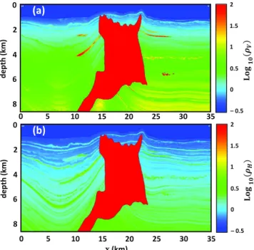
Figure 3. Vertical cross-sections for vertical (a) and horizontal (b)

resistiv-ities of the SEAM model (S-model) at y = 23.7 km.

The model in Fig.2(which we hereafter call the H-model) is a simple isotropic half-space earth model in which a 3-D reservoir of resistivity 100 Ä m and dimension 10 × 10 × 0.2 km3_{is embedded} in a uniform background of resistivity 1 Ä m. It is a shallow-water model: the seawater is 100 m deep and has a resistivity of 0.25 Ä m. The dimensions of the H-model are 20 × 20 × 10 km3_{. A} deep-water variant where the deep-water depth is increased to 3 km (hereafter referred to as the D-model) is also considered and will be described further later. The H and the D models lead to matrices with the same size and structure but different numerical properties.

The model in Fig.3(hereafter the S-model) is the SEAM (SEG Advanced Modeling Program) Phase I salt resistivity model—a complex 3-D earth model designed by the hydrocarbon exploration community and widely used to test 3-D modelling and inversion al-gorithms. The S-model is representative of the geology in the Gulf of Mexico, its dimension is 35 × 40 × 8.6 km3_{, and it includes} an isotropic complex salt body of resistivity 100 Ä m and sev-eral hydrocarbon reservoirs (Stefani et al.2010). The background formation has VTI anisotropy and horizontal ρH and vertical ρV

resistivities varying mostly in the range 0.5–0.6 Ä m. The seawater is isotropic with resistivity 0.3 Ä m, and thickness varying from 625 to 2250 m. However, we chose to remove 400 m from the water column in the original SEAM model, thereby resulting in water depths varying from 225 to 1850 m, to make sure that the air-wave (the signal components propagating from source to receiver via the air) has a significant impact on the data.

The top boundary of both models included an air layer of thick-ness 65 km and resistivity 106 _{Äm. On the five other boundaries} 30 km paddings were added to make sure the combination of strong airwave and zero-field Dirichlet boundary conditions does not lead to edge effects. The current source was an x-oriented horizontal electric dipole (HED) with unit dipole moment at frequency of 0.25 Hz located 30 m above the seabed.

In the padded regions the gridding was severely non-uniform and followed the rules described by Jaysaval et al. (2014), where the air was discretized with 15 cells and the other boundaries with 7 cells. Apart from the padded regions, we used finite-difference grids that were uniform in all three directions. The parameters of five uniform grids used to discretize the H-, D- and S-models are listed in Table1: the cell sizes, number of cells, resulting number of unknowns, and the number of non-zero entries in the system matrix. These discretizations resulted in six different system matrices: H1,

H3/D3 and H17 for the H- and D-models; and S3 and S21 for

the S-model. The numbers represent the approximate number of unknowns, in millions, in the linear systems associated to each matrix; for example, the linear system corresponding to matrix S21 had about 21 million unknowns. So far, for 3-D geophysical EM problems, the largest reported complex-valued linear system that has been solved with a direct solver had 7.8 million unknowns (Puzyrev et al.2016).

Choice of BLR threshold

The BLR threshold ǫ controls the accuracy of the low-rank approx-imation of the dense intermediate matrices in the BLR multifrontal approach. A larger ǫ means larger compression as well as a larger reduction in factor size and flop count, but poorer accuracy of the solution. Therefore, it is necessary to find out which choices of ǫprovide acceptable CSEM solution accuracies, and what are the associated reductions in factor size, flops and run time.

Let us define the relative residual norm δ for matrix eq. (7) as the ratio of residual norm ||s − Mxǫ_{||for an approximate BLR solution}

xǫ_{at BLR threshold ǫ to the zero-solution residual norm ||s|| as}

δ =||s − Mx ǫ_||

||s|| . (9)

The linear systems corresponding to the matrices H1, H3, S3,

H17 and S21 are then solved for different values of ǫ to examine

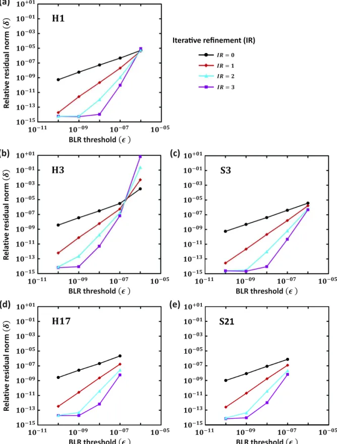
its influence on δ. For all the linear systems, the RHS vector s corresponds to an HED source located 30 m above the seabed in the centre of the model. Fig.4shows the relative residual norm δ plotted as a function of the BLR threshold ǫ. The different curves on each plot correspond to different numbers of iterative refinement steps. Iterative refinement improves the accuracy of the solution of linear systems by the iterative process illustrated in Algorithm2. It has been shown by Arioli et al. (1989) that the accuracy of an approximate solution can be significantly improved with only two to three steps of iterative refinement when the initial approximate solution is reasonable—a result that is also observed for our BLR solutions.

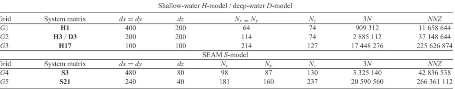
Table 1. Parameters of the uniform grids used to discretize the 3-D shallow-water H-model, deep-water D-model and the SEAM S-model. Here d x, d y, and

d z are the cell sizes in meters, while Nx, Nyand Nzare the number of cells in x-, y-, and z-directions that also include non-uniform cells added to pad the

model at the edges. 3N = 3Nx×Ny×Nzis the total number of unknowns and N N Z is the total number of non-zero entries in the system matrix.

Shallow-water H-model / deep-water D-model

Grid System matrix dx = dy dz Nx =Ny Nz 3N NNZ

G1 H1 400 200 64 74 909 312 11 658 644

G2 H3 / D3 200 200 114 74 2 885 112 37 148 644

G3 H17 100 100 214 127 17 448 276 225 626 874

SEAM S-model

Grid System matrix dx = dy dz Nx Ny Nz 3N NNZ

G4 S3 480 80 98 87 130 3 325 140 42 836 538

G5 S21 240 40 181 160 237 20 590 560 266 361 112

A conventional choice for the convergence criterion for itera-tive solvers used for EM problems, see for example, Newman & Alumbaugh (1995), Smith (1996) and Mulder (2006) is δ ≤ 10−6_. Fig.4shows that the BLR threshold ǫ should be ≤ 10−7_{to fulfill} this criterion for all the linear systems. Iterative refinement reduces the relative residual norm δ, but it comes at the cost of an additional forward-backward substitution per refinement step (step 3 of Algo-rithm2) at the solution stage. For the case of thousands of RHSs, which is typical for a CSEM inversion problem, these iterative steps may be too costly. Therefore, the focus of the following discussions is on the BLR solution obtained without any iterative refinement. It follows from Fig.4that the corresponding curves δ(ǫ) look quite similar for all the matrices included in the study. This is a good sign that gives reason to hope that choosing ǫ < 10−7 _{will guarantee} good accuracy of the solution for most practical CSEM problems. Furthermore, the fact that the accuracy in the solution smoothly decreases when ǫ increases, also adds confidence in the robustness and usability of the BLR method in a production context.

Let us now investigate the accuracy of the BLR solution xǫ_for different values of ǫ and analyze the spatial distribution of the solution error. The error is defined as the relative difference between the BLR solutions xǫ_{and the FR solution x :}

ξm,i, j,k= v u u u t ¯ ¯xǫ_{m,i, j,k}−xm,i, j,k ¯ ¯ 2 ³_¯ ¯xǫ_{m,i, j,k} ¯ ¯ 2 +¯¯xm,i, j,k ¯ ¯ 2´ /2 + η2 , (10) for m = x, y and z; i = 1, 2, . . . Nx; j = 1, 2, . . . Ny; k =

1, 2, . . . Nz. Here, xm,i, j,krepresents the m-component of the electric

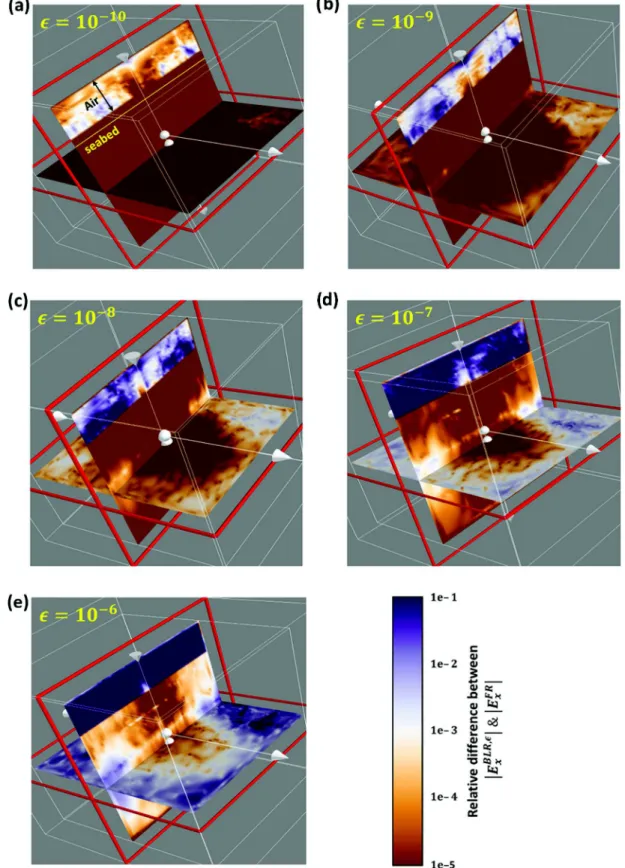
field at the (i, j, k)th node of the grid, while η = 10−16 _{V m}−1 represents the ambient noise level. Fig.5shows 3-D maps of the relative difference ξx,i, j,kbetween xǫand x for the x-component of

the electric field for matrix H3.

In all maps the relative error in the air is orders of magnitude larger than in the water or formation. Similar observations have been earlier reported by Grayver & Streich (2012). Fortunately, large errors in the air do not create a problem in most practical CSEM applications. For marine CSEM inversion one needs very high accuracy for the computation of the EM fields at the seabed receivers—to compare them to the measured data, as well as rea-sonably accurate fields in the whole inversion domain—to compute the corresponding Jacobians and/or gradients. However, one never inverts for the air resistivity, hence we can exclude the air from the analysis and focus on the solution errors only in the water and the earth.

One can see from Fig. 5that for the smallest BLR threshold, ǫ =10−10 _{, the relative error ξ}

x,i, j,k in water and formation is

negligible (∼10−4_{), but it increases for larger ǫ, and for ǫ = 10}−8 and 10−7_{reaches 1–2 per cent at depth, though remains negligible}

close to the seabed and at shallow depths. For ǫ = 10−6 _{the error} exceeds 10 per cent in the deeper part of the model, implying that the BLR solution xǫ _{obtained with ǫ = 10}−6 _{is of poor quality.} At the same time, solutions obtained with ǫ ≤ 10−7 _{are accurate} enough and can be considered appropriate for CSEM modelling and inversion. We also computed the error ξz,i, j,kfor the z-component

of the electric field and found very similar behavior as in Fig.5.

Performance of BLR solver

Let us now examine how the factorization flop count and memory requirements for storing the LU factors are reduced in the BLR solver compared to the FR solver. A clear reduction is demonstrated in Fig.6, showing results for five matrices H1, H3, S3, H17 and

S21, for different values of the BLR threshold ǫ. The benefits of

the BLR solver are quite significant: the factor storage can go down to 30 per cent of its FR value, while flops can go even below 10 per cent. Note also that both factor storage and flops only gently decrease as ǫ increases from 10−10_{to 10}−7_{. This is quite an important} property of the BLR solver; first because finding the optimal value of the threshold is thus not a critical issue, and second because it allows for significant computational savings even in the presence of stringent requirements on the solution accuracy.

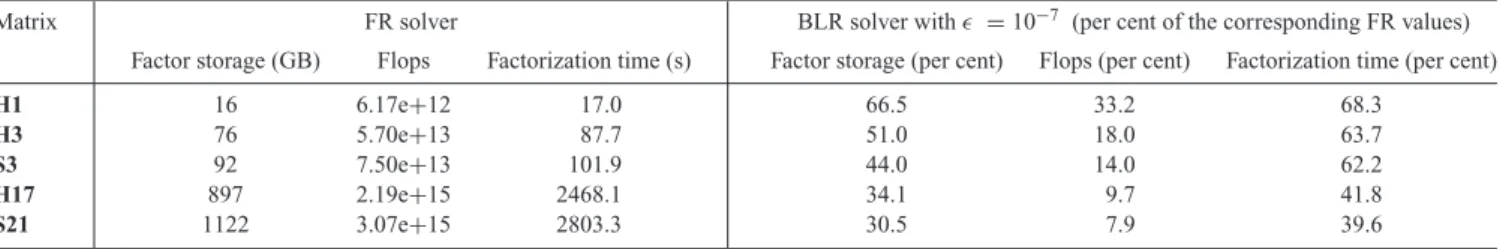
Fig.7illustrates how the observed reduction in flops propagates into reduction in the elapsed run time for a specific example on the EOS supercomputer using 90 MPI processes with 10 threads, that is, a total of 900 cores. The time reduction being evaluated with respect to the FR factorization time, it is important to mention that on matrix S21 the FR solver reaches 22 per cent of the peak per-formance of the 900 cores, which is quite a good perper-formance for a sparse direct solver. All factorizations here assume the BLR thresh-old is set to ǫ = 10−7_{, which provides a good solution accuracy} as shown in the previous section. We chose a hybrid paralleliza-tion setting: 1 MPI-task per node and 10 threads per MPI-task in order to meet the memory requirements for the factorization of the largest matrices H17 and S21 while at the same time allowing for an efficient use of multithreaded BLAS routines within MUMPS. Table2shows the factor storage, flops, and elapsed run times for the factorization of all matrices using both the FR and BLR solvers. For the FR solver these metrics are given as absolute numbers, while for the BLR solver they are normalized to the corresponding FR metrics. The normalized BLR metrics are also plotted in Fig.7. Compared to Fig.6, low-rank results in Fig.7and Table2are ob-tained with a setting that applies slightly less compression when this can boost performance, sometimes leading to slightly larger values for the flop count and factor size (e.g. on H1). Still, it is easy to see that the observed reduction in run time is weaker than the reduction in flops; for example, for the biggest S21 matrix the

(a)

mr

o

n l

a

u

di

s

er

e

vi

t

al

e

R

BLR threshold

IteraGve refinement (IR)

(c)

mr

o

n l

a

u

di

s

er

e

vi

t

al

e

R

BLR threshold

BLR threshold

(b)

mr

o

n l

a

u

di

s

er

e

vi

t

al

e

R

BLR threshold

BLR threshold

21

(e)

(d)

Figure 4. Plots of the relative residual norm δ as a function of the BLR threshold ǫ for linear systems corresponding to matrices H1, H3, S3, H17 and S21.

The residual δ is always below 10−6_{if one chooses ǫ ≤ 10}−7_.

BLR flops are 8 per cent of their FR value, whereas the run time amounts to only 40 per cent of the FR value. This is a result of the relatively lower efficiency of the low-rank kernels due to the smaller granularities involved in the BLR factorization; and also

a result of the fact that the relative weight of the overhead corre-sponding to non-floating-point operations (such as MPI communi-cation, assembly operations and data access) is higher in the BLR case.

Algorithm 2. Iterative refinement step(s).

1. Compute the residual: r = s − Mxǫ_{for the BLR solution x}ǫ

2. repeat

3. Solve M1x = r using the LU or LDLT_{factors of M}

4. xǫ_←xǫ_{+ 1x}

5. r = s − Mxǫ

6. compute δ = |s − Mxǫ_|/|s|

7. until δ is below a tolerance level or maximum number of iterations is reached

It is known that low-rank approximations become more efficient as matrix sizes grow. As a result, the gains due to BLR approxi-mations are larger for bigger matrices, which is in agreement with the present study as can be seen from Fig.7for all the plotted met-rics: flops, storage and run time. Earlier studies on 3-D Laplacians (Amestoy et al. 2015) experimentally showed that the MUMPS-BLR solver has O(N1.65_{) complexity in the number of flops, a} significant improvement from the standard O(N2_{) complexity for} FR factorization, while the experimental complexity for 3-D seis-mic problems was found to be in O(N1.78_{). All these results are} quite close to the theoretical prediction for complexity of the BLR factorization, O(N1.7_{), recently computed by Amestoy et al. (2017).} We also performed a power regression analysis of the flops data in Table2: they show the expected N2 _{trend for the FR data, while} for BLR the dependence was Nm _{with m =1.6 ± 0.1. Thus, the}

observed reduction in flops complexity for the 3-D CSEM problem is consistent with theoretical results and is close to those reported for 3-D Helmholtz equations. In the next section we discuss how the flop count is affected by removing the air layer, which strongly reduces the scale of resistivity variations in the model.

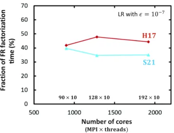
It is also important to study how the gain due to the BLR approx-imation evolves with the number of cores. Fig.8shows ratio of the BLR factorization time over the FR factorization time. This ratio is presented for different numbers of MPI processes and/or numbers of threads for the system matrices H17 and S21. Ideally, this ratio should remain constant when the number of cores increases. This is more or less the case, as only small variations can be observed. Thus, Fig.8illustrates the ability of the BLR solver to maintain an important gain with respect to the FR solver, even on higher numbers of cores. The corresponding factorization times are listed in Table3(where data or matrix H1 is also included).

Deep water versus shallow water

The benefits of the BLR solver depend on how efficiently blocks of frontal matrices can be compressed using low-rank approximations. As discussed above, compression of a block matrix AIJis expected

to be efficient when the spatial domains corresponding to unknowns

I_{and J are far from each other and the two sets of unknowns are}

thus weakly connected. This has been demonstrated for 3-D seismic problems by directly plotting the rank of AIJ versus the distance

between domains I and J (Amestoy et al. 2015). One complica-tion for CSEM problems is the presence of the insulating air layer whose resistivity is typically many orders of magnitude higher than that in the rest of the computational domain. EM signals propagate through the air almost instantaneously, as compared to relatively slow propagation through conductive water or sediments. There-fore, two regions located close to the air are effectively connected to each other via the so called air-wave even if these regions are geometrically very far apart. It is interesting to know whether this interconnectivity via the air layer can degrade the low-rank proper-ties of corresponding matrices and affect performance of the BLR

solver. Therefore, in this section we present additional simulations for earth models that do not include an air layer.

The results presented in the previous sections are based on a shallow-water H-model (water depth of 100 m) and the S-model with water depth varying from 225 to 1850 m. In both cases, the airwave strongly affects the subsurface response at most source-receiver offsets at the chosen frequency of 0.25 Hz (Andreis & MacGregor

2008). On the other hand, if the water depth is increased to 3 km, the airwave contribution becomes negligible because EM fields are strongly attenuated in the conductive sea water (see e.g. Jaysaval et al.2015). Keeping this in mind, we built a deep-water model (D-model) from the shallow-water H-model by simply removing the air layer and adding 2.9 km of seawater so that the water layer becomes 3 km thick. The source is again an x-oriented HED with a frequency of 0.25 Hz placed 30 m above the seabed. The D-model was discretized using the same grid (Table1) as the H-model, which resulted in matrix D3 having the same dimensions and number of nonzero entries as H3. The results of simulations performed on the FARAD computer using 2 MPIs × 8 threads = 16 cores and BLR threshold ǫ = 10−7 _{are presented in Table4.}

The FR numbers are essentially identical for the shallow-water and deep-water matrices, which is somewhat expected as the ma-trices have the same number of unknowns and the same structure. On the other hand, it once again demonstrates the robustness of the direct solver whose efficiency is not affected by replacing the conductive water layer with extremely resistive air which changes values of the corresponding matrix elements by —six to seven or-ders of magnitude. In contrast, many iterative solvers struggle to converge in the presence of an air layer because it makes the system matrix more ill-conditioned due to high resistivities and large aspect ratios of some cells (see e.g. Mulder2006).

Most importantly, the gains achieved by using the BLR function-ality are larger for the deep-water matrix D3 than for the shallow-water matrix H3. This is especially evident for the factorization flops that amount to only 12.0 per cent of the FR flops for D3, while for the H3 matrix that number increases to 16.3 per cent. It is inter-esting to investigate how the observed difference in flops between the deep and shallow-water matrices depends on the matrix size. For that purpose we generated 11 additional grids for discretization of the H- and D-models. We started with a grid resulting in 4.9 million unknowns, which was constructed along the same lines as the other grids in Table1, but with dx = dy = dz = 167 m. The next grid was obtained by making all its cells proportionally coarser by 5–10 per cent, and so on for next grids. The rate at which the cell sizes were increasing, was identical in all parts of the model (air, water, formation, reservoir, non-uniform paddings) and all direc-tions: x, y and z. The number of unknowns for the smallest grid was ∼516 000.

Fig.9shows how the factorization flops depend on the number N of unknowns for this set of grids. The FR solver has the expected O(N2_{) complexity for both types of matrices. The BLR} compres-sion significantly reduces complexity, but the reduction depends on

Figure 5. Relative difference between the BLR solution xǫ_{for different BLR thresholds ǫ, and the FR solution x for a linear system corresponding to matrix} H3. For ǫ = 10−7_{, the solution accuracy is acceptable everywhere except in the air layer at the top. The results are for the x-component of the electric field.}

The air and PML layers are not to scale.

the matrix type. For matrices obtained from shallow-water model H, we observe an O(Nm_{) behavior with m = 1.58 ± 0.02. This is}

in a very good agreement with the value m = 1.6 ± 0.1 found in the previous section for models H and S (both can be considered

to be shallow-water models), but a different set of grids. At the same time, Fig.9shows that for deep-water model D complexity is reduced even further, down to m = 1.40 ± 0.01. This confirms that the BLR savings are consistently larger for deep-water matrices

n

oi

t

az

ir

ot

c

af

R

F f

o

n

oi

tc

ar

F

flops

(%)

BLR threshold

(b)

BLR threshold

(a)

e

g

ar

ot

s

r

ot

c

af

R

F f

o

n

oi

tc

ar

F

(%)

Figure 6. Fraction of FR factor storage (a) and flops (b) required by

the BLR solver to factorize H1, H3, S3, H17 and S21 for different BLR thresholds ǫ.

and also shows that this effect becomes stronger for larger systems. For example, for the system with 4.9 million unknowns, the factor-ization of the shallow-water matrix requires 71 per cent more flops than factorization of the deep-water matrix.

Fig.10shows data for the factor storage computed for the same set of 11 grids with different number of unknowns. One can see that the BLR method also reduces the factor storage complexity. Namely, the FR behaviour of O(Nm_{) with m = 1.38 ± 0.01 is}

changed to m = 1.18 ± 0.01 for a shallow water case, while for a deep-water case the BLR reductions are even stronger: down to m = 1.14 ± 0.01. These values are very close to the FR and BLR exponents, 1.36 and 1.19, reported for a 3-D seismic problem, and in agreement with the theoretical FR and BLR predictions, 1.33 and 1.17, respectively (Amestoy et al.2017).

0 10 20 30 40 50 60 70 80 Matrices Fr acGon of FR (%) _{factorizaGon Gme} factor storage factorizaGon flops LR with = 10

Figure 7. Fraction of the FR factor storage, flops and elapsed time (on 90

×10 cores of EOS) required by the BLR solver with ǫ = 10−7 _{to factorize} H1, H3, S3, H17 and S21.

Deep water model D is different from model H in two ways: it has a thicker water layer and does not contain air. We made an additional test run for a model with both a thick water layer and an air layer, and found the results to be similar to those for the H-model. It allows us to conclude that the observed improvements in the performance of BLR solver for the deep-water matrices are mainly due to removal of the highly resistive air layer. Presence of the air layer effectively interconnects model domains located close to the air interface, as discussed above. It should lead to higher rank of the corresponding block matrices and make low-rank approximations less efficient. In other words, the air introduces non-locality into the system: in some numerical schemes the air is simply excluded from the computational domain and replaced by a non-local boundary condition at the air-water interface (Wang & Hohmann1993). Thus, one may argue that the air effectively increases dimensionality of the system, which in turn, should also increase complexity.

Suitability of BLR solvers for inversion

Direct solvers are very well suited for multisource simulations since once the system matrix M is factorized, the solution for each RHS can be computed using relatively inexpensive forward-backward substitutions. Therefore, they are particularly attractive for applica-tions involving large-scale CSEM inversions where the number of RHSs can reach several thousands. Nevertheless, the computational cost of the factorization phase remains huge and often dominates, tipping the balance in favour of simpler iterative solvers. For ex-ample, even for relatively small CSEM matrices with ∼3 million unknowns, an iterative solver is shown to be superior as long as Table 2. Factor storage, flops and elapsed run times needed for factorization of all H and S matrices using FR and BLR solvers. Values for the BLR solver are

given as a percentage of the corresponding FR values. Savings due to the BLR method are significant and grow with increasing matrix size. The factorizations are carried out on EOS supercomputer using a 90 MPI tasks × 10 threads setting.

Matrix FR solver BLR solver with ǫ = 10−7 _{(per cent of the corresponding FR values)}

Factor storage (GB) Flops Factorization time (s) Factor storage (per cent) Flops (per cent) Factorization time (per cent)

H1 16 6.17e+12 17.0 66.5 33.2 68.3

H3 76 5.70e+13 87.7 51.0 18.0 63.7

S3 92 7.50e+13 101.9 44.0 14.0 62.2

H17 897 2.19e+15 2468.1 34.1 9.7 41.8

n

oi

t

az

ir

ot

c

af

R

F f

o

n

oi

tc

ar

F

Gme

(%)

Number of cores

Figure 8. Fraction of the FR factorization time required by BLR

factor-ization for different numbers of MPI tasks and threads. The ratio between BLR and FR times does not vary significantly when the number of cores increases, illustrating the ability of the BLR solver to maintain important gains even on higher numbers of cores.

the number of RHSs is kept below 150 (Grayver & Streich2012). In this section we benchmark our direct solver with and without BLR functionality against an iterative solver for an application in a realistic CSEM inversion based on the SEAM model.

Let us consider inversion of synthetic CSEM data over the S-model of Fig.3. We assume that nr =121 receivers are used to

record simulated responses. For each receiver, HED sources are located along 22 towlines (11 in the x- and 11 in the y-directions) with an interline spacing of 1 km. Each towline has a length of 30 km with independent source positions 200 m apart. This implies 150 source positions per towline, or a total of ns = 22 × 150 = 3300

source positions. The model is discretized with grid G5 defined in Table1, which results in system matrix S21 with 20.6 million unknowns. The frequency is 0.25 Hz.

To invert the CSEM responses with the above acquisition param-eters, we consider two inversion schemes: (1) a quasi-Newton inver-sion scheme described in Zach et al. (2008); and (2) a Gauss-Newton inversion scheme described in Amaya (2015). An inversion based on

5 6 6

.

.

Figure 9. Factorization flop count for shallow-water and deep-water

matri-ces with different number of unknowns. The full-rank complexity O(N2_{) is}

independent of the water-depth. The low-rank method reduces complexity for shallow-water matrices to O(Nm_{), with m = 1.58. The improvement is}

even stronger in deep water, where m = 1.40, indicating better BLR com-pression rates in the absence of resistive air.

5 6 6

.

.

Figure 10. Factor storage for shallow-water and deep-water matrices with

different number of unknowns N . The memory needed to store factors grows as a power law, O(Nm_{), and the use of the BLR solver significantly reduces}

the value of exponent m. The reduction is slightly stronger for the deep water case.

the Gauss–Newton scheme converges faster and is less dependent on the starting model as compared to the quasi-Newton inversion, but this comes at the cost of increased computational complexity. We refer to Habashy & Abubakar (2004) for a detailed discussion of Table 3. Factorization times (s) for H1, H17 and S21 matrices by the FR and BLR (with ǫ = 10−7_{) solvers for different parallelization}

settings (MPI tasks × threads of EOS supercomputer).

Matrix Solver Factorization time (s) using MPI × threads =

64 × 1 64 × 4 64 × 10 90 × 10 128 × 10 192 × 10 H1 FR 53.8 23.1 18.8 BLR 36.7 19.4 14.8 H17 FR 2468.2 1848.0 1329.5 BLR 1033.1 885.0 589.7 S21 FR 2803.3 2536.6 2196.1 BLR 1112.9 878.4 768.4

Table 4. Factor storage, flops and elapsed run times needed for factorization of shallow-water (H3) and deep-water (D3) matrices. Values for the BLR solver

are given as a percentage of the corresponding FR values. The factorizations are performed on 16 cores of FARAD computer.

Matrix, water depth FR solver BLR solver with ǫ = 10−7_{(per cent of the corresponding FR values)}

Factor storage (GB) Flops Factorization time (s) Factor storage (per cent) Flops (per cent) Factorization time (per cent)

H3, shallow 76 5.7 × 1013 _{986 49.5 16.3 32.8}

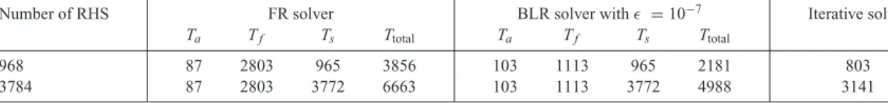
Table 5. Run times (s) for the FR and BLR direct solvers on EOS computer as well as for a multigrid preconditioned iterative solver

to perform CSEM simulations for a large number of RHSs. The first row with 968 RHSs corresponds to an inversion iteration using a quasi-Newton scheme applied to CSEM data over the SEAM model, while the second row with 3784 RHSs to the Gauss–Newton inversion scheme. The simulations are carried out for the system matrix S21 using 900 computational cores. For the direct solvers, Ta

is the analysis time, Tf is the factorization time, Tsis the solve time (for forward-backward substitutions for all RHSs) and Ttotalis the

total time, all measured in seconds.

Number of RHS FR solver BLR solver with ǫ = 10−7 _{Iterative solver}

Ta Tf Ts Ttotal Ta Tf Ts Ttotal

968 87 2803 965 3856 103 1113 965 2181 803

3784 87 2803 3772 6663 103 1113 3772 4988 3141

the theoretical differences between the two inversion schemes. One key difference is the number of RHSs that needs to be handled at each inversion iteration. For the quasi-Newton scheme it scales with the number of receivers nr, while in the Gauss–Newton scheme one

should include computations also for all source shot points ns.In a

typical marine CSEM survey one has ns ≫nr, hence the number

of RHSs required by the Gauss–Newton scheme is much larger than that by the quasi-Newton scheme.

Let us start with the quasi-Newton inversion scheme. For the chosen example based on the SEAM model, it requires 968 RHSs (4 [field components Ex, Ey, Hx, and Hy] × 2 [direct and adjoint

modelling] × 121 [nr]) per inversion iteration for one frequency.

The first row of Table5shows the analysis, factorization, forward-backward substitutions for all RHSs, and total solution times using FR and BLR solvers on the EOS supercomputer using 90 MPI × 10 threads setting and ParMetis (Karypis & Kumar1998) for order-ing. For comparison, time estimates for an iterative solver are also presented in Table5. This iterative solver was developed following the ideas of Mulder(2006): a complex biconjugate-gradient-type solver, BICGStab(2) (van der Vorst1992; Gutknecht1993) is used in combination with a multigrid pre-conditioner and a block Gauss– Seidel type smoother. Here the run time was evaluated assuming that there are 968 modelling jobs (one job per RHS), with each job running on a dedicated core and the total number of cores the same as for the direct solver, that is, 900. The run time for a specific iterative solver job was estimated by sending the same job to all cores at once and taking the average run time. We also took into account the fact that a modelling job for a given RHS is limited to the section of the SEAM model which is effectively illuminated by a given source. The lateral dimensions of this sub-model were chosen as 28 × 28 km2_{. Though the BLR solver is almost twice as} fast as the FR direct solver, it is still —two to three times slower than the iterative solver for 968 RHSs (first row of Table5).

Let us now look at the second row of Table5showing results for the Gauss–Newton inversion scheme. Even though the number of rows in Jacobian scales as nsnr(per frequency), all its elements can

be computed by solving the forward problem only for ns+4nr

right-hand sides, see for example, appendix in Amaya (2015). Thus we arrive at 3300 + 484 = 3784 RHSs per inversion iteration per fre-quency. The total time for the BLR solver, 4988 s, is still larger than 3141 s for the iterative solver implying that with the current implementation of both solvers the iterative solver is a better choice for the modelling engine of a 3-D CSEM inversion. However, the time spent on matrix factorization with the BLR solver, 1113 s, is now much smaller than the iterative solver time. It is actually the solve phase, where forward-backward substitutions for each RHS are performed, that remains relatively slow (approximately 1 second per 1 RHS) and makes the direct solver less competi-tive. Here we should emphasize that the current implementation of

the BLR solver does not exploit the BLR compression of factors in the solve phase. Hence computational complexity remains the same for the FR and BLR solvers; one can easily see from Table5

that the solve phase times for both solvers are identical. There is a clear potential to speed up the forward-backward substitutions by using the BLR compressed factors computed at the factorization phase, and in addition by working on the parallelism and perfor-mance of the solve phase. This is planned future work. For this example, if the BLR gains at the solve phase turn out to be com-parable to those of the factorization phase, the BLR solver would become more attractive than the iterative solver for 2500 or more RHSs.

C O N C L U S I O N S

We have demonstrated that application of BLR multifrontal func-tionality to solve linear systems arising in finite-difference 3-D EM problems leads to significant reductions in matrix factor size, flop count and run time as compared to a FR solver (without BLR func-tionality). The savings increase with the number of unknowns N; for example, for the factorization flop count, the O(N2_{) scaling for} the FR solver is reduced to O(Nm_{) with m = 1.4—1.6 for the}

BLR solver. This is slightly better than the theoretical complexity computed by Amestoy et al. (2017). Matrices with up to 20 million unknowns have been factored showing the BLR flops going down to 10 per cent, and the factorization time down to 40 per cent of the FR values. For shallow-water EM problems, we have shown that the reduction due to BLR approach is less than for deep water. This may be related to the highly resistive air layer that increases connectivity between system unknowns and hence decreases low-rank compres-sion rates. The BLR solver runtimes were compared to those of an iterative solver with multigrid preconditioning in an inversion sce-nario where simulations at multiple source locations are necessary. For a few thousand RHSs, which is typical in Gauss-Newton CSEM inversion schemes today, the BLR solver delivers comparable run times and could potentially outperform the iterative solver once BLR functionality is used not only for matrix factorization, but also for forward-backward substitutions.

A C K N O W L E D G E M E N T S

We thank EMGS for giving permission to publish the results. We are also grateful to our collaborators from the MUMPS team A. Guermouche, G. Joslin and C. Puglisi as well as to T. Støren from EMGS. This work was granted access to the HPC resources of CALMIP under the allocation 2015–P0989.

R E F E R E N C E S

Amaya, M., 2015. High order optimization methods for large-scale 3D CSEM data inversion, PhD thesis, Norwegian University of Science and Technology, Trondheim. Available at: http://hdl.handle. net/11250/2365341, 27 March 2017.

Amestoy, P.R., Duff, I.S., L’Excellent, J.-Y. & Koster, J., 2001. A fully asynchronous multifrontal solver using distributed dynamic scheduling, SIAM J. Matrix Anal. Appl., 23, 15–41.

Amestoy, P.R., Guermouche, A., L’Excellent, J.-Y. & Pralet, S., 2006. Hybrid scheduling for the parallel solution of linear systems, Parallel Comput.,

32, 136–156.

Amestoy, P.R., Ashcraft, C., Boiteau, O., Buttari, A., L’Excellent, J.-Y. & Weisbecker, C., 2015. Improving multifrontal methods by means of block low-rank representations, SIAM J. Sci. Comput., 37(3), A1451–A1474. Amestoy, P.R., Brossier, R., Buttari, A., L’Excellent, J.-Y., Mary, T.,

M´etivier, L., Miniussi, A. & Operto, S., 2016. Fast 3D frequency-domain full waveform inversion with a parallel Block Low-Rank multifrontal di-rect solver: application to OBC data from the North Sea, Geophysics,

81(6), 363–83.

Amestoy, P.R., Buttari, A., L’Excellent, J.-Y. & Mary, T., 2017. On the complexity of the Block Low-Rank multifrontal factorization, accepted for publication in SIAM J. Sci. Comput.

Andreis, D. & MacGregor, L., 2008. Controlled-source electromagnetic sounding in shallow water: principles and applications, Geophysics, 73, F21–F32.

Arioli, M., Demmel, J. & Duff, I.S., 1989. Solving sparse linear sys-tems with sparse backward error, SIAM J. Matrix Anal. Appl., 10(2), 165–190.

Avdeev, D.B., 2005. Three-dimensional electromagnetic modelling and in-version from theory to application: Surv. Geophys., 26, 767–799. Bebendorf, M., 2004. Efficient inversion of the Galerkin matrix of

gen-eral second-order elliptic operators with nonsmooth coefficients, Math. Comput., 251, 1179–1199.

Blome, M., Maurer, H.R. & Schmidt, K., 2009. Advances in three-dimensional geoelectric forward solver techniques, Geophys. J. Int.,

176(3), 740–752.

B¨orner, R.U., 2010. Numerical modeling in geo-electromagnetics: advances and challenges, Surv. Geophys., 31, 225–245.

Chandrasekaran, S., Dewilde, P., Gu, M. & Somasunderam, N., 2010. On the numerical rank of the off-diagonal blocks of Schur complements of discretized elliptic PDEs, SIAM J. Matrix Anal. Appl., 31, 2261–2290. Constable, S., 2010. Ten years of marine CSEM for hydrocarbon exploration,

Geophysics, 75(5), A67–A81.

da Silva, N.V., Morgan, J.V., Macgregor, L. & Warner, M., 2012. A finite element multifrontal method for 3D CSEM modeling in the frequency-domain, Geophysics, 77(2), E101–E115.

Davis, T.A., 2004. Algorithm 832: UMFPACK V4.3—an unsymmetric-pattern multifrontal method, ACM Trans. Math. Softw., 30, 196–199. Davydycheva, S., 2010. 3D modeling of new-generation (1999–2010)

resis-tivity logging tools, Leading Edge, 29(7), 780–789.

Duff, I., Erisman, A. & Reid, J., 1986. Direct Methods for Sparse Matrices, Oxford University Press.

Ellingsrud, S., Eidesmo, T., Sinha, M.C., MacGregor, L.M. & Constable, S., 2002. Remote sensing of hydrocarbon layers by seabed logging (SBL): results from a cruise offshore Angola, Leading Edge, 21, 972–982.

George, A., 1973. Nested dissection of a regular finite element mesh, SIAM J. Numer. Anal., 10, 345–63.

Grayver, A. & Streich, R. 2012. Comparison of iterative and direct solvers for 3D CSEM modeling, SEG Extended Abstracts, pp. 1–6, doi:10.1190/segam2012-0727.1.

Gupta, A. & Avron, H., 2000. WSMP: Watson Sparse Matrix Pack-age Part I – Direct Solution of Symmetric Systems, Available at:

http://researcher.watson.ibm.com/researcher/files/us-anshul/wsmp1.pdf, last accessed 27 March 2017.

Gutknecht, M.H., 1993. Variants of BiCGStab for matrices with complex spectrum, SIAM J. Sci. Stat. Comput., 14(5), 1020–1033.

Habashy, T.M. & Abubakar, A., 2004. A general framework for constraint minimization for the inversion of electromagnetic measurements, Inverse Probl., 46, 265–312.

Hackbusch, W., 1999. A sparse matrix arithmetic based on H-matrices. Part I: Introduction to H-matrices, Computing, 62, 89–108.

Hackbusch, W., Khoromskij, B. & Sauter, S.A., 2000. On H2-matrices, in Lectures on Applied Mathematics: Proceedings of the Sympo-sium Organized by the Sonderforschungsbereich 438 on the Occa-sion of Karl-Heinz Hoffmann’s 60th birthday, Munich, June 30 – July 1, 1999, eds Bungartz, H.-J., Hoppe, R.H.W. & Zenger, C., Springer.

Jaysaval, P., Shantsev, D. & de la Kethulle de Ryhove, S., 2014. Fast multimodel finite-difference controlled-source electromagnetic simu-lations based on a Schur complement approach, Geophysics, 79(6), E315–E327.

Jaysaval, P., Shantsev, D.V. & de la Kethulle de Ryhove, S., 2015. Efficient 3-D controlled-source electromagnetic modelling us-ing an exponential finite-difference method, Geophys. J. Int., 203(3), 1541–1574.

Jaysaval, P., Shantsev, D.V, de la Kethulle de Ryhove, S. & Bratteland, T., 2016. Fully anisotropic 3-D EM modelling on a Lebedev grid with a multigrid preconditioner and its application to inversion, Geophys. J. Int.,

207, 1554–1572.

Karypis, G. & Kumar, V., 1998. A parallel algorithm for multilevel graph partitioning and sparse matrix ordering, J. Parallel Distrib. Comput., 48, 71–95.

Key, K., 2012. Marine electromagnetic studies of seafloor resources and tectonics, Surv. Geophys., 33, 135–167.

Li, X.S. & Demmel, J.W., 2003. SuperLU DIST: A scalable distributed-memory sparse direct solver for unsymmetric linear systems, ACM Trans. Math. Softw., 29, 110–140.

Liu, J., 1992. The multifrontal method for sparse matrix solution: Theory and practice, SIAM Rev., 34, 82–109.

Liu, J.W.H., 1990. The role of elimination trees in sparse factorization, SIAM J. Matrix Anal. Appl., 11, 134–172.

Mulder, W.A., 2006. A multigrid solver for 3D electromagnetic diffusion, Geophys. Prospect., 54, 633–649.

Newman, G.A. & Alumbaugh, D.L., 1995. Frequency-domain modeling of airborne electromagnetic responses using staggered finite differences, Geophys. Prospect., 43, 1021–1042.

Oldenburg, D.W., Haber, E. & Shekhtman, R., 2013. Three dimensional inversion of multisource time domain electromagnetic data, Geophysics,

78(1), E47–E57.

Puzyrev, V., Koldan, J., de la Puente, J., Houzeaux, G., V´azquez, M. & Cela, J.M., 2013. A parallel finite-element method for three-dimensional controlled-source electromagnetic forward modelling, Geophys. J. Int.,

193(2), 678–693.

Puzyrev, V., Koric, S. & Wilkin, S., 2016. Evaluation of parallel direct sparse linear solvers in electromagnetic geophysical problems, Comput. Geosci.,

89, 79–87.

Schenk, O. & G¨artner, K., 2004. Solving unsymmetric sparse systems of linear equations with PARDISO, Future Gener. Comput. Syst., 20, 475– 487.

Schreiber, R., 1982. A new implementation of sparse Gaussian elimination, ACM Trans. Math. Softw., 8, 256–276.

Smith, J.T., 1996. Conservative modeling of 3-D electromagnetic fields, Part II: Biconjugate gradient solution and an accelerator, Geophysics, 61, 1319–1324.

Stefani, J., Frenkel, M., Bundalo, N., Day, R. & Fehler, M., 2010. SEAM update: Models for EM and gravity simulations, Leading Edge, 29, 132– 135.

Streich, R., 2009. 3D finite-difference frequency-domain modeling of controlled-source electromagnetic data: direct solution and optimization for high accuracy, Geophysics, 74(5), F95–F105.

van der Vorst, H.A., 1992. BI-CGSTAB: a fast and smoothly converging variant of bi-CG for the solution of nonsymmetric linear systems, SIAM J. Sci. Stat. Comput., 13(2), 631–644.

Wang, T. & Hohmann, G.W., 1993. A finite-difference, time-domain solu-tion for three dimensional electromagnetic modeling, Geophysics, 58(6), 797–809.

Wang, S., de Hoop, M.V. & Xia, J., 2011. On 3D modeling of seismic wave propagation via a structured parallel multifrontal direct Helmholtz solver, Geophys. Prospect., 59, 857–873.

Weisbecker, C., Amestoy, P., Boiteau, O., Brossier, R., But-tari, A., L’Excellent, J.Y., Operto, S. & Virieux, J., 2013. 3D frequency-domain seismic modeling with a block low-rank algebraic multifrontal direct solver, SEG Extended Abstracts, pp. 3411–3416.

Xia, J., Chandrasekaran, S., Gu, M. & Li, X.S., 2010. Fast algorithms for hierarchically semiseparable matrices, Numer. Linear Algebr. Appl., 17, 953–976.

Yee, K., 1966. Numerical solution of initial boundary value problems in-volving Maxwell’s equations in isotropic media, IEEE Trans. Antennas Propag., 14, 302–307.

Zach, J.J., Bjørke, A.K., Støren, T. & Maaø, F., 2008. 3D inversion of marine CSEM data using a fast finite-difference time-domain for-ward code and approximate Hessian-based optimization, in Proceedings of the 78th Annual International Meeting, SEG, Expanded Abstracts, pp. 614–618.