O
pen
A
rchive
T
OULOUSE
A
rchive
O
uverte (
OATAO
)
OATAO is an open access repository that collects the work of Toulouse researchers and
makes it freely available over the web where possible.
This is an author-deposited version published in :
http://oatao.univ-toulouse.fr/
Eprints ID : 15168
The contribution was presented at SEG 2013:
http://seg.org/
To cite this version :
Weisbecker, Clément and Amestoy, Patrick and Boiteau,
Olivier and Brossier, Romain and Buttari, Alfredo and L'Excellent, Jean-Yves
and Operto, Stéphane and Virieux, Jean 3D frequency-domain seismic modeling
with a Block Low-Rank algebraic multifrontal direct solver. (2013) In: Annual
meeting of the Society of Exploration Geophysicists (SEG 2013), 22 September
2013 - 27 September 2013 (Houston, Texas, United States).
Any correspondence concerning this service should be sent to the repository
administrator:
[email protected]
3D frequency-domain seismic modeling with a Block Low-Rank algebraic multifrontal direct solver.
C. Weisbecker∗,†, P. Amestoy∗, O. Boiteau∗∗, R. Brossier", A. Buttari‡, J.-Y. L’Excellent§, S. Operto¶, J. Virieux"
∗INPT(ENSEEIHT)-IRIT;‡CNRS-IRIT;§INRIA-LIP;¶Geoazur-CNRS-UNSA;"LGIT-UJF;∗∗EDF R&D;†Speaker SUMMARY
Three-dimensional frequency-domain full waveform inversion of fixed-spread data can be efficiently performed in the visco-acoustic approximation when seismic modeling is based on a sparse direct solver. We present a new algebraic Block Low-Rank (BLR) multifrontal solver which provides an approxi-mate solution of the time-harmonic wave equation with a re-duced operation count, memory demand and volume of com-munication relative to the full-rank solver. We show some pre-liminary simulations in the 3D SEG/EAGE overthrust model, that give some insights on the memory and time complexi-ties of the low-rank solver for frequencies of interest in full-waveform inversion (FWI) applications.
INTRODUCTION
Seismic modeling and FWI can be performed either in the time domain or in the frequency domain (e.g., Virieux and Operto, 2009). One distinct advantage of the frequency domain is to allow for a straightforward implementation of attenuation in seismic modeling (e.g., Toks¨oz and Johnston, 1981). Second, it provides a suitable framework to implement multi-scale FWI by frequency hopping, that is useful to mitigate the nonlinear-ity of the inversion (e.g., Pratt, 1999). Frequency domain seis-mic modeling consists of solving an elliptic boundary-value problem, which can be recast in matrix form where the solu-tion (i.e., the monochromatic wavefield) is related to the right-hand side (i.e., the seismic source) through a sparse impedance matrix, whose coefficients depend on frequency and subsur-face properties (e.g., Marfurt, 1984). The resulting linear sys-tem can be solved with a sparse direct solver based on the multifrontal method (Duff et al., 1986) to compute efficiently solutions for multiple sources by forward/backward substitu-tions, once the impedance matrix was LU factorized. However, the LU factorization of the impedance matrix generates fill-in, which makes the direct-solver approach memory demanding. Dedicated finite-difference stencils of local support (Operto et al., 2007) and fill-reducing matrix ordering based on nested dissection (George and Liu, 1981) are commonly used to min-imize this fill-in. A second limitation is that the volume of communications limits the scalability of the LU factorization on a large number of processors. Despite these two limita-tions, Operto et al. (2007) and Brossier et al. (2010) showed that few discrete frequencies in the low part of the seismic bandwidth [2 - 7 Hz] can be efficiently modeled for a large number of sources in 3D realistic visco-acoustic subsurface models using small-scale computational platforms equipped with large-memory nodes. This makes this technique attractive for velocity model building from wide-azimuth data by FWI (Ben-Hadj-Ali et al., 2008). A first application to real Ocean Bottom Cable data including a comparison with time-domain
modeling was recently presented by Brossier et al. (2013). To reduce the memory demand and the operation counts, Wang et al. (2011) proposed to compute approximate solutions of the linear system by exploiting the low-rank properties of elliptic partial differential operators. Their approach exploits the regu-lar pattern of the impedance matrix built with finite-difference stencils on uniform grid. In this study, we present a new al-gebraic Block Low-Rank (BLR) multifrontal solver (Duff and Reid, 1983). The algebraic approach is amenable to matrices with a non regular pattern such as those generated with finite element methods on unstructured meshes. In the first part, we review the main features of the BLR multifrontal solver and highlight the main pros and cons relative to the approach of Wang et al. (2011). Second, application to the 3D SEG/EAGE overthrust model gives quantitative insights on the memory and operation count savings provided by the BLR solver.
BLOCK LOW-RANK MULTIFRONTAL METHOD Multifrontal method
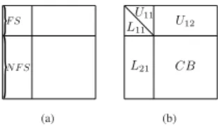
The multifrontal method was first introduced by Duff and Reid (1983). Being a direct method, it computes the solution of a sparse system Ax= b by means of a factorization of A un-der the form A= LU (in the unsymmetric case). This fac-torization is achieved through a sequence of partial factoriza-tions, performed on relatively small, dense matrices, called fronts. With each front are associated two sets of variables: the fully-summed (FS) variables, whose corresponding rows and columns of L and U are computed within the current front, and the non fully-summed (NFS) variables, which receive up-dates resulting from the elimination of FS variables. At the end of each partial factorization, the partial factors [L11L21] and[U11U12] are stored apart and a Schur complement referred to as a contribution block (CB) is held in a temporary memory area called CB stack, whose maximal size depends on several parameters. As the memory needed to store the factors is in-compressible (in full-rank), the CB stack can be viewed as an overcost whose peak has to be minimized. The structure of a front before and after partial factorization is shown in Fig. 1.
(a) (b)
Figure 1: A front before (a) and after (b) partial factorization.
The computational and memory requirements for the complete factorization strongly depend on how the fronts are formed and on the order in which they are processed. Reordering tech-niques such as nested dissection are used to ensure the
effi-ciency of the process: a tree, called elimination tree (Schreiber, 1982) is created, with a front associated with each of its nodes. Any post-order traversal of this tree gives equivalent properties in terms of factors memory and computational cost.
Block Low-Rank (BLR) matrices
A flexible, efficient technique can be used to represent fronts with low-rank subblocks based on a storage format called Block Low-Rank (BLR, see Amestoy et al. (2012)). Unlike other for-mats such as H -matrices (Hackbusch, 1999) and HSS matri-ces (Xia et al., 2009), the BLR one is based on a flat, non-hierarchical blocking of the matrix which is defined by con-veniently clustering the associated unknowns. A BLR repre-sentation of a dense matrix F is shown in equation (1) where we assume that p subblocks have been defined. Subblocks !Bi j of size mi j× ni jand numerical rank kεi jare approximated by a low-rank product Xi jYi jTat accuracy ε, when k
ε i j(mi j+ ni j) ≤ mi jni jis satisfied. ! F= ! B11 B!12 · · · B!1p ! B21 · · · ... .. . · · · ... ! Bp1 · · · B!pp (1)
In order to achieve a satisfactory reduction in both the com-plexity and the memory footprint, subblocks have to be chosen to be as low-rank as possible (e.g., with exponentially decay-ing sdecay-ingular values). This can be achieved by clusterdecay-ing the un-knowns in such a way that an admissibility condition (Beben-dorf, 2008) is satisfied. This condition states that a subblock
!
Bi j, interconnecting variables of i with variables of j, will have a low rank if variables of i and variables of j are far away in the domain, intuitively, because the associated variables are likely to have a weak interaction, as illustrated in Fig. 2(a). Subblocks which represent self-interactions (typically the di-agonal ones) are for this reason always full-rank. In practice, the subgraphs induced by the FS variables and the NFS vari-ables are algebraically partitioned with a suitable strategy.
80 100 120 140 160 180 200 0 10 20 30 40 50 60 70 80 90 100 128
distance between i and j
ran
k
of
ij
(a) (b)
Figure 2: (a) Correlation between distance from variables of i to variables of j and rank of block !Fi j. (b) Structure of a BLR front. The darkness of a block is proportional to its storage requirement (the lighter a block is, the smaller is its rank). Block Low-Rank multifrontal solver
A BLR multifrontal solver consists in approximating the fronts with BLR matrices, as shows Figure 2(b). BLR representations
of[L11U11], L21, U12and CB are computed separately. Note that in L21and U12, there are no self-interactions. The partial factorization is then adapted to benefit from the compressions using low-rank products instead of full-rank standard ones. An example of a BLR partial factorization algorithm is given in Algorithm 1. For sake of clarity, an unblocked version is pre-sented although this algorithm is, in practice, applied panel-wise with numerical pivoting.
Algorithm 1 Unblocked FSCU incomplete factorization of a front.
1: ◮Input: a front F
2: ◮Output: [L11L21], [U11U12] and a Schur comple-ment CB 3: 4: Factor ’F’: F11= L11[U11U12] 5: Solve ’S’: L21= F21U11−1 6: Compress ’C’: L21≃ X21Y21T ; U12≃ X12Y12T 7: Update ’U’: CB= F22− X21(Y21TY12)X12T
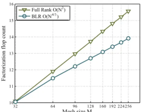
Although compression rates may not be as good as those achie-ved with hierarchical formats, BLR offers a good flexibility thanks to its simple, flat structure. Many variants of Algo-rithm 1 can be easily defined, depending on the position of the ’C’ phase. For instance, it can be moved to the last position if one needs an accurate factorization and an approximated, faster solution phase. This might be a strategy of choice for FWI application, where a large number of right-hand sides must be processed during the solution phase. In a parallel en-vironment, the BLR format allows for an easier distribution and handling of the frontal matrices. Pivoting in a BLR matrix can be more easily done without perturbing much the structure. Lastly, converting a matrix from the standard representation to BLR and vice versa, is much cheaper with respect to the case of hierarchical matrices (see Table 1 for the low global cost of compressing fronts into BLR formats). This allows to switch back and forth from one format to the other whenever needed at a reasonable cost; this is, for example, done to simplify the assembly operations that are extremely complicated to perform in any low-rank format. As shown in Fig. 3, the O(N2) com-plexity of a standard, full rank solution of a 3D problem (of N unknowns) from the Laplacian operator discretized with a 3D 11-point stencil is reduced to O(N4/3) when using the BLR format. All these points make BLR easy to adapt to any multi-frontal solver without a complete rethinking of the code.
NUMERICAL EXAMPLE
We perform acoustic finite-difference frequency-domain seis-mic modeling in the 3D SEG/EAGE overthrust model (Amin-zadeh et al., 1997) of dimension 20km× 20km × 4.65km with the 27-point mixed-grid finite-difference stencil (Operto et al., 2007) for the 2-Hz, 4-Hz and 8-Hz frequencies (Figures 4 and 5). Since we use a sequential prototype BLR solver, we per-form the simulation on a single 64-core AMD Opteron node equipped with 384GB of shared memory. We use single pre-cision arithmetic to perform the full-rank (FR) and the BLR factorizations. The point source is located at x (dip) = 2 km, y
32 64 96 128 160 192 224 256 10 11 12 13 14 15 16 Mesh size M F ac to ri za ti on fl op count
Full Rank O(N2) 4/3) BLR O(N
Figure 3: Flop scalability of the BLR multifrontal factorization of the Laplacian operator discretized with a 3D 11-point sten-cil, revealing a O(N4/3) complexity for ε = 10−14, N= M3.
(cross) = 2 km and z = 0.5 km. A discretization rule of 4-grid points per minimum wavelength leads to a grid interval of 250 m, 135 m and 68 m and a finite-difference grid of 0.3, 1.4 and 8 millions of nodes for the 2-Hz, 4-Hz and 8-Hz frequency, re-spectively, considering 8 grid points in the perfectly-matched layers surrounding the computational domain. The BLR solu-tions are computed for 3 values of the threshold ε (10−3, 10−4 and 10−5) and are validated against the FR solutions (Fig. 5(a-c)). The accuracy of the BLR solutions can be qualitatively as-sessed in Fig. 5(d-l) and the reduction of the memory demand and operation complexity resulting from the BLR approxima-tion are outlined in Table 1. The metrics provided in Table 1 are: [1] the flop count performed during the LU factorization and the overhead associated with the compression of the LU-factor (compressing LU-factors). [2] the memory for LU-LU-factor storage and the peak of CB stack used during the LU factor-ization, [3] the average reduction in size of the contribution blocks resulting from the BLR approximation. The metrics of the FR solver are absolute, while those of the BLR solver are given as a percentage of the metrics of the FR solver. In a first attempt to assess the footprint of the BLR approximation on seismic imaging, we show 2-Hz monochromatic reverse-time migrated images (RTM) computed from the FR and the BLR solutions in Figure 6. RTM is computed in the true velocity model for an array of shots and receivers near the surface with a shot and receiver spacings of 500 m and 250 m, respectively. BLR solutions for ε= 10−3are of insufficient quality for FWI applications (Fig. 5(d-f) and 6d), while those obtained with ε= 10−5closely match the FR solutions (Fig. 5(j-l) and 6b). BLR solutions for ε= 10−4show some slight differences with the FR solutions (Fig. 5(g-i)), but might be considered for FWI applications (Fig. 6c). For the 8-Hz frequency, the flop count performed during the BLR factorization represents 14.8% (ε= 10−4) and 21.3% (ε= 10−5) of the one performed during the FR factorization. It is worth noting that the flop-count reduc-tion increases with frequency (i.e., with the size of the com-putational grid) as the maximum distance between variables in the grid increases (Fig. 2), a key feature in view of larger-scale simulations. For example, for ε= 10−4, the flop count decreases from 24.8% to 14.8% when the frequency increases from 2 Hz to 8 Hz. The overhead associated with the
decom-pression of the contribution block is negligible, a distinct ad-vantage compared to the HSS approach of Wang et al. (2011), and hence should not impact significantly the performance of the BLR factorization. The memory saving achieved during the BLR factorization follows the same trend than the flop count, as it increases with frequency. For the 8-Hz frequency and ε= 10−5, the memory for LU-factor storage and the peak oF CB stack during BLR factorization represent 41.6% and 23.9% of those required by the FR factorization, respectively (Table 1). The reduction of the storage of the contribution blocks (CB) is even higher. Both (LU and CB compression) will contribute to reducing the volume of communication by a substantial factor and improving the parallel efficiency of the solver. 0 1 2 3 4 Depth (km) 0 Dip (km) 5 10 15 20 Cross (km) 5 10 15 20 3000 4000 m/s 5000 6000
Figure 4: SEG/EAGE overthrust velocity model.
CONCLUSION
We have presented applications of a new Block Low-Rank (BLR) algebraic sparse direct solver for frequency-domain seis-mic modeling. The computational time and memory savings achieved during BLR factorization increase with the size of the computational grid (i.e., frequency), suggesting than one order of magnitude of saving for these two metrics can be viewed for large-scale factorization involving several tens of millions of unknowns. Future work involves implementation of MPI parallelism in the BLR solver and a sensitivity analysis of FWI to the BLR approximation before application of visco-acoustic FWI on wide-azimuth data recorded with fixed-spread acquisition geometries (Brossier et al., 2013). The computa-tional efficiency of the BLR solver might still be improved by iterative refinement of the solutions (although this refine-ment needs to be performed for each right-hand side) and/or by performing the BLR factorization in double precision. The computational savings provided by the BLR solver might al-low to view frequency-domain seismic modeling in realistic 3D visco-elastic anisotropic media (Wang et al., 2012).
ACKNOWLEDGMENTS
This study was funded by the SEISCOPE consortium (http://seiscope.oca.eu) and by EDF under collaboration contract 8610-AAP-5910070284.
F Flop count LU Mem LU Peak memory Flop count(%) (BLR) Compressing factors (BLR) (FR) (FR) (FR) ε= 10−3 ε= 10−4 ε= 10−5 ε= 10−3 ε= 10−4 ε= 10−5
2 8.957E+11 3 GB 6 GB 21.1 24.8 36.6 3.5 4.5 5.2
4 1.639E+13 22 GB 25 GB 12.7 18.6 25.6 1.1 1.4 1.8
8 5.769E+14 247 GB 445 GB 9.5 14.8 21.3 0.3 0.4 0.5
F Mem LU(%) (BLR) Peak of CB stack(%) (BLR) Average storage CB(%) (BLR) ε= 10−3 ε= 10−4 ε= 10−5 ε= 10−3 ε= 10−4 ε= 10−5 ε= 10−3 ε= 10−4 ε= 10−5
2 44.7 53.4 61.8 16.8 23.9 32.3 30.9 41.1 51.1
4 34.5 42.2 50.0 19.0 21.7 24.4 20.7 29.3 38.1
8 21.3 28.9 41.6 15.9 19.4 23.9 15.0 22.5 30.3
Table 1: Statistics of the Full-Rank (FR) and Block Low-Rank (BLR) simulations. F(Hz): modeled frequency. Flop count: number of flops during LU factorization. Mem LU: Memory for LU factors in GigaBytes. Peak of CB stack: Maximum size of CB stack during LU factorization in Gigabytes. The metrics (flops and memory) for the low-rank factorization are provided as percentage of those required by the full-rank factorization (first 3 columns - top row).
0 1 2 3 4 Depth (km) 0 Dip (km) 5 10 15 20 Cross (km ) 5 10 15 20 0 1 2 3 4 Depth (km) 0 Dip (km) 5 10 15 20 Cross (km) 5 10 15 20 0 1 2 3 4 Depth (km) 0 Dip (km) 5 10 15 20 Cross (km) 5 10 15 20 0 1 2 3 4 Depth (km) 0 Dip (km) 5 10 15 20 Cross (km) 5 10 15 20 0 1 2 3 4 Depth (km) 0 Dip (km) 5 10 15 20 Cross (km) 5 10 15 20 0 1 2 3 4 Depth (km) 0 Dip (km) 5 10 15 20 Cross (km) 5 10 15 20 b) c) 0 1 2 3 4 Depth (km) 0 Dip (km) 5 10 15 20 Cross (km) 5 10 15 20 0 1 2 3 4 Depth (km) 0 Dip (km) 5 10 15 20 Cross (km) 5 10 15 20 0 1 2 3 4 Depth (km) 0 Dip (km) 5 10 15 20 Cross (km) 5 10 15 20 0 1 2 3 4 Depth (km) 0 Dip (km) 5 10 15 20 Cross (km) 5 10 15 20 0 1 2 3 4 Depth (km) 0 Dip (km) 5 10 15 20 Cross (km) 5 10 15 20 0 1 2 3 4 Depth (km) 0 Dip (km) 5 10 15 20 Cross (km) 5 10 15 20 a) d) e) f) g) h) i) j) k) l) a)
Figure 5: (a-c) Full-rank solution (real part). (a) 2 Hz, (b) 4 Hz, (c) 8 Hz. (d-f) Difference between full-rank and low-rank solutions for ε= 10−3. (d) 2 Hz, (e) 4 Hz, (f) 8 Hz. (g-i) Same as (d-f) for ε= 10−4. (j-l) Same as (d-f) for ε= 10−5. Amplitudes are clipped to half the mean amplitude of the full-rank wavefield on each panel.
0 1 2 3 4 Depth (km) 0 Dip (km) 5 10 15 20 Cross (km) 5 10 15 20 0 1 2 3 4 Depth (km) 0 Dip (km) 5 10 15 20 Cross (km) 5 10 15 20 0 1 2 3 4 Depth (km) 0 Dip (km) 5 10 15 20 Cross (km) 5 10 15 20 0 1 2 3 4 Depth (km) 0 Dip (km) 5 10 15 20 Cross (km) 5 10 15 20 a) b) c) d)
REFERENCES
Amestoy, P., C. Ashcraft, O. Boiteau, A. Buttari, J.-Y. L’Excellent, and C. Weisbecker, 2012, Improving multifrontal methods by means of block low-rank representations: Rapport de recherche RT/APO/12/6, INRIA/RR-8199, Institut National Polytechnique de Toulouse, Toulouse, France. Submitted for publication in SIAM Journal on Scientific Computing.
Aminzadeh, F., J. Brac, and T. Kunz, 1997, 3-D Salt and Overthrust models: SEG/EAGE 3-D Modeling Series No.1.
Bebendorf, M., 2008, Hierarchical matrices: A means to efficiently solve elliptic boundary value problems (lecture notes in com-putational science and engineering): Springer, 1 edition.
Ben-Hadj-Ali, H., S. Operto, and J. Virieux, 2008, Velocity model building by 3d frequency-domain, full-waveform inversion of wide-aperture seismic data: Geophysics, 73, WE101–WE117.
Brossier, R., V. Etienne, G. Hu, S. Operto, and J. Virieux, 2013, Performances of 3D frequency-domain full-waveform inver-sion based on frequency-domain direct-solver and time-domain modeling: application to 3D OBC data from the Valhall field: International Petroleum Technology Conference, Beijing, China, IPTC 16881.
Brossier, R., V. Etienne, S. Operto, and J. Virieux, 2010, Frequency-domain numerical modelling of visco-acoustic waves based on finite-difference and finite-element discontinuous galerkin methods, in Dissanayake, D. W., ed., Acoustic Waves, 125–158. SCIYO.
Duff, I. S., A. M. Erisman, and J. K. Reid, 1986, Direct methods for sparse matrices: Clarendon Press.
Duff, I. S. and J. K. Reid, 1983, The multifrontal solution of indefinite sparse symmetric linear systems: ACM Transactions on Mathematical Software, 9, 302–325.
George, A. and J. W. Liu, 1981, Computer solution of large sparse positive definite systems: Prentice-Hall, Inc.
Hackbusch, W., 1999, A sparse matrix arithmetic based on H -matrices. Part I: Introduction to H -matrices: Computing, 62, 89–108.
Marfurt, K., 1984, Accuracy of finite-difference anf finite-element modeling of the scalar and elastic wave equations: Geophysics, 49, 533–549.
Operto, S., J. Virieux, P. Amestoy, J.-Y. L’ ´Excellent, L. Giraud, and H. Ben Hadj Ali, 2007, 3D finite-difference frequency-domain modeling of visco-acoustic wave propagation using a massively parallel direct solver: A feasibility study: Geophysics, 72, SM195–SM211.
Pratt, R. G., 1999, Seismic waveform inversion in the frequency domain, part I : theory and verification in a physic scale model: Geophysics, 64, 888–901.
Schreiber, R., 1982, A new implementation of sparse Gaussian elimination: ACM Transactions on Mathematical Software, 8, 256–276.
Toks¨oz, M. N. and D. H. Johnston, 1981, Geophysics reprint series, no. 2: Seismic wave attenuation: Society of exploration geophysicists.
Virieux, J. and S. Operto, 2009, An overview of full waveform inversion in exploration geophysics: Geophysics, 74, WCC1– WCC26.
Wang, S., M. V. de Hoop, and J. Xia, 2011, On 3d modeling of seismic wave propagation via a structured parallel multifrontal direct helmholtz solver: Geophysical Prospecting, 59, 857–873.
Wang, S., M. V. de Hoop, J. Xia, and X. S. Li, 2012, Massively parallel structured multifrontal solver for time-harmonic elastic waves in 3D anisotropic media: Geophysical Journal International, 191, 346–366.
Xia, J., S. Chandrasekaran, M. Gu, and X. S. Li, 2009, Superfast multifrontal method for large structured linear systems of equa-tions: SIAM Journal on Matrix Analysis and Applications, 31, 1382–1411.