Multidimensional Ultrasound Doppler Signal Analysis for Fetal Activity Monitoring

To link to this article :

DOI: 10.1016/j.ultrasmedbio.2015.07.026

URL :

http://dx.doi.org/10.1016/j.ultrasmedbio.2015.07.026

To cite this version :

Ribes, Sophie and Girault, Jean-Marc and

Perrotin, Franck and Kouamé, Denis Multidimensional Ultrasound

Doppler Signal Analysis for Fetal Activity Monitoring. (2015)

Ultrasound in Medicine and Biology, vol. 41 (n° 12). pp. 3172-3181.

ISSN 0301-5629

O

pen

A

rchive

T

OULOUSE

A

rchive

O

uverte (

OATAO

)

OATAO is an open access repository that collects the work of Toulouse researchers and

makes it freely available over the web where possible.

This is an author-deposited version published in :

http://oatao.univ-toulouse.fr/

Eprints ID : 15388

Any correspondence concerning this service should be sent to the repository

administrator:

staff-oatao@listes-diff.inp-toulouse.fr

MULTIDIMENSIONAL ULTRASOUND DOPPLER SIGNAL ANALYSIS FOR FETAL

ACTIVITY MONITORING

S

R

,

*

J

-M

G

,

F

P

,

and D

K

!

*

* University of Toulouse III, IRIT UMR CNRS 5505, Toulouse, France;y_{University of Tours, INSERM U930 Tours, France; and} z_{CHU Bretonneau, Tours, service de Gynecologie Obst!etrique, INSERM U930, Tours, France}

Abstract—Fetal activity parameters such as movements, heart rate and the related parameters are essential indi-cators of fetal wellbeing, and no device provides simultaneous access to and sufficient estimation of all of these pa-rameters to evaluate fetal health. This work was aimed at collecting these papa-rameters to automatically separate healthy from compromised fetuses. To achieve this goal, we first developed a multi-sensor–multi-gate Doppler sys-tem. Then we recorded multidimensional Doppler signals and estimated the fetal activity parameters via dedicated signal processing techniques. Finally, we combined these parameters into four sets of parameters (or four hyper-parameters) to determine the set of parameters that is able to separate healthy from other fetuses. To validate our system, a data set consisting of two groups of fetal signals (normal and compromised) was established and provided by physicians. From the estimated parameters, an instantaneous Manning-like score, referred to as the ultrasonic score, was calculated and was used together with movements, heart rate and the associated parameters in a clas-sification process employing the support vector machine method. We investigated the influence of the sets of pa-rameters and evaluated the performance of the support vector machine using the computation of sensibility, specificity, percentage of support vectors and total classification error. The sensitivity of the four sets ranged from 79% to 100%. Specificity was 100% for all sets. The total classification error ranged from 0% to 20%. The percentage of support vectors ranged from 33% to 49%. Overall, the best results were obtained with the set of parameters consisting of fetal movement, short-term variability, long-term variability, deceleration and ul-trasound score. The sensitivity, specificity, percentage of support vectors and total classification error of this set were respectively 100%, 100%, 35% and 0%. This indicated our ability to separate the data into two sets (normal fetuses and pathologic fetuses), and the results highlight the excellent match with the clinical classification per-formed by the physicians. This work indicates the feasibility of detecting compromised fetuses and also represents an interesting method of close fetal monitoring during the entire pregnancy. (E-mail:kouame@irit.fr)

Key Words: Fetal monitoring, Fetal heart rhythm, Fetal movement, Multidimensional signals, Support vector machine.

INTRODUCTION

Fetal monitoring may be required at different times dur-ing pregnancy to closely monitor certain fetal and maternal disorders (Manning et al. 1980). Existing methods, which consist of asking women to count the number of fetal movements, performing a biophysical profile or Manning’s test (Manning et al. 1980) or analyzing general movements, may be either subjective or time consuming. To automatically monitor fetal activ-ity, the most commonly used system is the cardiotoco-gram. This device measures fetal heart rate (FHR) and

uterine contractions (Royal College of Obstetricians

and Gynecologists [RCOG] 2001) but does not provide

any information regarding fetal movements. This may explain why the performances of major classifiers, which are based on FHR variability analysis alone (through different kind of entropies), are on the order of 80% for specificity and 80% for sensitivity (Ferrario et al. 2006). We believe that additional information may improve classification performance. There are many dedicated ultrasound systems that collect additional in-formation such as fetal movement and pseudo-breathing. Unfortunately, these systems provide only partially automated detection of fetal movement

(Karlsonn et al. 2000a) or breathing (Karlsonn et al.

Some preliminary attempts to overcome these limi-tations were made by Krib"eche et al. (2007). The main characteristic of their system is that, because of the large number of sensors needed to cover an explored area as large as possible, a large number of Doppler signals have to be processed. The aim of our work was not to develop new signal processing methods and evaluate their performance. Instead, we sought to efficiently combine some relevant existing signal processing techniques to achieve the following goals: extract fetal activity features, such as FHR and movements (and related features), and efficiently collect these features to differentiate between normal and potentially compromised fetuses. To achieve these goals, we needed first to reduce the inherent redun-dancy related to the large number of acquired Doppler signals and then to separate fetal from maternal signals through a blind source separation. The detailed signal processing algorithms used to extract the fetal activity pa-rameters are not detailed here. The reader is referred to, for example, Rouvre et al. (2005), Voicu (2011) and

Voicu et al. (2010, 2014). However, even if the number

of relevant data can be reduced, a fusion step is required to provide the physical with global information, for example, an ‘‘ultrasound score,’’ on which a decision can be based.

Thus, the main challenge of this study, and its incre-mental value with respect to the previously published article (Krib"eche et al. 2007), was to develop a method that enables extraction of the relevant information neces-sary to construct a global indicator sufficiently pertinent to classify fetuses into normal and potentially compro-mised groups. To validate the feasibility, this method was successfully tested on a heterogeneous data set ob-tained from pregnant women and composed of FHR, movement and pseudo-breathing signals. To our knowl-edge, this automated classification is a new and important contribution to the search for an objective method for monitoring fetal activity, which remains an open issue

(Grivell et al. 2010; Kaluzynskia et al. 2011).

This article is arranged as follows: We first described the device produced by an industrial collaboration and used for this study, and then briefly introduce the signal processing techniques used. The ultrasound score is then introduced and investigated using fetal activity pa-rameters obtained from real fetal Doppler signals. Finally, results from classification of sets of fetuses are discussed.

MATERIALS AND METHODS Materials

We constructed, in collaboration with Althais Tech-nologies (Tours, France), a multi-sensor Doppler system (Surfoetus) that was able to monitor most parts of the fetal

body. Although a complete description of the develop-ment of this device is beyond the scope of this article, we briefly provide here a brief description. The system consists of 12 ultrasound (US) sensors, each with five gates, working at a frequency of f_{05 2 MHz and an} elec-tronic US device (three elecelec-tronic pulsed Doppler boards and one data acquisition board). A low-noise amplifier amplifies the received signal; a deep compensated ampli-fier then balances the strong attenuation of the deepest gates. After complex demodulation and filtering, the Doppler components are sampled sequentially and con-verted. Sampling frequency, denoted Fe, is 1 kHz. Five

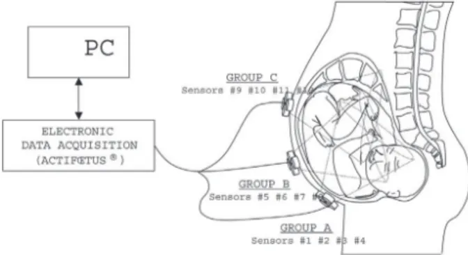
adjustable gates ranging from 2 to 14 cm are used to explore the depths. These 12 sensors are divided into three groups of four sensors, as illustrated in Figure 1. Group A (US sensors 1–4) is used to explore the fetal tho-rax, investigating FHR and breathing movements; group B (sensors 5–8) the upper limbs; and group C (sensors 9–12) the lower limbs. Each sensor is a circular piezo-electric element 12 mm in diameter. The ultrasound beam was not focused. A belt was used during recording to maintain all three groups.

Protocol

In this study, 44 pregnant women at a gestational age .24 weeks were prospectively enrolled. Inclusion criteria were singleton pregnancy, absence of significant maternal complications requiring premature delivery (hy-pertensive disorders; renal, heart or immunologic pathol-ogy; pre-existing diabetes), willingness to have pregnancy followed or delivered locally, maternal age .18 years and health insurance affiliation. Exclusion criteria were fetal malformation, maternal significant complications, pregnancy care in another center and concomitant participation in another research protocol. This study was approved by the University’s ethics committee (Clinical Investigation Centre, Innovation

Fig. 1. Sensor group arrangement. Group A (sensors 1–4) ex-plores the fetal thorax, investigating fetal heart rate and breath-ing movements. Group B (sensors 5–8) explores the upper limbs, and group C (sensors 9–12), the lower limbs. A belt is

Technology, Ethics). The ethics ID number was 2004-32, and the study number was CT04-SURFOETUS. All par-ticipants submitted a signed informed consent.

The standard demographic measures, expressed as the mean 6 standard deviation (range) were age 5 29.9 6 5.9 (20–44) years, height 5 164 6 6 (151–179) cm and weight 5 63.23 6 15.88 (41–123) kg. Pregnancies were classified in two groups: normal and IUGR (intra-uterine growth restriction) depending on ultrasound-estimated fetal growth at inclusion. IUGR was defined as an estimated fetal weight under the 10th percentile or a transverse abdominal perimeter below the 10th percentile for gestational age. All recordings were per-formed between the 24th and 40th weeks of gestation in the Obstetrics Department of Bretonneau University Hos-pital, Tours, France. In the ‘‘normal’’ group, recordings were performed every 4 weeks, and in the ‘‘IUGR’’ group, recordings were performed every 2 weeks. The overall mean gestational age was 30.2 weeks (median 5 32 weeks). The mean gestational age of the normal group was 30.1 weeks, and the mean gestational age of the IUGR group was 29.9 weeks.

Overall, we obtained 98 Doppler signals for the 44 patients. Each examination in this protocol was 30 min long. The first group, referred to as ‘‘normal pregnan-cies,’’ consisted of 74 measurements and 31 subjects. The second group, referred to as ‘‘pathologic pregnan-cies’’ or ‘‘group with IUGR’’ consisted of 24 measure-ments and 13 subjects.

Procedures

As mentioned earlier, the electronic control system is composed of 12 sensors with five gates per sensor, and thus, 60 complex Doppler signals must be processed each millisecond. This is a very large amount of data with inevitable redundancy in the signals. Furthermore, as the signals recorded from different sensors originate from different sources of signals (fetal heart movement, maternal heart movement, respiration, etc.), a source sep-aration is strongly expected to extract fetal signal only. Assuming that there is an L-dimensional zero-mean signal source vector s_{ðtÞ 5 ½s}1ðtÞ; .; sLðtÞ&T, and an

M-dimen-sional data vector x_{ðtÞ 5 ½x}1ðtÞ; .; xMðtÞ&T observed at

each time point t. In short, L is the number of sources, and M is the number of observable mixed data. L and M are generally different. These signals can be modeled as

xðtÞ 5 A:sðtÞ1uðtÞ (1) where x represents the signals observed or acquired by the sensors, referred to below as the ‘‘observation matrix’’; A is the mixing matrix, corresponding to maternal body ‘‘mixing’’; s is the unobservable source matrix; and u(t) is a zero-mean Gaussian noise vector with a covariance

matrix L. In summary, we have different source signals denoted s non-observable, which are mixed and acquired by the sensors and denoted x. As stated before, the fetal signals need to be extracted and separated to correctly monitor fetal activity. To perform an unsupervised source separation, that is, without any a priori information, the number of independent sources must be evaluated from our data set. To do so in a parsimonious way, a redun-dancy information reduction must be performed. Dimension reduction and sparse blind source separation

From the set of data, we perform dimension reduc-tion to eliminate the data redundancy (see Appendix A). We searched for the number of independent sources using the method described inAppendix A. This number of independent sources was found to be two or three. Knowing the number of sources, we performed signal separation to separate the fetal Doppler signal from the mother’s signal (seeAppendix B). The last technique to be explored concerned the statement of a meta-descriptor allowing an objective evaluation of fetal state. Ultrasound score

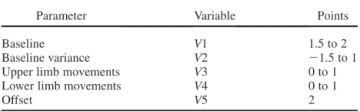
To compute an objective parameter including infor-mation on fetal heart rate and fetal movements, we intro-duced a Manning-like hyper-parameter referred to as the ultrasound score (Ribes et al. 2011). This meta-descriptor was computed every minute during each examination, as explained later. The ultrasound score is the sum of five values denoted V1, V2, V3, V4 and V5 that are based on the estimated fetal activity parameters, as reported in

Table 1.

V1 and V2 were both based on the fetal heart rate, which is an essential component in the follow-up of preg-nancies (Rouvre et al. 2005; Voicu et al. 2010) because it is correlated with fetal health. As reported inTable 1, V1 represents the baseline (or mean value of FHR), and V2 represents the variance of the baseline. This baseline is the mean FHR computed when the variability was bet-ween 5 and 25 bpm over 1 minute. The baseline is rounded to increments of 5 bpm during a 10-min segment. The normal value lies between 110 and 160 bpm. Detec-tion of the FHR may be improved using a specific prior

(Manning 1977).

Table 1. Ultrasound score: Parameters computed each minute, associated variables and resulting points

Parameter Variable Points

Baseline V1 1.5 to 2

Baseline variance V2 _{21.5 to 1}

Upper limb movements V3 0 to 1

Lower limb movements V4 0 to 1

V3 and V4 are both based on limb movements. V3 represents upper limb movements whereas V4 represents lower limb movements. These movements can be de-tected either on the separated magnitudes by their sudden changes or by searching for the increase or decrease in the overall phase. However, to eliminate false detection caused by phase noise, detection of fetal movement was combined with a threshold algorithm (Karlsonn et al.

2000b). In this algorithm a movement was defined by a

magnitude level above the noise threshold with a mini-mum duration of 0.2 s, followed by a minimini-mum rest dura-tion of 0.5 s.

Finally, V5 is an offset.

The empirical range of values was chosen on the following basis:

' If the baseline was .110 or ,160 bpm, the value of V1 was set between 1.5 and 2; otherwise V1 was set at 0. More precisely, let BL denote the baseline. Thus, V1 is defined as V1 5 0:01ðBL2110Þ11:5 if 110#BL#160; V1 5 0 otherwise.

' If the baseline variance was ,17.5, then the value of V2 was set between 0 and 1; if the baseline variance was .17.5, but ,22.5, then the value of V2 was set be-tween 21.5 and 1; otherwise, the value of V2 was set at 21.5. More precisely, let BLV denote the baseline variance (which is a positive value). Thus V2 is defined

by V2 5 BLV=17:5 if 0#BLV#17:5;

V2 5 20:5ðBLV217:5Þ11 if 17:5,BLV#22:5; and V2 5 21:5 if BLV.22:5.

' If two or more upper limb movements were detected, the value of V3 was set at 1; otherwise V3 was set at 0. If two or more lower limb movements were detected, then the value of V4 was set at 1; otherwise the value of V4 was set to 0.

' To have a positive ultrasound score, we added an offset through V5 which is set at 2.

The ultrasound score for the complete recording was the mean of the ultrasound score computed for each

min-ute. Figure 2 illustrates an example of the ultrasound

score. At the top are the mean FHR and the standard de-viation for each minute. In the middle are the numbers of movements detected from the upper limbs (blue) and lower limbs (magenta). At the bottom is the ultrasound score calculated from the aforementioned parameters.

As the parameters do not have the same importance in the follow-up of fetal well-being, we investigated different sets of parameters through four new parameters referred to as hyper-parameters:

' Hyper-parameter 1 consisted of baseline, fetal move-ment and ultrasound score.

' Hyper-parameter 2 consisted of baseline, fetal move-ment, short-term variability and ultrasound score.

' Hyper-parameter 3 consisted of baseline, fetal move-ment and short-term variability.

' Hyper-parameter 4 consisted of fetal movement, short-term variability, long-short-term variability, deceleration and ultrasound score.

Note that variability is the fluctuation in the FHR, quantified as the amplitude peak-to-peak trough in beats per minute. Short-term variability (STV) of FHR is commonly used in prediction of fetal distress. STV is the oscillation of the FHR around the baseline in ampli-tudes of 5 to 25 bpm, measured on time windows of 3.75 s. Long-term variability is the mean value over a minute (i.e., the difference between the highest and the lowest values of FHR).

Recall of used support vector machine method

To find the best hyper-parameter, we propose the use of support vector machine (SVM) classification. Different classification methods were evaluated (Duda

et al. 2001), and the SVM method (Ferrario et al.

1999; Vapnik 1995) was better able to classify the

current data. To ensure a better understanding, the principles of SVM classification are provided in

Appendix C. In this study and using SVM principles,

a score optimization problem can be reformulated as a classification problem. The problem under consideration was the study of the separability of the data (normal fe-tuses vs. compromised fefe-tuses), using only estimation of the hyper-parameters mentioned earlier. We had a clas-sification problem in which the kernel function, the set of hyper-parameters, the kernel function features and the value of the constraint C had to be chosen. The choice of kernel functions was studied empirically, and optimal results were achieved using a polynomial kernel function defined by

Kðx; x0_{Þ 5 ð11x:x0Þ}d

(2) where d is the degree defined by the user. To obtain the best results, the SVM was computed using a polynomial kernel function for different sets of hyper-parameters, kernel degrees and a constraint C defined by the user.

First, the data was pre-processed to separate the sig-nals of the mothers from those of the fetuses, and then the parameters listed in Table 1were computed. The effec-tiveness of the SVM classification was evaluated using the computation of specificity, sensitivity, percentage of support vectors and total classification accuracy defined as follows:

' Specificity is the number of true-negative decisions divided by the number of normal pregnancies. ' Sensitivity is the number of true-positive decisions

' Percentage of support vectors is the number of support vectors divided by the number of pregnancies. ' Classification accuracy is the number of correct

deci-sions divided by the number of pregnancies.

A true-negative decision occurred when the classi-fier and the physician suggested the absence of positive detection. A true-positive decision occurred when the classifier and the physician suggested a positive

Fig. 2. Top: Mean fetal heart rate and mean STV each minute. Middle: Number of movements of the upper limbs (blue) and lower limbs (purple). Bottom: Ultrasound score calculated according to parameters. FHR 5 fetal heart rate; STV 5

detection. As mentioned previously, a binary clinical classification (normal pregnancies and pregnancies asso-ciated with IUGR disorders) was performed by physicians.

RESULTS

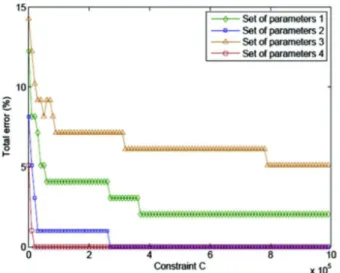
We first searched for the best hyper-parameter. For different kernel degrees d and different constraints C, we performed the classification process and compared classification accuracies.Figure 3illustrates the relation-ship between total error and constraint for the different hyper-parameters: for all hyper-parameters, total error decreased when constraint C increased. Hyper-parameters 2 and 3 differed only by consideration of the ultrasound score, and hyper-parameter 2, which con-tained this parameter, always yielded greater accuracy than hyper-parameter 3, confirming that inclusion of the ultrasound score facilitated and improved the classifica-tion process. For all constraint C values, hyper-parameter 4 always yielded the best results, and we chose to investigate only this hyper-parameter in the remainder of our study.

To find the optimal degree of the polynomial kernel function, we evaluated the performance of the classifica-tion considering hyper-parameter 4 and increasing constraint C for different degrees, as illustrated in

Figure 4. Higher degrees offered more general solutions,

with a reduction in the number of support vectors, projec-ting data into a higher-dimensional space and providing a lower error rate. At the same time, if we chose to use high levels of constraint C, we obtained better classification accuracy. The traoff between the complexity of the de-cision region and the training error rate can be monitored by changing parameter C.

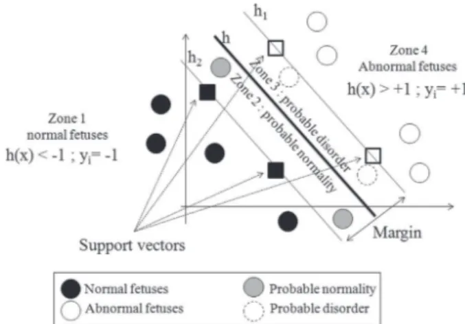
Once the effects of the degree, constraint and set of hyper-parameters had been studied, the results summa-rized inTables 2and3were obtained for a degree value d 5 15 and a constraint value C 5 9.0 3 105 for all sets of hyper-parameters.Table 2outlines the distribution of normal pregnancies, and Table 3, the distribution of pregnancies that presented with IUGR disorders. Zones 1–4, revealed by the classifier, corresponded to areas related to the hyper-planes found, as illustrated in

Figure 5. Zones 1 and 4 are the areas in which the fetuses

were classified without any doubt as normal and compro-mised, respectively. Zones 2 and 3 provided trends and were associated with probable normality for zone 2 and probable compromise for zone 3. It can be seen in

Table 2, for all sets of hyper-parameters, that the normal

pregnancies were found only in zones 1 and 2, that is, in the zones of normality. InTable 3, for the sets of hyper-parameters 2 and 4, it can be seen that no pregnancy was classified in zones 1 and 2; there were no false-negative decisions. From these two tables, we can

Fig. 3. Comparison of the total error for all hyper-parameters and various constraints for a degree value d 5 15.

Hyper-parameter 4 was always better.

Fig. 4. For various values of constraints and various degrees of kernel, the total error made for hyper-parameter 4 is evaluated.

High degrees and high constraints provided better results.

Table 2. Distribution of normal pregnancies, polynomial kernel function, degree d 5 15, constraint C 5 9.0 3

105* Zone Hyper-parameter 1 2 3 4 1 75.67% 68.91% 64.86% 68.91% 2 24.32% 31.08% 35.13% 31.08% 3 0 0 0 0 4 0 0 0 0

* Zones 1–4 were provided by the classifier and corresponded to a location related to the three hyperplanes. Zones 1 and 4 were the zones where the fetuses were clearly classified as normal fetuses and as fetuses presenting intrauterine growth retardation disorders, respectively. Zones 2 and 3 provided trends and were associated with probable normality for zone 2 and probable disorder for zone 3.

conclude that hyper-parameters 1–4 can identify all normal pregnancies (Table 2), and hyper-parameters 2 and 4 can identify all pregnancies that present with an IUGR disorder (Table 3).

It should be noted that we were able to identify all normal pregnancies (Table 2) and all pathologic pregnan-cies (Table 3), and these were good results concerning the separability of the data. Table 4provides the overall re-sults using evaluation of sensitivity and specificity. It can be seen that all sets of hyper-parameters, including the ultrasound score, yielded better results. Sensitivity, specificity and total error rate were excellent for hyper-parameters 2 and 4, which confirms the separability of the data in a high-dimensional space. According to the percentage of support vectors, we suggest use of hyper-parameter 4, which used fewer support vectors during the learning stage. Note also that the specificity and sensi-tivity values included the support vector.

DISCUSSION AND CONCLUSIONS

We have illustrated in this work that combining some efficient and dedicated signal processing techniques for extraction of fetal activity features (fetal heart rhythm, variabilities, fetal limb, accelerations) can enable close separation of normal from compromised fetuses. To do so we introduced an ultrasound score, including the pa-rameters fetal heart rate value, short-term variability and numbers of movements of the upper and lower limbs. We combined this score and other fetal activity parame-ters to obtain different hyper-parameparame-ters. Using these hyper-parameters and a SVM classification method, we illustrated the ability of our system to separate data into two sets, normal pregnancies and pathologic pregnancies, and obtained excellent matches to clinical classifications performed by physicians. These are valuable results and indicate an interesting way forward for home fetal moni-toring. To our knowledge, this system is unique.

This study had two main limitations that will be investigated in our future works: binary classification and limited validation. With respect to binary classifica-tion, we considered here two groups (normal and IUGR). Different types of pathologies and subgroups of pathologies, with different stages, could be valuable in testing the robustness of our method. As for limited vali-dation, the study was performed in a single clinical center. Using data from different clinical centers and performing classification of new and independent data would also help to enhance the validity of the methods on a large scale.

Acknowledgments—This study was supported by the Agence Nationale de la Research (Project ANR-07-TECSAN-023, Surfoetus) and per-formed with CIC-IT 1415, Tours. We warmly thank Laurent Colin, Phil-ippe Vince, Fabrice Gens and Thierry Pottier from Althias University of Tours, Tours, France; Catherine Roussel and Morgane Fournier-Massignan from CHU Bretonneau Tours, France; and Dr. Iulian Voicu.

REFERENCES

Attias H. Independent factor analysis. Neural Comput 1999;11: 803–851.

Bingham E, Hyvarinen A. A fast fixed-point algorithm for independent component analysis of complex valued signals. Int J Neural Syst 2000;10:1–8.

Table 3. Distribution of the pregnancies presenting with disorders, polynomial kernel function, degree d 5 15,

constraint C 5 9.0 3 105* Zone Hyper-parameter 1 2 3 4 1 4.16% 0 8.33% 0 2 4.16% 0 12.5% 0 3 50% 58.33% 70.83% 50 4 41.66% 41.66% 8.33% 50

* Zones 1–4 were provided by the classifier and corresponded to loca-tion related to the three hyperplanes. Zones 1 and 4 were the zones where the fetuses were clearly classified as normal fetuses and as fetuses pre-senting with intrauterine growth retardation disorders, respectively. Zones 2 and 3 provided trends and were associated with probable normality for zone 2 and probable pathology for zone 3.

Fig. 5. Support vector machine classification. Zones 1–4 are provided by the classifier and correspond to areas related to the hyperplanes. Zones 1 and 4 are the areas where the fetuses were classified respectively as normal fetuses and as abnormal fetuses. Zones 2 and 3 provide respectively trends of probable

normality and probable disorder.

Table 4. Overall evaluation: the total error, the percentage of support vectors, the sensitivity and the

specificity were computed for all hyper-parameters

Hyper-parameter 1 2 3 4 Total error 20.4% 0 5.1% 0 Support vectors 32.65% 37.75% 48.97% 35.71% Sensitivity 91.66% 100% 79.16% 100% Specificity 100% 100% 100% 100%

Cardoso JF. Blind signal separation: Statistical principles. Proc IEEE 1998;9:2009–2025.

Cardoso JF. Higher-order contrasts for independent component analysis. Neural Comput 1999;11:157–192.

Davis M, Mitinoudis N. A simple mixture for sparse overcomplete ICA. IEE Proc Vision Image Signal Process 2004;151:35–43.

Duda R, Hart P, Stork D. Pattern classification. 2nd ed. New York: Wi-ley; 2001.

Ferrario M, Signorini MG, Magenes G, Cerutti S. Support-vector net-works. Mach Learn 1999;20:273–297.

Ferrario M, Signorini MG, Magenes G, Cerutti S. Comparison of entropy-based regularity estimators: Application to the fetal heart rate signal for the identification of fetal distress. IEEE Trans Biomed Eng 2006;53:119–125.

Grivell R, Alfirevic Z, Gyte G, Devane D. Antenatal cardiotocography for fetal assessment (review). Cochrane Database Syst Rev 2010; 1:CD007863.

Ikeda S, Toyama K. Independent component analysis for noisy data: MEG data analysis. Neural Netw 2000;13:1063–1074.

Kaluzynskia K, Kreta T, Czajkowskib K, Sienkob J, Zmigrodzkia J. Sys-tem for objective assessment of fetal activity. Med Eng Phys 2011; 33:692–699.

Karlsonn B, Berson M, Helgason T, Geirsson R, Pourcelot L. Effect of fetal and maternal breathing on the ultrasonic Doppler signal due to fetal heart movement. Eur J Ultrasound 2000a;11:47–52. Karlsonn B, Foulqui"ere K, Kaluzynski K, Tranquart F, Fignon A,

Pourcelot D, Pourcelot L, Berson M. The Dopfet system: A new ul-trasonic Doppler system for monitoring and characterisation of fetal movement. Ultrasound Med Biol 2000b;26:1117–1124.

Krib"eche A, Tranquartlow F, Kouame D, Pourcelot L. The Actifetus sys-tem: A multidoppler sensor system for monitoring fetal movements. Ultrasound Med Biol 2007;33:430–438.

Lee TW. Independent component analysis: Theory and applications. Norwell, MA: Kluwer Academic; 1998.

Mallat S. A wavelet tour of signal processing. Orlando, FL: Academic Press; 1998.

Manning F. Fetal breathing movement as a reflexion of fetal status. Post-grad Med 1977;61:116–122.

Manning F, Platt L, Sipos L. Antepartum fetal evaluation: Development of a fetal biophysical profile. Am J Obstet Genicol 1980;136:787–795. Ribes S, Kouam!e D, Voicu I, Fournier-Massignan M, Perrotin F, Tranquart F. Support vector machines based multidimensional sig-nals classification for fetal activity characterization. SPIE Med Im-aging 2011;7968:79680D.

Rouvre D, Kouam!e D, Tranquart F, Pourcelot L. Empirical mode decomposition (EMD) for multi-gate, multi-transducer ultrasound Doppler fetal heart monitoring. In: Proceedings, Fifth IEEE Interna-tional Symposium on Signal Processing and Information Technol-ogy. New York: IEEE; 2005. p. 208–212.

Royal College of Obstetricians and Gynaecologists (RCOG). The use of electronic fetal monitoring: The use and interpretation of cardiotocog-raphy in intrapartum fetal surveillance. London: RCOG Press; 2001. Touretzky DS, Mozer MC, Hasselmo ME, (eds). Advances in neural in-formation processing systems, Vol 8. Cambridge, MA: MIT Press; 1996. p. 145–151.

Vapnik V. The nature of statistical learning theory. Berlin/Heidelberg: Springer-Verlag; 1995.

Voicu I, Girault J, Fournier-Massignan M, Kouam!e D. Robust estima-tion of fetal heart rate form US Doppler signals. Phys Proc 2010; 3:691–699.

Voicu I. Analysis, characterization and classification of fetal signals. PhD thesis; 2011 [In French].

Voicu I, M!enigot S, Kouam!e D, Girault J. New estimators and guidelines for better use of fetal heart rate estimators with Doppler ultrasound devices. Comput Math Methods Med 2014;784862.

Yamakoshi Y, Shimizu T, Shinozuka N, Masuda H. Automated fetal breathing movement detection from internal small displacement measurement. Biomed Tech 1996;41:242–247.

APPENDIX A

DIMENSION REDUCTION

We investigated different methods of estimating the number of sources in an observation matrix such as the maximum description length, Bayesian information criterion and Akaike information criterion

(AIC), which was the most suited to our data set (see alsoIkeda and

Toyama 2000). For convenience, model (1) can be rewritten in the framework of factor analysis as

x 5 Bf 1m1ε (A.1)

where f is normally distributed as f_{) Nð0; I}mÞ and Imis the m3m

iden-tity matrix; ε is normally distributed as ε_{) Nð0; SÞ; and S is a diagonal}

matrix L3L. f and ε are mutually independent. Signals are analyzed in short stationary windows, and therefore, because of the stationarity of

ε, m and f, for convenience in eqn(A.1)we voluntarily ignore the time

variable t. The mean of x is given by m, which is assumed here to be zero. The optimum number of sources is then estimated using the AIC.

! b B; bS#MLE5 argmax $ $ $ B;SLðB; SÞ (A.2)

where Cxis the covariance matrix of x and

L_{ðB; SÞ 5 2}1 2 n tr&CxðS1BBTÞ21 ' 1logðdetðS1BBT ÞÞ 1L logð2pÞo

For a set of data xðt 5 1; /; NÞ, the AIC is then defined as

AIC 5 2L!B; bbS#12 N ) Lðm11Þ2mðm21Þ₂ * (A.3) where m#Q 51₂ n 2L112pffiffiffiffiffiffiffiffiffiffiffiffi8L11o (A.4)

To estimate the number of sources in the mixture x, we first

esti-mated B and S for 1#m#Q, m being defined by eqn(A.4). The correct

number of sources m was the one that minimized the AIC. The correct number of sources is important a priori information to perform source separation which gives the dimensions of the mixing matrix A to be evaluated.

Once the redundancy was reduced, the next important step was to separate the different sources in an unsupervised manner.

APPENDIX B

SPARSE BLIND SOURCE SEPARATION

Independent component analysis (ICA) is one of the best known techniques used for blind source separation. It aims at recovering unob-served sources from an available mixture obunob-served by sensors. In other words, ICA makes it possible to separate independent data from a set of observable data. Many algorithms have been developed to perform ICA

(e.g., Maxkurt [Cardoso 1999], JADE [Cardoso 1999], Infomax

[Touretzky et al. 1996], fastica [Bingham and Hyvarinen 2000; Cardoso 1998; Lee 1998]).

Independent component analysis finds a linear coordinate system (the unmixing system) such that the resulting signals are statistically in-dependent. Derived from (1) and not taking noise into account (i.e.,

uðtÞ 5 0) is the ICA model

xðtÞ 5 A:sðtÞ (A.5)

where A is an M3L scalar mixing matrix, in which M is the number of observations and L is the number of sources recovered. The goal of ICA

is to find a linear transformation W of the observed matrix x that makes the output as independent as possible:

z_{ðtÞ 5 W:xðtÞ 5 W:A:sðtÞ} (A.6)

where z is an estimate of the sources. The sources are recovered when W is the exact inverse of A up to a permutation, sign and scale change. These methods work well when the noise level is low (typically a signal-to-noise ratio .20 dB); their advantage is that they are the fastest techniques. However, because of the presence of high noise in our appli-cation, we used techniques including noise in the mixture model. To

reduce ICA drawbacks in terms of noise,Attias (1999)proposed a model

in which the source distributions are a mixture of Gaussians, the param-eters of which are to be estimated jointly with the mixing matrix. More-over, previous studies on ICA and blind source separation assume that the source distributions are sparse. Sparsity is the case where the data can be represented by a very small number of coefficients; that is, most of the source data coefficients are close to zero. Applying a trans-formation such as discrete cosine transform or wavelet transform to the original data can be considered sparse. Sparsity can improve ICA for two reasons: first, the statistical accuracy with which the mixing matrix can be estimated is related to how non-Gaussian the source distributions are; second, given A, the quality of the source estimates is also better for sparser sources.

Davis and Mitinoudis (2004)proposed a method that assumes the source distributions to be sparse using Mallat’s modified discrete cosine

transform (Mallat 1998). This technique referred to as sparse blind

source separation uses two Gaussian vectors to model the distribution of source coefficients: one ‘‘on’’ state corresponding to a high-variance Gaussian vector, and one ‘‘off’’ state corresponding to a small variance. It estimates the mixing matrix, the noise covariance and the weights in the mixture of Gaussians with an expectation maximization–based pro-cedure. Source recovery is performed using the least mean square method.

APPENDIX C

SUPPORT VECTOR MACHINE CLASSIFICATION

Given the training data set S 5fxi; yig, with xi˛Rdthe training

vectors and yi5f21; 11g the associated classes, we used the canonical

form for SVM, which searches for the optimal hyperplane characterized by a normal w and an offset b that gives the maximum margin and sat-isfies the constraint

yiðw:xi1bÞ$12xi i 5 1; 2; . (A.7)

where the xiare a set of positive slack variables, and ‘‘.’’ is the inner

product. Each vector may be at a distance xi=kwk on the wrong side

of the margin hyperplane. The xiare a measure of the misclassification

error, and the penalty function is then given by

CX

n

i 5 1

xi (A.8)

where C is a parameter chosen by the user. A larger C corresponds to a higher penalty for errors. It is a convex optimization problem, the aim of which is to find the global minimum. Through reformulation of the prob-lem using the Lagrangian multiplier method, the solution is given by the saddle point of the Lagrange function

Lp 5 1 2k wk 2 1CX n i 5 1 xi2 Xn i 5 1 aiðyiðw:xi1bÞ211xiÞ2 Xn i 5 1 bixi (A.9) where the_ðai; biÞ terms are a set of non-negative Lagrangian multipliers. The minimum of the Lagrangian function is computed with respect to w and b. By setting the respective derivative and substituting these solu-tions, we obtain the dual objective function:

LD521 2 Xn i 5 1 Xn j 5 1 aiajyiyjxi:xj1 Xn i 5 1 ai (A.10)

The minimum solution of the primal problem can be obtained by maximizing the dual objective function:

~ a 5 argmaxa 21 2 X i 5 1 n _X j 5 1 n aiajyiyjxi:xj1 X i 5 1 n ai ! (A.11) s:t: C$ai$0 ci and Xn i 5 1 aiyi5 0 (A.12)

The support vectors are the data points denoted xsfor which

yiðw:x1bÞ211xi5 0 and ais0. They lie at a distance xi=kwk on the

wrong side of the margin hyperplane or on the margin hyperplanes de-noted h1, h2if xi5 0. The optimal solution for the normal vector w is

exclusively defined by the set of support vectors, and it can be written as a linear combination of these support vectors:

~ w 5X n i 5 1 ~ aiyixi (A.13)

The optimal solution for the offset b can be obtained with ~ b 5 ys2 Xn i 5 1 ~ aiyiðxi:xsÞ (A.14)

The optimal separating hyperplane is then given by

hðxÞ 5 sign!w:x1~b~ # (A.15)

where sign(.) is the sign function. The optimal linear boundary with the largest margin in the input space can be found using a restricted number of points called support vectors, which guarantee sufficient generalization power and robust behavior. In the case where a linear boundary in the input space is ineffective, the original space can be mapped into a high-dimensional space using a non-linear function, and the problem can be solved in this enlarged space. The mapping process is based on the chosen kernel K function satisfying Mercer’s condition that K!xi; xj # 5 FðxiÞ:F ! xj # (A.16) The input vectors appear only in the form of dot products in eqn

(A.11), and by use of the kernel function in eqn(A.16), the optimization problem becomes ~ a 5 argmaxa 21 2 Xn i 5 1 Xn j 5 1 aiajyiyjK ! xi; xj # 1X n i 5 1 ai ! (A.17)

such that eqn(A.12)is true. The optimal separating hyperplane is

then given by hðxÞ 5 sign X n i 5 1 yiaiK ! xi; xj # 1b ! (A.18) The more general case (where a linear boundary in the input space is inappropriate using a mapping function) can be solved. It can be shown that a SVM is able to exploit very high dimensional space with strong generalization guarantees derived from the max-margin property.