X-ray Micro-CT: How Soil Pore
Space Description Can Be
Altered by Image Processing
Sarah Smet,* Erwan Plougonven, Angélique Leonard,
Aurore Degré, and Eléonore Beckers
A physically accurate conversion of the X-ray tomographic reconstructions of soil into pore networks requires a certain number of image processing steps. An important and much discussed issue in this field relates to segmentation, or distinguishing the pores from the solid, but pre- and post-segmentation noise reduction also affects the pore networks that are extracted. We used 15 two-dimensional simulated grayscale images to quantify the perfor-mance of three segmentation algorithms. These simulated images made ground-truth information available and a quantitative study feasible. The analyses were based on five performance indicators: misclassification error, non-region uniformity, and relative errors in porosity, conductance, and pore shape. Three levels of pre-segmentation noise reduction were tested, as well as two levels of post-segmentation noise reduction. Three segmenta-tion methods were tested (two global and one local). For the local method, the threshold intervals were selected from two concepts: one based on the histogram shape and the other on the image visible-porosity value. The results indicate that pre-segmentation noise reduction significantly (p < 0.05) improves segmentation quality, but post-segmentation noise reduc-tion is detrimental. The results also suggest that global and local methods perform in a similar way when noise reduction is applied. The local method, however, depends on the choice of threshold interval.
Abbreviations: CT, computed tomography; GM, gradient masks; IK, indicator kriging; ME, misclassification error; NU, non-uniformity; PBA, porosity-based; RE_g, relative error in the pore shape; RE_K, relative error in conductance; RE_P, relative error in calculated poros-ity; RS, real soil; TH, threshold.
Characterizing the soil’s physical properties
and understanding the result-ing functions of the soil is of major importance for many agricultural and environmental issues. The soil is at the interface of most physical, chemical, and biological processes. In this regard, there is increasing interest in the use of noninvasive X-ray microtomography to obtain a microscopic three-dimensional view of the inner soil pore space (for a full description of the technology, see Landis and Keane, 2010).Several reviews (Taina et al., 2008; Helliwell et al., 2013; Wildenschild and Sheppard, 2013) have discussed the use of X-ray microtomography in soil and hydrological sciences. In these fields, the technique has been used at both the core scale (e.g., Gantzer and Anderson, 2002; Jassogne et al., 2007; Elliot et al., 2010; Luo et al., 2010; Piñuela et al., 2010; Capowiez et al., 2011; Köhne et al., 2011; Garbout et al., 2013; Larsbo et al., 2014; Katuwal et al., 2015) and the aggregate scale (e.g., Nunan et al., 2006; Peth et al., 2008; Papadopoulos et al., 2009; Kravchenko et al., 2011; Zhou et al., 2013) for describing the pore space and studying the impact of land use and agricultural management on soil structure (Gantzer and Anderson, 2002; Nunan et al., 2006; Jassogne et al., 2007; Peth et al., 2008; Papadopoulos et al., 2009; Luo et al., 2010; Capowiez et al., 2011; Kravchenko et al., 2011; Garbout et al., 2013; Zhou et al., 2013), as well as for analyzing the relationships between soil pore networks and soil physi-cal properties (Elliot et al., 2010; Köhne et al., 2011; Larsbo et al., 2014; Katuwal et al., 2015). Flow simulations in observed pore networks (Dal Ferro et al., 2015) or a similar constructed
Core Ideas
• Thresholding X-ray soil images influ-ences the resulting images. • Prior noise reduction improves the
thresholding accuracy. • Local and global thresholding
perform similarly when prior noise reduction is applied.
• The local threshold interval choice determines the local segmentation quality.
S. Smet, A. Degré, and E. Beckers, Univ. of Liège, Gembloux Agro-Bio Tech, BIOSE, Soil–Water–Plant Exchanges, 2 Passage des Déportés, 5030, Gembloux, Belgium; E. Plougonven and A. Léonard, Univ. of Liège, Products, Environment, Processes (PEPs), Chemical Engineering, Sart Tilman, 4000, Liège, Belgium. *Corresponding author ([email protected]). Received 8 June 2016.
Accepted 2 Jan. 2017.
Citation: Smet, S., E. Plougonven, A. Leonard, A. Degré, and E. Beckers. 2018. X-ray micro-CT: How soil pore space description can be altered by image processing. Vadose Zone J. 17:160049. doi:10.2136/vzj2016.06.0049
Special Section: Noninvasive Imaging of Processes in Natural Porous Media
© Soil Science Society of America. This is an open access article distributed under the CC BY-NC-ND license (http://creative-commons.org/licenses/by-nc-nd/4.0/).
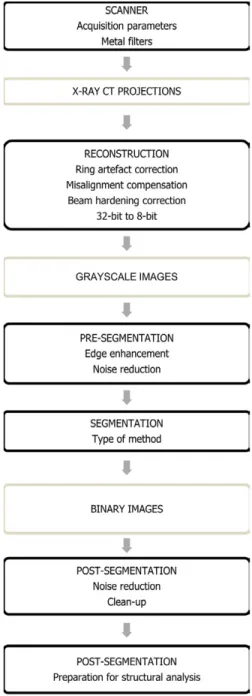
pore network (Vogel et al., 2005) have also been conducted. These analyses assumed that the pore space description generated from the image processing accurately represents the physical reality of the sample microstructure, but the choice of X-ray computed tomog-raphy (CT) image processing methodology has a visible impact on the resulting structure. Figure 1 shows an example of the processing steps from sample acquisition to binary image. Each step involves choosing the appropriate method and parameters, which are numer-ous and can have a profound effect on the resulting structure. These choices ultimately depend on the experience of the operator. What is important here is not only the diversity of these choices but
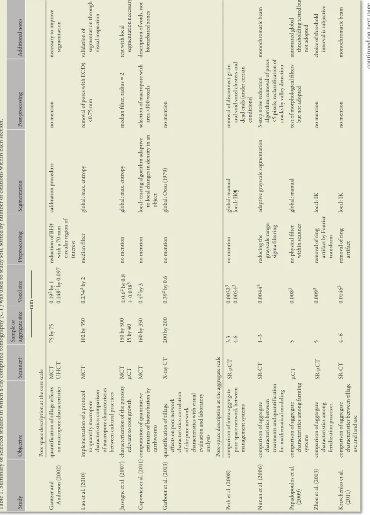
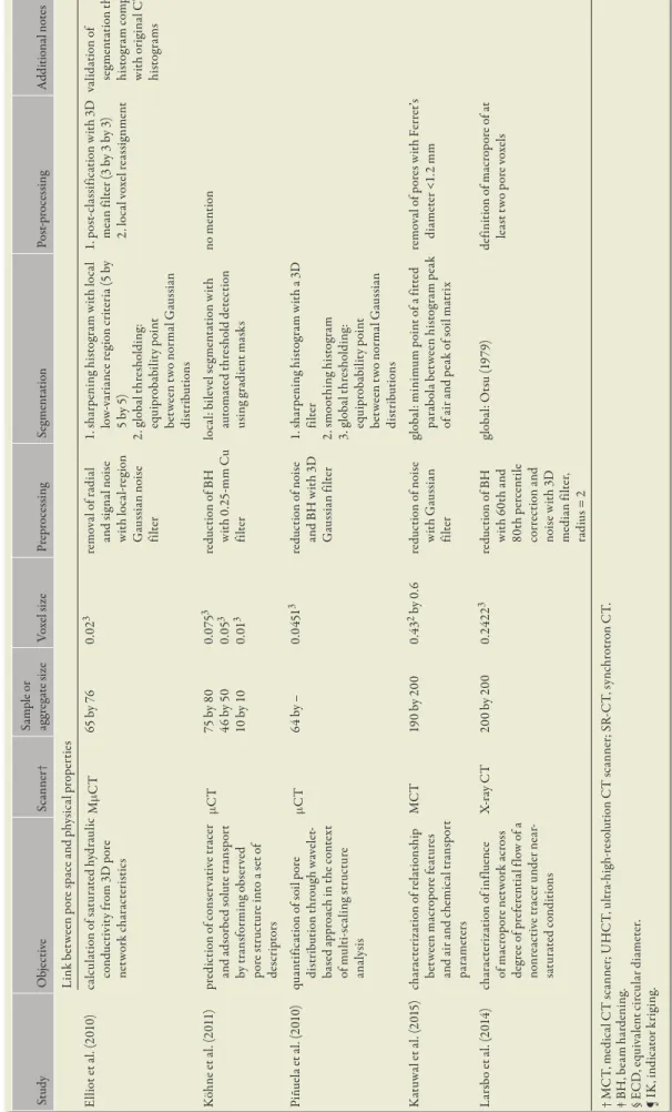
also the fact that they are often inadequately described or justified. Table 1 shows an example of the diversity of methodologies used in
a selection of soil science research papers (selection based on number of citations and diversity of research teams). Within Table 1, the pre-segmentation and post-segmentation steps are differentiated. Pre-segmentation steps are varied and are more efficient at handling image degradation than post-segmentation processing; a general rule (for more than just image analysis) is that the more upstream a problem is corrected, the easier is it to process the data downstream. Segmentation is the essential step when pixels are assigned to either the solid or porous phase. There are numerous segmentation meth-ods; a review of those used in soil science was provided by Tuller et al. (2013). In this study, we differentiated global and local thresh-olding methods. The aim of a threshthresh-olding method is to select a grayscale value, manually or automatically, that separates the image gray levels into two groups: greater than or equal to the threshold (TH) and less than the TH. In soil science, these two groups are often defined as the solid phase (soil matrix) and the void phase (pore space). With global thresholding, a constant TH is chosen for the entire image, whereas with local thresholding, the value is computed for every pixel based on the local neighborhood (Tuller et al., 2013). Segmentation precision depends on the initial quality of the grayscale images. Enhancing the projections before reconstruc-tion and the reconstructed images before segmentareconstruc-tion is the typical approach, but each research team has its own procedures (see Table 1). An efficient method for enhancing image quality is to apply noise reduction filters (Kaestner et al., 2008; Wildenschild and Sheppard, 2013) as mentioned in six of the 15 studies listed in Table 1. Some researchers have shown (Beckers et al., 2014b; Lamandé et al., 2013; Peth et al., 2008; Peng et al., 2014; Tarquis et al., 2009) that, in most practical cases, the choice of segmentation method plays a crucial role in the resulting pore structure, but no standards have yet been proposed. Several studies have sought to classify thresholding techniques based on information available from the resulting binary images (Baveye et al., 2010; Houston et al., 2013b; Iassonov et al., 2009; Schlüter al., 2014). So far as we know, only Wang et al. (2011) have used synthetic soil aggregate images, from which ground-truth information was available, to compare thresh-olding methods. Even these studies were based on image-by-image analyses and did not provide a tool with which to properly evaluate the processing methodologies.
Within this context, our study sought to provide a statistical analy-sis of the segmentation processing effects on the resulting data. By evaluating Otsu’s global method (Otsu, 1979), the local adaptive-window indicator kriging (IK) method (Houston et al., 2013a), and the porosity-based (PBA) global method (Beckers et al., 2014b) on two-dimensional simulated soil images from which ground-truth information was available, we could also objectively support existing reviews. The first objective of our study was to quantify the effects of pre-segmentation noise reduction on the accuracy of the thresh-olding method based on the performance indicators. The second objective was to evaluate the impact of post-segmentation process-ing on pore functionalities. The third objective was to propose an Fig. 1. Processing steps from sample to binary image. Some sources of
Ta bl e 1 . S um m ar y o f s el ec te d s tu di es i n w hi ch x -ra y c om pu te d t om og ra ph y ( C T ) w as u se d t o s tu dy s oi l, s or te d b y n um be r o f c ita tio ns w ith in e ac h s ec tio n. St ud y O bj ec tiv e Sc an ne r† Sa m pl e or ag gre ga te s iz e Vo xe l s iz e Pre pro ce ss in g Se gm en ta tion Pos t-p ro ce ss ing A dd ition al n ot es —————— m m —————— Po re s pa ce d es cr ip tion a t t he c ore s ca le G an tz er a nd A nd er son ( 20 02 ) qu an tif ic at ion o f t ill ag e e ff ec ts on m ac rop ore c ha ra ct er ist ic s MC T U HC T 75 b y 75 0. 19 2 by 1 0. 14 8 2 by 0 .0 97 re du ct ion o f B H ‡ w ith a 7 0-m m ci rc ul ar re gion o f int er es t ca lib ra tion p ro ce du re no m en tion ne ce ss ar y t o i m prov e se gm en ta tion Lu o e t a l. ( 20 10 ) im pl em en ta tion o f a p ro to co l to q ua nt ify m ac rop ore ch ar ac te ri st ic s; c om pa ri son of m ac rop ore c ha ra ct er ist ic s be tw ee n c ul tu ra l p ra ct ic es MC T 10 2 b y 3 50 0. 23 4 2 by 2 m edi an fi lte r glo ba l: m ax . e nt rop y re m ov al o f p ore s w ith E C D § <0 .75 m m va lid at ion o f se gm en ta tion t hro ug h vi su al ins pec tio n Ja ss og ne e t a l. ( 20 07 ) ch ar ac te ri za tion o f t he p oro sit y re le va nt t o ro ot g ro w th MC T mCT 15 0 b y 5 00 15 b y 4 0 ± 0. 6 2 by 0 .8 ± 0 .03 8 3 no m en tion glo ba l: m ax . e nt rop y m ed ia n f ilt er , r ad iu s = 2 te st w ith lo ca l se gm en ta tion ne ce ss ar y C ap ow ie z e t a l. ( 20 11 )c om pu ta tion o f q ua nt ita tiv e es tim at es o f b io tu rb at ion b y eart hw or m s MC T 16 0 b y 3 50 0.4 2 by 3 no m en tion lo ca l: t ra ci ng a lg or ith m a da pt iv e to lo ca l c ha ng es i n d en sit y i n a n obj ec t se le ct ion o f m ac rop ore w ith are a > 10 0 v ox el s de sc rip tion o f v oi ds , n ot bio tu rb at ed z one s G ar bo ut e t a l. ( 20 13 ) qu an tif ic at ion o f t ill ag e ef fe ct s on p ore ne tw or k ch ar ac te ri st ic s: c or re la tion of t he p ore ne tw or k ch ar ac te ri st ic s w ith v isu al ev al ua tion a nd l ab or at or y an al ysi s X -r ay C T 20 0 b y 2 00 0. 39 2 by 0 .6 no m en tion glo ba l: O ts u ( 19 79 ) no m en tion Po re -s pa ce d es cr ip tion a t t he a gg re ga te s ca le Pe th e t a l. ( 20 08 ) co m pa ri son o f i nt ra-ag gre ga te po re -s pa ce ne tw or k b et w ee n m an ag em en t s ys tem s SR-mCT 3.3 4.6 0. 00 32 3 0. 005 4 3 no m en tion glo ba l: m an ua l lo ca l: I K ¶ re m ov al o f d isc on ne ct g ra in and v oi d v ox el c lu st er s a nd de ad e nd s ( und er c er ta in cond ition s) N un an e t a l. ( 20 06 ) co m pa ri son o f a gg re ga te ch ar ac te ris tics be tw ee n tre at m en ts a nd q ua nt ifi ca tion fo r m at he m at ic al m ode lin g SR-C T 1–3 0.0 04 4 3 re du ci ng t he gr ay sc al e r an ge ; sig m a f ilt er in g ad ap tiv e g ray sc al e s eg m en ta tion 3-st ep n oi se re du ct ion al go rit hm ; re m ov al o f p ore s <5 p ix el s; re cl as sif ic at ion o f cr ac ks b y v al le y d et ec tion m on oc hro m at ic b ea m Pa pa dop ou lo s e t a l. (2 00 9) co m pa ri son o f a gg re ga te ch ar ac te ri st ic s a m on g f ar m in g sy st em s mCT 5 0.0 08 3 no p hy sic al f ilt er w ith in s ca nne r glo ba l: m an ua l te st o f m or pho lo gi ca l f ilt er s bu t n ot a dop te d au to m at ed g lo ba l th re sho ld in g t es te d b ut no t a dop te d Z ho u e t a l. ( 20 13 ) co m pa ri son o f a gg re ga te ch ar ac te ri st ic s a m on g fe rt ili za tion p ra ct ic es SR-mCT 5 0.0 09 3 re m ov al o f r in g ar tif ac t b y F ou rie r tr an sfo rm lo ca l: I K no m en tion cho ic e o f t hre sho ld in te rv al i s s ub je ct iv e K ra vc he nk o e t a l. (2 01 1) co m pa ri son o f a gg re ga te ch ar ac te ris tics be tw ee n t ill age us e a nd l and u se SR-C T 4– 6 0. 014 6 3 re m ov al o f r in g ar tifac t lo ca l: I K no m en tion m on oc hro m at ic b ea m co nt in ue d o n nex t p ag e
St ud y O bj ec tiv e Sc an ne r† Sa m pl e or ag gre ga te s iz e Vo xe l s iz e Pre pro ce ss in g Se gm en ta tion Pos t-p ro ce ss ing A dd ition al n ot es Li nk b et w ee n p ore s pa ce a nd p hy sic al p rop er tie s El lio t e t a l. ( 20 10 ) ca lc ul at ion o f s at ur at ed h yd ra ul ic cond uc tiv ity f ro m 3 D p ore ne tw or k c ha ra ct er ist ic s M mCT 65 b y 7 6 0. 02 3 re m ov al o f r ad ia l and s ig na l n oi se w ith lo ca l-re gion G au ss ia n n oi se filt er 1. s ha rp en in g h ist og ra m w ith lo ca l lo w -v ar ia nc e re gion c rit er ia ( 5 b y 5 b y 5 ) 2. g lo ba l t hre sho ld in g: eq ui pro ba bi lit y p oi nt be tw ee n t w o n or m al G au ss ia n di st rib ut ion s 1. p os t-c la ss ifi ca tion w ith 3 D m ea n f ilt er ( 3 b y 3 b y 3 ) 2. lo ca l v ox el re as sig nm en t va lid at ion o f se gm en ta tion t hro ug h hi st og ra m c om pa ri son w ith or ig in al C T hi sto gr am s K öh ne e t a l. ( 20 11 ) pre di ct ion o f c on se rv at iv e t ra ce r and a ds or be d s ol ut e t ra ns po rt by tr an sfo rm ing o bs er ve d po re s tr uc tu re i nt o a s et o f de sc rip to rs mCT 75 b y 8 0 46 b y 5 0 10 b y 10 0. 075 3 0. 05 3 0. 01 3 re du ct ion o f B H w ith 0 .2 5-m m C u filt er lo ca l: b ile ve l s eg m en ta tion w ith au to m at ed t hre sho ld d et ec tion us in g g ra di en t m as ks no m en tion Pi ñu el a e t a l. ( 20 10 ) qu an tif ic at ion o f s oi l p ore di st rib ut ion t hro ug h w av el et -ba se d a pp ro ac h i n t he c on te xt of m ul ti-sc al in g s tr uc tu re an al ysi s mCT 64 b y – 0. 04 51 3 re du ct ion o f n oi se and B H w ith 3 D G au ssi an fi lter 1. s ha rp en in g h ist og ra m w ith a 3 D filt er 2. sm oo thin g hi st og ra m 3. g lo ba l t hre sho ld in g: eq ui pro ba bi lit y p oi nt be tw ee n t w o n or m al G au ss ia n di st rib ut ion s K at uw al e t a l. ( 20 15 ) ch ar ac te ri za tion o f re la tion sh ip be tw ee n m ac rop ore f ea tu re s and a ir a nd c he m ic al t ra ns po rt pa ra m et er s MC T 19 0 b y 2 00 0.4 3 2 by 0 .6 re du ct ion o f n oi se w ith G au ss ia n filt er glo ba l: m in im um p oi nt o f a f itt ed pa ra bo la b et w ee n h ist og ra m p ea k of a ir a nd p ea k o f s oi l m at ri x re m ov al o f p ore s w ith F er re t’s di am et er < 1. 2 m m La rs bo e t a l. ( 20 14 ) ch ar ac te ri za tion o f i nf lu enc e of m ac rop ore ne tw or k a cro ss de gre e o f p re fe re nt ia l f lo w o f a non re ac tiv e t ra ce r u nd er ne ar -sa tu ra te d c ond ition s X -r ay C T 20 0 b y 2 00 0. 24 22 3 re du ct ion o f B H w ith 6 0t h a nd 80 th p er ce nt ile co rre ct ion a nd no ise w ith 3 D m edi an fi lte r, ra di us = 2 glo ba l: O ts u ( 19 79 ) de fin ition o f m ac rop ore o f a t le as t t w o p ore v ox el s † M C T, m ed ic al C T s ca nne r; U H C T, u ltr a-hi gh -re so lu tion C T s ca nne r; S R-C T, s ync hro tron C T. ‡ B H , b ea m h ar de ni ng . § E C D , e qu iv al en t c irc ul ar d ia m et er . ¶ I K , i nd ic at or k ri gi ng . Tab le 1. c on tin ue d.
approach for calculating the initial TH interval necessary using the local IK method based on the global TH calculated using the PBA method (Beckers et al., 2014b), considering that IK is sensitive to the initial choice of TH interval (Iassonov et al., 2009; Schlüter et al., 2010; Wang et al., 2011; Houston et al., 2013a).
6
Materials and Methods
Here we focus initially on the construction of our simulated images. The general framework was based on the methodology described
by Wang et al. (2011). It involved superimposing a realistic binary pore image (real soil [RS] images) on an image representing partial volume effects and then adding Gaussian noise (see Fig. 2 for a detailed illustration). We created 15 simulated images from the combination of 15 selected RS binary images and 15 generated par-tial volume effect images using a method based on fractals and the method of Wang et al. (2011). The thresholding methods tested should identify the pore region from the original RS image.
Real Soil Images
The RS images were derived from the Beckers et al. (2014a) study. We selected 15 two-dimensional images from silt loam soil. Details about the materials, sampling, and X-ray acquisition parameters can be found in Beckers et al. (2014a). Reconstructions were performed using NRecon software provided free of charge by Brucker micro-CT. This software provides tomographic artifact correction methods, which were not tested in this study. Automatic misalignment com-pensation was used, along with a Level 7 (out of 20) ring artifact correction. The RS images were not subjected to a beam hardening correction. In X-ray microtomography, the most commonly cited arti-fact is beam hardening due to the polychromatic nature of the X-ray beam, implying a deviation from the Beer Lambert law. For cylindri-cal objects, it results in a radial grayscylindri-cale intensity variation from the edges to the center. The beam hardening effect is barely distinguish-able from the circular compaction that occurs when sampling soil, and removing beam hardening effects might create noise. Finally, an intensity rescaling was applied to increase contrast (Tuller et al., 2013).
Partial Volume Effect Images
The partial volume effect images were generated through the overlay-ing of decreasoverlay-ing resolution images, as proposed by Wang et al. (2011). Our addition to Wang’s method was to produce decreasing resolution fractal images with a fractal dimension calculated from the RS images’ fractal dimension (Steps A and B). Those images were then combined to form one partial volume effect image (Step C).
Fractal Geometry
Fractal geometry states that a fractal object has comparable fea-tures at different scales and can be described by a so-called fractal dimension, D, which is power-law dependent (Mandelbrot, 1983):
( )
( )
log log 1 N D r = [1]where N is the constant number of transformed elements at each iteration and r is the ratio between the dimension of the parent element and the dimension of the transformed element.
Because power-law dependencies have been observed in soil science, researchers have applied fractal geometry to the study of soil behav-ior (Pachepsky et al., 2000). For example, Russell and Buzzi (2012) successfully derived a soil-water retention curve from the pore-size distribution fractal dimension of a silt loam soil. Many studies have reported that this concept provides a good description of the complexity of soil microstructure (e.g., Kravchenko et al., 2011).
The Fractal Generator: Steps A and B
We generated two-dimensional fractal images with a fractal gen-erator using the pore–solid fractal approach (Perrier et al., 1999), which works as follows. The first action is the division of an initia-tor into n2 elements. Within these elements, a proportion of x/n2
is allocated to pore pixels and a proportion of y/n2 is allocated to
solid pixels. The remaining pixels (z/n2) are available for the next
iteration, which involves their division by n. This is a recursive process. Equation [1] then becomes
( ) ( ) log log z D d n = + [2]
where d is the Euclidian dimension.
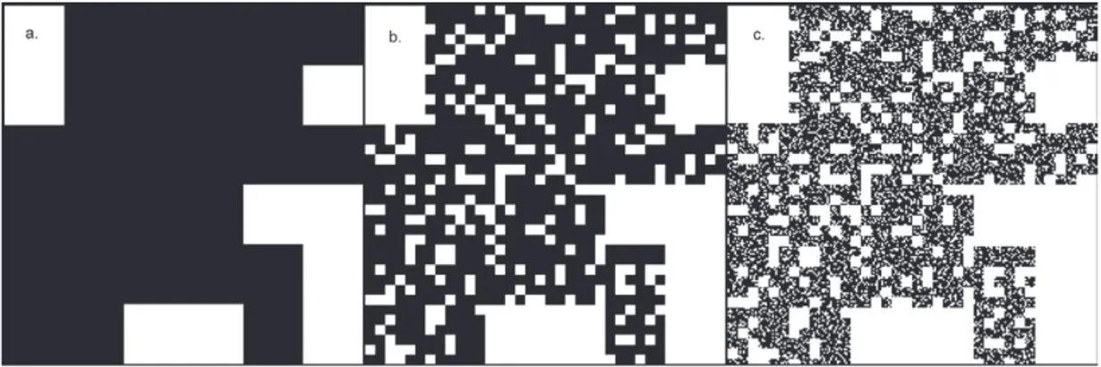
To construct partial volume effect images, we first generated decreas-ing resolution fractal images. This process was based on two main steps (A and B), each consisting of three fractal iterations. Step A involved generating fractal images to be used as the background of the final constructed partial volume effect image and represented by white pixels in Fig. 3c. These pixels could not be further modified during the rest of the process. Step B involved allocating smaller pixels to the solid and pore phases; the black pixels of Fig. 3c were the pixels subjected to further fractal divisions.
The fractal dimension in the Step A iterations was set as follows: 1. The fractal dimension of the associated RS image (Dobs in Table 2)
was calculated using the Fractal Box Counting tool available in the public domain image processing ImageJ (Version 1.47c, National Fig. 2. Detailed illustration of the simulated image construction.
Institutes of Health, http://rsb.info.nih.gov/ij). The number of diminishing size boxes containing pore pixels was counted. 2. The variable z of the RS image was calculated using Eq. [2] (zobs
in Table 2), considering that n = 6.
3. The variable z of the simulated image (zsim in Table 2) was cal-culated to represent the complement of zobs. It was calculated based on the fractal generator theory (see above), and therefore
2
obs sim sim sim
z =n -z =x +y [3]
4. The fractal dimension of the simulated image (Dsim in Table 2) was then calculated from zsim and n = 6 (Eq. [2]).
As noted above, Step B involved allocating smaller pixels to the solid and pore phases, and the black pixels in Fig. 3c are the pixels subjected to further fractal divisions. The three iterations of Step B (see Fig. 4) were produced with z = 2, n = 2, and D = 1:
ʶ n = 2 because those images were used to construct the partial volume effect within a 2 by 2 pixels averaging process (see below). ʶ z = 2 because this was the only way of having at least one pore pixel and one solid pixel with at least two elements remaining for the next step.
Partial Volume Effect Image Construction: Step C
The partial volume effect construction following the method of Wang et al. (2011) was applied to the generated fractal images (from Step B), and Fig. 4c shows the first image to be processed. From a size of 1728 by 1728, the image was scaled down into an 864 by 864 image by calculating the average of 2 by 2 squares. The down-scaled image (Fig. 4c) was then overlaid on Fig. 4b, which had also been down-scaled from 1728 by 1728 to 864 by 864, by adding the corresponding pixel color to fully represent the effect of all sizes of pores. This newly created image (not shown) was scaled down to 432 by 432 using the same averaging process, overlaid on Fig. 4a, and the resulting image was then scaled down to 216 by 216 by averaging. The result is shown in Fig. 5. Figure 6 illustrates the impact of the averaging process between Fig. 4c and Fig. 5.
Simulated Image Construction
The next step involved the overlaying of Fig. 5 on the correspond-ing RS image derived from Beckers et al. (2014a). We then added random normal noise to the pure white and pure black pixels, and variance and means were calculated from our scanner noise by scan-ning the empty chamber (within [0; 255]: mean = 222 and variance = 15.9). The final step was to add Gaussian noise (mean = 0; variance = 0.01) to the whole image to represent high-frequency noise (Fig. 7).
Pre-Segmentation Processing
Adhering to an algebraic comparison in its strictest sense, the effect of a pre-segmentation median filter (PRE0, none; PRE1, radius one pixel; PRE2, radius two pixels) was tested on the segmentation qual-ity of the simulated images. Median filters assign the median value of the neighboring pixels to the center pixel. These filters are less sensi-tive to extreme values and no grayscale value is created near the object boundary, resulting in the object edges being better preserved (Tuller Fig. 3. Step A in the generation of decreasing resolution fractal images for Image no. 1, sorted by iteration from left to right: construction of the partial volume effect background. The white pixels represent the soil matrix.
Table 2. Calculation of the fractal dimension (Dsim) for the simulated images, using the fractal dimension observed on the real soil image (Dobs), the observed number of fractals (zobs), and the simulated num-ber of fractals (zsim).
Image Dobs zobs zsim Dsim
1 1.20 9 27 1.85 2 1.43 13 23 1.75 3 1.53 15 21 1.69 4 1.52 15 21 1.70 5 1.21 9 27 1.84 6 1.30 10 26 1.81 7 1.14 8 28 1.86 8 1.72 22 14 1.48 9 1.31 10 26 1.81 10 1.38 12 24 1.78 11 1.61 18 18 1.62 12 1.58 17 19 1.65 13 1.61 18 18 1.61 14 1.48 14 22 1.72 15 1.45 13 23 1.74
et al., 2013). The use of a median filter before segmentation seems to be a common step in the field of soil X-ray CT image processing.
Tested Segmentation Methods
The complexity of segmentation is linked to the noise, artifacts, and partial volume effects in the grayscale images. Other sources of image degradation include ring artifacts, streak artifacts, high-frequency noise, scattered photons, and distortions (Baruchel et al., 2000). Therefore, besides enhancing image quality, choosing the right segmentation method is crucial.
Global Methods
The global thresholding method described by Otsu (Otsu, 1979) was tested because it provides acceptable results (Iassonov et al., 2009) and can be used in preference to the IK method where there are poorly distinguishable histogram peaks (Wang et al., 2011). Despite its non-reliability and the existence of more recent and more efficient methods, it is still a widely used method for soil images, probably because it is rapid and easy to use. It automati-cally chooses a TH based on the minimization of the intraclass variance between two intensity classes of pixels. In our study, it was performed with MATLAB R2015a (The MathWorks).
As we had ground-truth information available, the TH that should be applied could be estimated. Through an iterative loop, the TH
that minimized the difference between calculated porosity and ground-truth porosity was selected, and this value served as a bench-mark. This procedure was based on the method described by Beckers et al. (2014b). The MATLAB R2015a code was provided by the authors. Hereafter, we refer to the method as the PBA method.
Local Method
The IK method (Oh and Lindquist, 1999) has provided good results in various studies (Houston et al., 2013a, 2013b; Peth et al., 2008; Iassonov et al., 2009; Wang et al., 2011). Its variation, the adaptive-window indicator kriging method (Houston et al., 2013a), was chosen because Houston et al. (2013a) concluded that the adaptive method required fewer computational resources than the fixed one while providing very similar results. The IK concept relies on the selection of a TH interval, T1 to T2. All grayscale values below T1 are set at 0 and all values above T2 are set at 1. The values between T1 and T2 are assigned to a specific color, namely a phase, depend-ing on their grayscale value and their already classified neighbordepend-ing pixels. The adaptive-window IK method modifies this neighboring area based on locally available information to reduce the computa-tional costs when possible. The method was applied using the authors’ software, AWIK. The choice of T1 and T2 was based on edge detec-tion using the gradient masks (GM) method (Schlüter et al., 2010), an option available within AWIK software. Hereafter, we refer to the method as IK/GM.
Fig. 4. Step B in the generation of decreasing resolution fractal images for Image no. 1, sorted by iteration from left to right. The black pixels represent pores.
Fig. 5. Final partial volume effect constructed by the fractal generator for Image no. 1.
Fig. 6. The left-hand image is an enlargement of Fig. 4c (black rounded square in the upper right corner). The right-hand image is an enlarge-ment of a portion of Fig. 5 (black rounded square in the upper right corner).
Hybrid Method
The PBA method was shown to be satisfactory, although its perfor-mance was poorer than that of IK/GM (Beckers et al., 2014b). The weakness in IK is the choice of the T1 to T2 interval. Schlüter et al. (2010) proposed an improved automatic TH interval selection method, although it remained sensitive to noise. We therefore sought to combine the physical robustness of the PBA method with the edge-preserving IK method. The aim was to select a TH interval based on the global PBA threshold and then compute the IK method. The TH intervals tested were ±10, ±20, ±30, ±40, and ±50% of the global TH value. For example, if the PBA TH was 94 (on a 0–255 grayscale), the ±10% IK–PBA interval would be 85 to 103, the ±20% interval would be 75 to 113, and so on. Commonly, histogram percen-tiles would have been tested. We have, however, chosen this approach because the final objective would be to apply the IK–PBA to real soil images from which the porosity would be estimated with laboratory measurements. Because this porosity value would be uncertain, the global TH obtained with the original PBA method would also be uncertain. Therefore, the priority was that the interval include the supposedly “true” global TH value, corresponding to the “true” soil sample porosity. Hereafter, we will refer to the method as IK–PBA.
Post-Segmentation Processing
For a functional comparison, a post-segmentation median filter (POST0, none; POST2, radius two pixels) was also tested on the simulated images. A post-processing cleanup was also applied by removing the pores smaller than five pixels in area. The pore char-acterization was performed using the Analyze Particles tool that is available in the public domain image processing ImageJ (Version 1.47c, National Institutes of Health, http://rsb.info.nih.gov/ij).
6
Results Analysis
Performance Indicators
We used the ground-truth information available to compute the misclassification error (ME), whose value is between 0 and 1. It gives the proportion of pixels wrongly assigned to a phase. The
value 0 reflects perfect segmentation and the value 1 the opposite (Sezgin and Sankur, 2004):
0 T 0 T 0 0 ME 1 P P S S P S Ç + Ç = -+ [4]
where P0 is the number of pore pixels in the ground-truth image, PT is the number of pore pixels in the tested image, S0 is the number of solid pixels in the ground-truth image, and ST is the number of solid pixels in the tested image. We chose this simple indicator for its clear interpretation and because it offered the possibility of comparison with other studies (Wang et al., 2011; Schlüter et al., 2014).
Similarly, we used the relative error in the calculated porosity (RE_P) as a performance indicator. Calculated porosity is the ratio of black pixels (pores) to the total number of pixels.
Region non-uniformity (NU) was calculated to evaluate segmen-tation quality without using ground-truth information (Wang et al., 2011). High intra-region uniformity is achieved with a suitable segmentation method because there is a similarity of property in the region element; the variance in that property is then adequate for expressing the uniformity (Zhang, 1996):
2 p 2 NU P T s = s [5]
where P is the number of pore pixels, T is the total number of pixels, sp2 is the grayscale value variance in the pore pixels in the original
grayscale simulated image, and s2 is the total grayscale value
vari-ance in the original grayscale simulated image. Non-uniformity is a natural choice given the uniformity that a pore space should have, although it gives a poorer performance than the ground-truth information based indicator (Zhang, 1996).
Physical Performance
The physical evaluation of the segmentation methods was based on the pore network modeling concept, which is effective, for exam-ple, in computing soil-water retention curves (Vogel et al., 2005). Because we were dealing with two-dimensional images, we could focus only on the effects of segmentation on the two-dimensional pore network characteristics, such as pore geometry. More spe-cifically, we focused on the irregular pore shapes, which, despite their name, tend to be the norm rather than the exception in real soils. In addition to the empty–filled dynamic within pores, the wetting film plays an important role in fluid displacement (Celia et al., 1995). Irregular pore shapes have corners where there might be an accumulation of wetting fluid.
For each pore, we computed its shape factor as defined by Mason and Morrow (1991): 2 A G P = [6]
where A is the surface area (pixel2) and P is the perimeter (pixel).
Depending on the G value, we calculated the specific dimension-less conductance of each pore (Patzek and Silin (2001) (see Table 3). The dimensionless conductance g multiplied by the squared cross-section surface area (A2) and divided by the fluid viscosity
(m), gives the conductance g (L5 T M−1): 2
gA
g =m [7]
The volumetric flow rate through one pore was obtained by multi-plying the conductance (g) by the fluid displacement driving force. As in an electric circuit, where resistances are summed in series, con-ductance values were summed in parallel. We therefore multiplied each pore’s dimensionless conductance (g) by its squared surface area (A2) to sum all the conductance values (g) for each image, which
resulted in a global conductance value. The relative error in conduc-tance (RE_K) was calculated for each image. We also calculated the dimensionless conductance (g) relative error of each pore (RE_g). For the physical analysis, we then had two types of parameters: RE_K, reflecting the global conductance of the image, and RE_g, describing the pore shape accuracy. The RE_K and RE_g indica-tors were studied as absolute values.
Statistical Analysis
To assess whether or not the quality of the segmentation methods was altered by noise reduction, a three-way ANOVA was conducted to test for significant differences in the ME, NU, RE_P, and RE_K indicators for the various levels of noise reduction and the three segmentation methods. A randomized complete block design was applied, the simulated images being the random blocks. For the sig-nificant fixed interaction, three two-way ANOVAs were conducted (one per segmentation method) to test for a significant impact of noise reduction on the segmentation results. Tukey’s post-hoc test was performed in cases of a significant effect (p < 0.05).
To determine which segmentation method and noise reduction combination performed most accurately and to see if the IK– PBA method brought improvement, four two-way ANOVAs were conducted to test for significant differences in the ME, NU, RE_P, and RE_K values between the segmentation method and noise reduction combinations (10 levels). In cases of significance (p < 0.05), a post-hoc Dunnett test was conducted, with IK–PBA as the control.
In each case, similar analyses of RE_g were conducted. Because each pore had its own shape factor, each one of the 229 pores (for all 15 images combined) was considered as a random block.
6
Results and Discussion
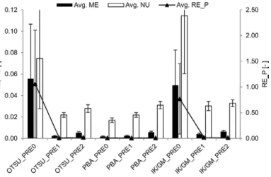
From a Structural Analysis
Figure 8 shows the ME, NU, and RE_P averaged for the 15 simu-lated images. With OTSU and IK/GM, PRE1 noise reduction filtering improved the segmentation accuracy because a decrease in indicator value meant an increase in segmentation accuracy. Compared with the results obtained by Hapca et al. (2013), Wang et al. (2011), and Schlüter et al. (2014), the ME and NU values for PRE1 and PRE2 were satisfactory. Without noise reduc-tion (PRE0), the ME value for OTSU was 60% lower than that obtained by Schlüter et al. (2014) but 34% higher for IK/GM. These high differences probably arose because we considered
aver-aged ME values with high standard errors. The OTSU_PRE0 and IK/GM_PRE0 performed very well for some images but poorly for others, with some porosity relative error values about 315% for OTSU and 500% for IK/GM. The PBA method performed well, with ME indicators below 0.01 and NU indicators below 0.05. In this case, where the exact porosity to reach was known, noise reduc-tion did not improve the PBA method. This is consistent with the working principle of PBA and with our experimental conditions. The segmentation was not perfect, however, highlighting the main
disadvantage of the selection of one threshold value for an entire two- (or three-) dimensional image.
Table 4 presents the relative variations in performance indicator values between two noise reduction levels for each segmentation method. First, the variations among the indicators were not com-parable. Therefore, to characterize the effect of one noise reduction,
Table 3. Dimensionless conductance (g) calculation depending on shape factor values (G) (Patzek and Silin, 2001).
G value Associated shape Conductance
G > 1/16 circle g » (3/5)G
(31/2)/36 < G < 1/16 square
g » 0.5236G
G < (31/2)/36 triangle
g » (1/2)G
Fig. 8. Averaged misclassification error (ME), region non-uniformity (NU), and porosity relative error (RE_P) for all segmentation methods (OTSU, porosity-based [PBA], and adaptive indicator kriging + gradient masks [IK/GM]) and for all pre-segmentation noise reductions (PRE0, PRE1, and PRE2).
it is advisable to use multiple and various performance indicators. Then, the variations from a PRE1 to a PRE2 noise reduction were
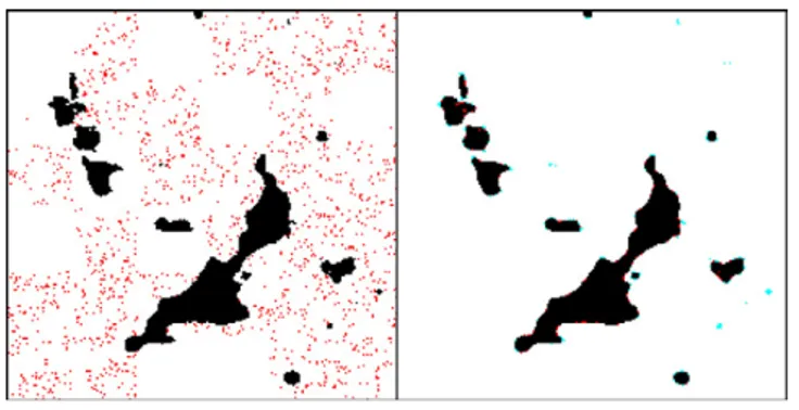
greater for the global segmentation methods (OTSU and PBA) than for the local IK/GM method albeit the histogram bimodal-ity was sharpened. This is, however, consistent with the study of Houston et al. (2013b), who found that OTSU gave a greater mean difference between two noise reduction levels than IK. Figure 9 shows the resulting images after OTSU and IK/GM segmentation for both noise reduction levels. Black pixels represent the pores that match the ground-truth information, the blue pixels represent pixels that are allocated to the soil matrix but should have been allocated to pores, and the red pixels are those allocated to pores but shouldn’t have been. With OTSU, from PRE1 to PRE2, small features are removed (blue pixels) and bigger pores have growing edges (red pixels). The differences between PRE1 and PRE2 for IK/GM are less striking.
With regard to the occurrence of the lowest ME, PBA_PRE0 provided the lowest indicator 12 times; together, PBA_PRE1 and OTSU_PRE1 provided the lowest one three times and almost always had the same ME value (13 times out of 15). In terms of NU, PBA_PRE0 always provided the lowest indicator value and, if its performance had not been taken into account, OTSU_PRE1 would always have provided the lowest ME and NU values. With regard to RE_P, OTSU_PRE1 and PBA_PRE1 provided the identical clos-est value to real porosity for 13 images. The IK/GM_PRE1 twice provided the lowest RE_P. This is not consistent with the findings reported by Wang et al. (2011), who concluded that IK performed better than OTSU in the case of clear bimodal histograms, which was the case with the simulated images. The difference between the two studies was probably due to the TH interval choice when using IK. The gradient masks method (Schlüter et al., 2010) for calculat-ing the TH interval was developed for unimodal images. We discuss this point further below. At no point did OTSU_PRE2 or IK/ GM_PRE2 give the best performance. Because the added noise on our simulated images is uncorrelated, PRE2 noise reduction seems to be disproportionate and destroys true information.
Statistical analyses confirmed that the PRE1 filter significantly improved segmentation accuracy with OTSU and IK/GM in terms of ME. With regard to NU, there was a significant difference between the three OTSU values (PRE0–PRE1–PRE2), but post-Tukey’s test was not able to determine the source of the difference. Similarly, PRE0 to PRE1 and PRE0 to PRE2 were significantly different for IK/GM, but in contrast RE_P significantly differen-tiated PRE0 to PRE1 and PRE0 to PRE2 for OTSU but not for IK/GM. These contrasting results illustrate the variability in indi-cator definitions and reflect the working principles of the global and local methods. The OTSU method gives different porosities by identifying porosity within the soil matrix where grayscale values are low (porosity is represented by black pixels). This leads to porosity without physical meaning, as noted by Hapca et al. (2013). The IK/GM method identifies the right pore region, but the limits might not be accurate. Therefore, despite a high gray-scale value, some pixels were taken into account, which increased the grayscale value variance and subsequently the NU. Wang et al. (2011) concluded that the use of NU is not enough for character-izing segmentation quality but provided acceptable results in the absence of ground-truth information. They observed that selecting the best segmentation method based on both ME and NU agreed for most images. Again, the use of multiple indicators allowed us to better characterize the accuracy of the segmentation methods. From ME, NU, and RE_P analyses and according to the experi-mental conditions, we showed that OTSU and IK/GM were more accurate with a PRE1 noise reduction and that OTSU_PRE1 and IK/GM_PRE1 were not statistically different.
Table 4. Misclassification error (ME), region non-uniformity (NU), porosity relative error (RE_P), and conductance relative error (RE_K) relative variations among the noise reductions (PRE0, PRE1, and PRE2) for the segmentation methods (Otsu, 1979 [OTSU], porosity-based [PBA], and adaptive indicator kriging + gradient masks [IK/ GM]).
Processing Relative variations
Noise reduction Segmentation ME NU RE_P RE_K
————————— % —————————
From PRE0 to PRE1 OTSU −96 −71 −99 −49
PBA 39 29 −14 152
IK/GM −92 −74 −97 −20
From PRE1 to PRE2 OTSU 131 27 132 66
PBA 129 42 28 80
IK/GM 62 8 −29 28
Fig. 9. Resulting Image no. 10 after the OTSU and the adaptive indi-cator kriging + gradient masks (IK/GM) segmentation methods for two level of pre-segmentation noise reduction (PRE1, PRE2). Black pixels represent the pores that match the ground-truth information, the blue pixels represent pixels that are allocated to soil matrix but should have been allocated to pore and the red pixels are the one allo-cated to pore but shouldn’t have been.
From a Functional Analysis
With regard to the global conductance results (RE_K), Fig. 10 depicts the averaged relative error for RE_K for all 15 images. Post-segmentation noise reduction always provided higher aver-aged RE_K with high standard errors. Indeed, post-segmentation noise reduction alters the pores edges and has influenced the pore conductance values (Fig. 11). However, post-segmentation has the advantage of removing small features wrongly assigned to porosity, albeit a post-segmentation cleanup could also do the job if those features are small enough.
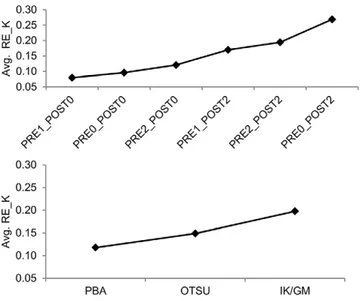
Table 5 presents the variations in RE_K between OTSU or IK/ GM and PBA. As noted above, PBA is here based on the images’ ground-truth information and should therefore perform well. The two global methods performed in a similar way when a PRE1 noise reduction was applied (low relative variations), which is consistent with previously discussed results. In this case, where we compared one segmentation method to a supposedly accurate segmentation method (PBA), the relative variations of RE_K were fairly similar to NU values. This is an interesting point because the NU indica-tor is calculated without ground-truth information, while RE_K is. The statistical analyses concluded that the segmentation method and combination of noise reduction factors separately had a significant impact on RE_K. Figure 12 shows the main factor effect plot for these factors. It shows that applying a post-segmentation noise reduction without any pre-segmentation noise reduction (combination PRE0– POST2) led to a significantly higher averaged relative error when compared with any combination of pre-segmentation noise reduction (PRE0–PRE1–PRE2) without post-segmentation noise reduction (POST0). In particular, a Tukey post-hoc test concluded that the com-parison of PRE0–POST0 (or PRE1–POST0) and PRE0–POST2 was highly significant (p < 0.01), and the comparison between PRE2– POST0 and PRE0–POST2 was significant (p < 0.05). Post-hoc tests also concluded that there was a significant difference between the
PBA and IK/GM methods but none between OTSU and IK/GM or between OTSU and PBA, as also illustrated in Fig. 13.
Figure 14 shows the tendency between noise reduction levels and segmentation methods with regard to RE_g (the relative error across the shape factor). We did not compute the PRE0 results because some pores had merged with OTSU and IK/GM and relative errors would increase without meaning. The OTSU and PBA methods had almost the same mean. This is consistent with the fact that global TH variation would lead to porosity variation within the soil matrix but less so around the pore region edges (also illustrated in Fig. 13). Post-segmentation noise reduction led to higher relative errors, which was consistent with the RE_K results. Some small pores were removed and pore edges were smoothed when POST2 was applied. There was no significant difference, however, among segmentation methods or the noise reduction levels, which was in contrast with the statistical results of RE_K.
Fig. 10. Averaged conductance relative error (RE_K) for all segmen-tation methods (Otsu, 1979 [OTSU], porosity-based [PBA], and adaptive indicator kriging + gradient masks [IK/GM]), for all pre-segmentation noise reductions (PRE0, PRE1, and PRE2), and for both post-segmentation noise reductions (POST0 and POST2).
Fig. 11. Resulting Image no. 6 after the OTSU (Otsu, 1979) seg-mentation method. The left-hand image was obtained without a pre- or post-segmentation noise reduction. The right-hand image was obtained without a pre-segmentation noise reduction and with a two-level post-segmentation noise reduction. Black pixels represent the pores that match the ground-truth information, the blue pixels rep-resent pixels that are allocated to the soil matrix but should have been allocated to pores, and the red pixels are those allocated to pores but shouldn’t have been.
Table 5. Misclassification error (ME), non-region uniformity (NU), porosity relative error (RE_P), and conductance relative error (RE_K) variations among the segmentation methods (Otsu, 1979 [OTSU], porosity-based [PBA], and adaptive indicator kriging + gradient masks [IK/GM]) for an identical pre-segmentation noise reduction (PRE0, PRE1, or PRE2).
Processing Relative variations
Segmentation Noise reduction ME NU RE_P RE_K ———————— % ————————
From OTSU to PBA PRE0 −97 −77 −99 −79
PRE1 8 0 −16 2
PRE2 7 11 −54 11
From IK/GM to PBA PRE0 −96 −85 −99 −83
PRE1 −38 −28 −64 −45
From a Threshold Analysis
Table 6 shows the TH median values for the segmentation meth-ods and associated noise reduction. For IK/GM, the TH interval boundaries tended to decrease from PRE0 to PRE1 and PRE2. For OTSU, this was also the case from PRE0 to PRE1. The TH then
increased, however, from PRE1 to PRE2. There was indeed a right-hand shift in the lower part of the soil matrix peak (see Fig. 15). At noise reduction PRE1, OTSU and PBA even had an identical TH. This could therefore be seen as a satisfactory noise reduction for the global method. As noted above, IK/GM performed better with pre-segmentation noise reduction. In those cases, the TH interval included the global TH from OTSU and PBA. With increasing noise reduction, the IK/GM TH interval increased. The TH2 was selected as the pore–solid boundary intensity level, and this one moved to a lower value with noise reduction (see Fig. 15). The TH1 selection was based on the TH2 value and the mode value. On the basis of these findings, we investigated the choice of a TH interval around the global TH computed by PBA.
Testing the Relevance of the IK–PBA Method
The IK–PBA method tended to combine the precision of the local IK method with the robustness of the global PBA method by select-ing the initial local TH interval around the global TH calculated by PBA. To perform a sensitivity analysis of the TH interval impact on the IK method, the TH interval around the global TH selected with Fig. 12. Main effect plots for the conductance relative error (RE_K).
The upper graph displays the pre-segmentation (PRE0, PRE1, and PRE2) and post-segmentation (POST0 and POST2) noise reduction combinations as variables. The lower graph displays the segmentation methods (porosity-based [PBA]; Otsu, 1979 [OTSU]; and adaptive indicator kriging + gradient masks [IK/GM]) as variables.
Fig. 13. Image no. 10 at various steps: (a) simulated image; (b) image after a PRE0 pre-segmentation noise reduction and OTSU segmen-tation (Otsu, 1979); (c) image after a PRE0 pre-segmensegmen-tation noise reduction and the porosity-based segmentation (PBA); and (d) image after a PRE0 pre-segmentation noise reduction and the adaptive indi-cator kriging + gradient masks segmentation (IK/GM).
Fig. 14. Main effect plots for the shape factor relative error (RE_g). The upper graph displays the pre-segmentation (PRE0, PRE1, and PRE2) and post-segmentation (POST0 and POST2) noise reduction combinations as variables. The lower graph displays the segmentation methods (porosity-based [PBA]; Otsu, 1979 [OTSU]; and adaptive indicator kriging + gradient masks [IK/GM]) as variables.
Table 6. Median threshold values according to segmentation methods (Otsu, 1979 [OTSU], porosity-based [PBA], and adaptive indica-tor kriging + gradient masks [IK/GM]) and pre-segmentation noise reductions (PRE0, PRE1, and PRE2); TH1 and TH2 represent the threshold interval for the local method.
Noise reduction
Segmentation method
OTSU PBA IK/GM TH1 IK/GM TH2
PRE0 125 102 147 180
PRE1 121 121 114 162
PBA ranged from ±10 to ±50%. We found that the ME indicator remained unchanged for the intervals ±10, ±20, and ±30%. After that, ME increased constantly, reaching about 25% of the initial ME value at the ±50% interval. For the following operations, we present only the segmentation results with a ±10% TH interval. First, the averaged ME (0.0023), NU (0.0217), RE_P (0.0096), and RE_K (0.064) values for IK–PBA were all in the same range as those from PBA or OTSU_PRE1. For ME, IK–PBA had the best performance twice, but for NU, RE_P, or RE_K it never had the best perfor-mance. The statistical analyses confirmed this trend by showing only OTSU_PRE0 and IK/GM_PRE0 as significantly different from IK–PBA in terms of ME, NU, and RE_P. When including post-segmentation noise reduction, RE_K analyses showed that post-segmentation noise reduction did not produce a significantly different result with IK–PBA. The IK–PBA method provided a significant improvement, however, compared with IK/GM_PRE0_ POST2, which was consistent with previous findings. The RE_g again gave contrasting results. According to this indicator, IK–PBA gave the best results and differed significantly from any other com-bination of method and noise reduction. The IK–PBA method therefore produced the correct binary images without the use of a noise reduction process (as opposed to OTSU_PRE1) and without knowing the real characteristics of the RS image used to construct the simulated images (as opposed to PBA). This is consistent with
the recommendation made by Iassonov et al. (2009) and Iassonov and Tuller (2010) that a local method could be used as an alterna-tive to pre-segmentation processing. As noted above, the choice of the TH interval is of prime importance when using IK. With the two-peak histogram simulated image, the interval around the global PBA TH produced far better results than the interval calculated by the gradient masks method (Schlüter et al., 2010), and this made the original idea of IK–PBA attractive.
6
Conclusion
X-ray computed tomography is widely used in soil and hydrological sciences. To be able to apply it to many situations, the prior con-cern is to have an accurate and correct pore space description. This comes with suitable choices of image processing that will modify the information initially available on grayscale images. The conscious and relevant processing decisions are therefore of great importance. Within this context, various noise reduction and segmentation method combinations were tested on multiple simulated grayscale images to perform statistical analyses on five types of indicators. It was shown that pre-segmentation noise reduction through a median filter led to a significant improvement in segmentation accu-racy for the global segmentation method introduced by Otsu (1979) and for the local adaptive-window indicator kriging (Houston et al., 2013a) segmentation method whose threshold interval was calculated with the gradient masks method (Schlüter et al., 2010). Moreover, the statistical analyses did not significantly differentiate those two methods when a pre-segmentation median filter was applied. The PBA method calculated the global threshold value that
should be applied; however, the global segmentation wasn’t per-fect. Therefore, a pre-segmentation noise reduction filter seems to be a necessity with global thresholding. Post-segmentation noise reduction was shown to be detrimental to segmentation quality by altering the pore shapes.
The threshold interval choice with the IK method is of major importance. Adapting the calculating method to the type of image histogram is advised. Our approach (IK–PBA) based on the global threshold value calculated with the PBA method performed well by providing indicator values that were similar to those generated by PBA, but IK–PBA had the advantage of using neither ground-truth information nor noise reduction filters.
Acknowledgments
We acknowledge the support of the National Fund for Scientific Research (Brussels, Belgium). We also thank Dr. Alasdair Houston for providing the AWIK software and Professor Yves Brostaux for advising us on the statistical analyses. We thank the AgriGES project, its coordinator Professor Bernard Heinesh, and Donat Regaert for supplying the fractal generator code. Finally, we wish to thank the anonymous reviewers and the editor for improving the quality of this paper.
References
Baruchel, J., J.-Y. Buffière, E. Maire, P. Merle, and G. Peix. 2000. X-ray tomogra-phy in material science. Hermes Science Publ., Paris.
Fig. 15. Image no. 14 histograms with different pre-segmentation noise reductions. Top to bottom: PRE0, PRE1, and PRE2. The dotted line represents the global threshold obtained with the porosity-based (PBA) segmentation method; the plain bold line represents the upper threshold obtained with adaptive indicator kriging + gradient masks (IK/GM) segmentation.
Baveye, P.C., M. Laba, W. Otten, L. Bouckaert, P. Dello Sterpaio, R.R. Goswami, et al. 2010. Observer-dependent variability of the thresholding step in the quantitative analysis of soil images and X-ray microtomography data. Geo-derma 157:51–63. doi:10.1016/j.geoGeo-derma.2010.03.015
Beckers, E., E. Plougonven, N. Gigot, A. Léonard, C. Roisin, Y. Brostaux, and A. Degré. 2014a. Coupling X-ray microtomography and macroscopic soil measurements: A method to enhance near saturation functions? Hydrol. Earth Syst. Sci. 18:1805–1817. doi:10.5194/hess-18-1805-2014
Beckers, E., E. Plougonven, C. Roisin, S. Hapca, A. Léonard, and A. Degré. 2014b. X-ray microtomography: A porosity-based thresholding method to improve soil pore network characterization? Geoderma 219–220:145–154. doi:10.1016/j.geoderma.2014.01.004
Capowiez, Y., S. Sammartino, and E. Michel. 2011. Using X-ray tomography to quantify earthworm bioturbation non-destructively in repacked soil cores. Geoderma 162:124–131. doi:10.1016/j.geoderma.2011.01.011
Celia, M.A., P.C. Reeves, and L.A. Ferrand. 1995. Recent advances in pore scale models for multiphase flow in porous media. Rev. Geophys. 33:1049– 1057. doi:10.1029/95RG00248
Dal Ferro, N., A.G. Strozzi, C. Duwig, P. Delmas, P. Charrier, and F. Mora-ri. 2015. Application of smoothed particle hydrodynamics (SPH) and pore morphologic model to predict saturated water conductivity from X-ray CT imaging in a silty loam Cambisol. Geoderma 255-256:27–34. doi:10.1016/j.geoderma.2015.04.019
Elliot, T.R., W.D. Reynolds, and R.J. Heck. 2010. Use of existing pore models and X-ray computed tomography to predict saturated soil hydraulic conductiv-ity. Geoderma 156:133–142. doi:10.1016/j.geoderma.2010.02.010 Gantzer, C.J., and S.H. Anderson. 2002. Computed tomographic measurement
of macroporosity in chisel-disk and no-tillage seedbeds. Soil Tillage Res. 64:101–111. doi:10.1016/S0167-1987(01)00248-3
Garbout, A., L.J. Munkholm, and S.B. Hansen. 2013. Tillage effects on topsoil structural quality assessed using X-ray CT, soil cores and visual soil evalua-tion. Soil Tillage Res. 128:104–109. doi:10.1016/j.still.2012.11.003
Hapca, S.M., A.N. Houston, W. Otten, and P.C. Baveye. 2013. New local thresh-olding method for soil images by minimizing grayscale intra-class variance. Vadose Zone J. 12(3). doi:10.2136/vzj2012.0172
Helliwell, J.R., C.J. Sturrock, K.M. Grayling, S.R. Tracy, R.J. Flavel, I.M. Young, et al. 2013. Applications of X-ray computed tomography for examining biophysi-cal interactions and structural development in soil systems: A review. Eur. J. Soil Sci. 64:279–297. doi:10.1111/ejss.12028
Houston, A.N., W. Otten, P.C. Baveye, and S. Hapca. 2013a. Adaptive-window indicator kriging: A thresholding method for computed to-mography images of porous media. Comput. Geosci. 54:239–248. doi:10.1016/j.cageo.2012.11.016
Houston, A.N., S. Schmidt, A.M. Tarquis, W. Otten, P.C. Baveye, and S. Hapca. 2013b. Effect of scanning and image reconstruction settings in X-ray com-puted microtomography on quality and segmentation of 3D soil images. Geoderma 207-208:154–165. doi:10.1016/j.geoderma.2013.05.017 Iassonov, P., T. Gebrenegus, and M. Tuller. 2009. Segmentation of X-ray
com-puted tomography images of porous materials: A crucial step for charac-terization and quantitative analysis of pore structures. Water Resour. Res. 45:W09415. doi:10.1029/2009WR008087
Iassonov, P., and M. Tuller. 2010. Application of segmentation for correction of intensity bias in X-ray computed tomography images. Vadose Zone J. 9:187–191. doi:10.2136/vzj2009.0042
Jassogne, L., A. McNeill, and D. Chittleborough. 2007. 3D-visualization and anal-ysis of macro- and meso-porosity of the upper horizons of a sodic, texture-contrast soil. Eur. J. Soil Sci. 58:589–598. doi:10.1111/j.1365-2389.2006.00849.x Kaestner, A., E. Lehmann, and M. Stampanoni. 2008. Imaging and image
processing in porous media research. Adv. Water Resour. 31:1174–1187. doi:10.1016/j.advwatres.2008.01.022
Katuwal, S., T. Norgaard, P. Moldrup, M. Lamandé, D. Wildenschild, and L. de Jonge. 2015. Linking air and water transport in intact soils to macropore characteristics inferred from X-ray computed tomography. Geoderma 237–238:9–20. doi:10.1016/j.geoderma.2014.08.006
Köhne, J.M., S. Schlüter, and H.-J. Vogel. 2011. Predicting solute transport in structured soil using pore network models. Vadose Zone J. 10:1082–1096. doi:10.2136/vzj2010.0158
Kravchenko, A.N., A.N.W. Wang, A.J.M. Smucker, and M.L. Rivers. 2011. Long-term differences in tillage and land use affect intra-aggregate pore hetero-geneity. Soil Sci. Soc. Am. J. 75:1658–1666. doi:10.2136/sssaj2011.0096 Lamandé, M., D. Wildenschild, F.E. Berisso, A. Garbout, M. Marsh, P. Moldrup, et
al. 2013. X-ray CT and laboratory measurements on glacial till subsoil cores: Assessment of inherent and compaction-affected soil structure character-istics. Soil Sci. 178:359–368. doi:10.1097/SS.0b013e3182a79e1a
Landis, E.N., and D.T. Keane. 2010. X-ray microtomography. Mater. Charact. 61:1305–1316. doi:10.1016/j.matchar.2010.09.012
Larsbo, M., J. Koestel, and N. Jarvis. 2014. Relations between macropore net-work characteristics and the degree of preferential solute transport. Hydrol. Earth Syst. Sci. 18:5255–5269. doi:10.5194/hess-18-5255-2014
Luo, L., H. Lin, and S. Li. 2010. Quantification of 3-D soil macropore networks in different soil types and land uses using computed tomography. J. Hydrol. 393:53–64. doi:10.1016/j.jhydrol.2010.03.031
Mandelbrot, B.B. 1983. The fractal geometry of nature. W.H. Freeman and Co., San Francisco.
Mason, G., and N.R. Morrow. 1991. Capillary behavior of perfectly wetting liquid in irregular triangular tubes. J. Colloid Interface Sci. 141:262–274. doi:10.1016/0021-9797(91)90321-X
Nunan, N., K. Ritz, M. Rivers, D.S. Feeney, and I.M. Young. 2006. Investigating microbial micro-habitat structure using X-ray computed tomography. Geo-derma 133:398–407. doi:10.1016/j.geoGeo-derma.2005.08.004
Oh, W., and W.B. Lindquist. 1999. Image thresholding by indicator kriging. IEEE Trans. Pattern Anal. Mach. Intell. 21:590–602. doi:10.1109/34.777370 Otsu, N. 1979. A threshold selection method from gray-level histograms. IEEE
Trans. Syst. Man Cybern. 9:62–66. doi:10.1109/TSMC.1979.4310076 Pachepsky, Y.A., D. Giménez, J.W. Crawford, and W.J. Rawls. 2000.
Con-ventional and fractal geometry in soil science. In: Y.A. Pachepsky et al, editors, Fractals in soil science. Elsevier Science, Amsterdam. p. 7–18. doi:10.1016/S0166-2481(00)80003-3
Papadopoulos, A., N.R.A. Bird, A.P. Whitmore, and S.J. Mooney. 2009. Investi-gating the effects of organic and conventional management on soil ag-gregate stability using X-ray computed tomography. Eur. J. Soil Sci. 60:360– 368. doi:10.1111/j.1365-2389.2009.01126.x
Patzek, T.W., and D.B. Silin. 2001. Shape factor and hydraulic conductance in noncircular capillaries: I. One-phase creeping flow. J. Colloid Interface Sci. 236:295–304. doi:10.1006/jcis.2000.7413
Peng, S., F. Marone, and S. Dultz. 2014. Resolution effect in X-ray microcomput-ed tomography imaging and small pore’s contribution to permeability for a Berea sandstone. J. Hydrol. 510:403–411. doi:10.1016/j.jhydrol.2013.12.028 Perrier, E., N. Bird, and M. Rieu. 1999. Generalizing the fractal model of soil
structure: The pore–solid fractal approach. Geoderma 88:137–164. doi:10.1016/S0016-7061(98)00102-5
Peth, S., R. Horn, F. Beckmann, T. Donath, J. Fischer, and A.J.M. Smucker. 2008. Three-dimensional quantification of intra-aggregate pore-space features using synchrotron-radiation-based microtomography. Soil Sci. Soc. Am. J. 72:897–908. doi:10.2136/sssaj2007.0130
Piñuela, J., A. Alvarez, D. Andina, R.J. Heck, and A.M. Tarquis. 2010. Quantifying a soil pore distribution from 3D images: Multifractal spectrum through wave-let approach. Geoderma 155:203–210. doi:10.1016/j.geoderma.2009.07.007 Russell, A.R., and O. Buzzi. 2012. A fractal basis for soil-water
charac-teristics curves with hydraulic hysteresis. Geotechnique 62:269–274. doi:10.1680/geot.10.P.119
Schlüter, S., A. Sheppard, K. Brown, and D. Wildenschild. 2014. Image process-ing of multiphase images obtained via X-ray microtomography: A review. Water Resour. Res. 50:3615–3639. doi:10.1002/2014WR015256
Schlüter, S., U. Weller, and H.-J. Vogel. 2010. Segmentation of X-ray microto-mography images of soil using gradient masks. Comput. Geosci. 36:1246– 1251. doi:10.1016/j.cageo.2010.02.007
Sezgin, M., and B. Sankur. 2004. Survey over image thresholding techniques and quantitative performance evaluation. J. Electron. Imaging 13:146–165. doi:10.1117/1.1631315
Taina, I.A., R.J. Heck, and T.R. Elliot. 2008. Application of X-ray computed to-mography to soil science: A literature review. Can. J. Soil Sci. 88:1–19. doi:10.4141/CJSS06027
Tarquis, A.M., R.J. Heck, D. Andina, A. Alvarez, and J.M. Antón. 2009. Pore net-work complexity and thresholding of 3D soil images. Ecol. Complex. 6:230– 239. doi:10.1016/j.ecocom.2009.05.010
Tuller, M., R. Kulkarni, and W. Fink. 2013. Segmentation of X-ray CT data of po-rous materials: A review of global and locally adaptive algorithms. In: S.H. Anderson and J.W. Hopmans, editors, Soil–water–root processes: Advances in tomography and imaging. SSSA Spec. Publ. 61. SSSA, Madison, WI. p. 157–182. doi:10.2136/sssaspecpub61.c8
Vogel, H.-J., J. Tölke, V.P. Schulz, M. Krafczyk, and K. Roth. 2005. Comparison of a lattice–Boltzmann model, a full-morphology model, and a pore network model for determining capillary pressure–saturation relationship. Vadose Zone J. 4:380–388. doi:10.2136/vzj2004.0114
Wang, W., A.N. Kravchenko, A.J.M. Smucker, and M.L. Rivers. 2011. Com-parison of image segmentation methods in simulated 2D and 3D mi-crotomographic images of soil aggregates. Geoderma 162:231–241. doi:10.1016/j.geoderma.2011.01.006
Wildenschild, D., and A.P. Sheppard. 2013. X-ray imaging and analy-sis techniques for quantifying pore-scale structure and processes in subsurface porous medium systems. Adv. Water Resour. 51:217–246. doi:10.1016/j.advwatres.2012.07.018
Zhang, Y.J. 1996. A survey on evaluation methods for image segmentation. Pat-tern Recognit. 29:1335–1346. doi:10.1016/0031-3203(95)00169-7
Zhou, H., X. Peng, E. Perfect, T. Xiao, and G. Peng. 2013. Effects of organic and inorganic fertilization on soil aggregation in an Ultisol as characterized by synchrotron based X-ray micro-computed tomography. Geoderma 195– 196:23–30. doi:10.1016/j.geoderma.2012.11.003