Abiotic factors involved in predicting trace metal levels in freshwater bivalves

1.

INTRODUCTION.

ABIOTIC FACTORS INVOLVED IN

PREDICTING TRACE METAL LEVELS

IN FRESHWATER BIVALVES

A. Tessier and P.G.C. campbell

Industrialization has led to increasing fluxes of trace metals from terres trial and atmospheric

sources towards the aquatic environ ment. Mining operations and metal refining and processing

industries are important point sources of trace metals.

In

certain parts of the world (Eastern

Canada), atmospheric deposition also represents an important direct contribution of trace

metals to surface waters; the concomitant acidic de position may also lead to increased

mobilization ·of trace metals from terres trial sources to the aquatic system. As-a result of

complex physical, chemical and biological processes, most of the trace metals introduced into

the aquatic environment are found associated with the bottom sediments, where they constitute

a potential danger for benthic organisms.

Management of in-place contaminants is one of the major problems confronted by

governmental agencies responsible for the protection of the environ ment. In principle, remedial

actions such as reduction in waste disposal, chemical treatment of in-place contaminants,

capping or dredging can be undertaken; these actions are however costly.

It

is clear that the

development of rational, effective and economical strategies to solve the problem posed by

sediment-bound toxic metals will depend greatly on our ability to predict how remedial actions

will improve water quality and how these changed conditions will affect aquatic organisms.

Important progress in this direction will be made only by understanding the biogeochemical

processes governing metal accumulation by benthic organisms under field situations.

Abstract

We have developed and tested in the field a deterministic model to

predict metal accumulation in benthic organisms. In the formulation of

the model, we used concepts derived from the free-ion activity model

of metal-organism interactions and from surface complexation theory,

to relate metal concentrations in the organisms to those in the water

or in the surficial oxic sediments.

The model was successfully tested in the field for cadmium

accumulation in the freshwater bi valve

Anodonta grandis.

Linear

regression analysis indicated that Cd concentrations in the soft

tissues of the bivalve, [Cd(org)], are related to the free cadmium

concentrations, [Cd2

+],

estimated from the total dissolved Cd and

inorganic ligands concentrations: [Cd(org)]

=

44 [Cd2

+] +

10

(r2=0.81). In a further step, partitioning of cadmium between water

and surficial oxic sediments was interpreted, using surface

complexation concepts, in terms of sorption of this metal on two

sediment components: organic matter and iron oxyhydroxides. This

partitioning model relates the free Cd2

+ concentrations to sedimentary

variables (e.g:, total sedimentary Cd, iron oxyhydroxides and organic

carbon concentrations) and water pHi sedimentary variables can then be

model, based on well accepted theories, to predict metal accumulation in benthic organisms.

The idea behind this development was that such a model, because of its mechanistic basis,

should be of general applicability (i.e. it should apply to sites others than those used in the

model calibration). The specific objectives were: i) to derive predictive equations for trace metal

concentrations

in

bivalves that are valid for any aquatic environment where these organisms

can be found;

li)

to evaluate the utility of the bivalves as bioindicators for trace metals. By

coupling concepts from the free-ion model of trace metal organisms interactions with the

surface complexation theory, we have made substantial progress towards this general

objective, using Cd as our test metal.

2. MATERIAL AND METHODS.

2.1. Study area.

The sediments, associated porewater samples and bivalve specimens were collected at

littoral stations in lakes located

in

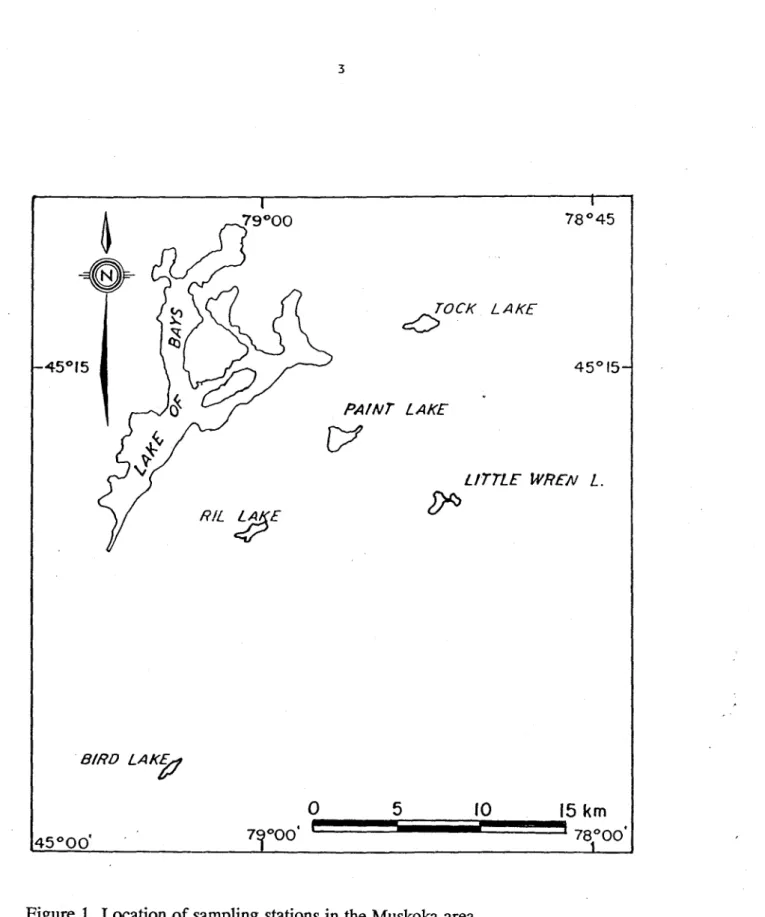
the Muskoka area, Ontario (Table 1; Figure 1). They lie on the

Precambrian Shield. The c10sest areas of industrial activities are Sudbury

200

km

northwest)

and Toronto

km

south).

2.2. Sampling.

The interstitial and overlying water samples were obtained with

in situ

samplers (porewater

peepers; 1 cm vertical resolution; 3 per lake) similar to those described by Hesslein (1976) and

Carignan

et al.

(1985). The peepers were filled with demineralized water and bubbled with

nitrogen for at least 24 h in plexiglass cylinders filled with demineralized water before being

inserted vertically in the lake sediments by a diver. After a two week equilibration period, the

peepers were retrieved from the sediments by a diver; samples were collected immediately

from five compartments above and five below the water-sediment interface, and pH was

measured in each sample (Carignan, 1984). Samples for dissolved sulfate and chloride analysis

were removed from the peepers with a syringe and injected into prewashed polypropylene

tubes; those for inorganic carbon determinations were obtained with a syringe and injected

through a septum into pre-evacuated and pre-washed glass tubes. The samples for the

PA/NT LAKE LITTLE WREN L. RIL ~E

!Y>

o

5

fO

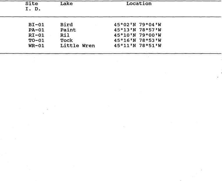
Table 1. Sample identification and location of .sampling stations in

the Muskoka area.

site

Bl-01

PA-01

Rl-01

TO-01

WR-01

Lake

Bird

paint

Ril

Tock

Little

Location

45°02'N 79°04'W

45°13'N 78°57'W

45°10'N 79°00'W

45°16'N 78°53'W

Wren

45°11'N 78°51'W

analysis of trace metals were collected by piercing the membrane (Gelman HT-2oo, 0.2

nominal pore size) with a Gilson pipette fitted with acid cleaned tips: these samples were

injected into pre-washed and pre-acidified (30 uL of IN Ultrex

HN0

final pH

<

2.5) Teflon

vials. Additional water was collected from the compartments 6 and 7 cm above the

sediment-water interface of each peeper (combined content 5 mL) for analysis, if necessary, by multiple

injection in flameless atomic absorption spectrophotometry (see below). On severa! occasions

during the summer, water samples were also collected by divers at many of the sites with a

clean polyethylene bottle close to the sediment-water interface for pH measurement. The

purpose of this measurement was to calculate time-averaged pH values (-log (L[H+]/n)) for the

summer period.

Sediment cores (4-5 per site) were collected by a diver, close to the peepers, with plexiglass

tubes (9 cm diameter). The tubes were tightly closed to minimize perturbations of the sediments

during their transport to the shore. The sediment cores were extruded on the shore, and only

the uppermost half centimeter, containing oxidized sediments, was retained. These samples

were placed in 500 mL centrifugation bottles half filled with lake water, and kept at ::::4

C during

transport to the laboratory where they were kept frozen until analysis.

Specimens of

Elliptio complanata

(10 per site) were obtained by a diver at each site, within a

radius of :::: 50 m from the sediment and porewater collection site. The bivalves were placed in

plastic bags with lakewater and maintained at:::: 4 oC during transport to the laboratory where

they were left to depurate for at least 24 h in aerated lake water. They were then dissected into

gills, mantle, hepatopancreas and remaining tissues, hereafter referred to as "remains". For

each sampling site, individual tissue types from the ten animals collected were pooled and

frozen at -20 oC until needed for analysis.

2.3 Analyses.

The water samples were analyzed for Cd, Cu, Ni, Pb, Zn, Fe, Mn,

S04' Cl, major cations and

organic and inorganic carbon. The metal concentrations were obtained by flame atomic

absorption spectrophotometry (AA) when possible (Fe, Mn, Ca, Mg, Na, K; Varian Techtron,

Model575ABQ or Model Spectra AA-20) or, otherwise, by flameless AA (Fe, Mn, Cd, Cu, Ni,

Pb, Zn; Varian Techtron, Model1275 or Spectra AA-30; GTA-95 or GTA-96). When initially

of five times the analytica1 detection limit (0.13 nmol L-I), its concentration was determined by a

multiple injection technique. The necessary number of aliquots were injected successively and

subjected to the preliminary drying steps; the combined sample was then atomized. The

detection limits for Ni and Pb were not improved with this technique. The National Research

Council of Canada (NRC) Riverine Water Reference Material (SLRS-2) was analysed for Cd, Cu

and Zn; we obtained 0.024+0.003

J1.g

Cd L-I (N=4; certified value 0.028+0.004

J1.g

Cd VI),

2.96+0.13

J1.g

Cu L-I (N =6; certified value 2.76+0.17

J1.g

L-I) and 3.38±0.07

J1.g

Zn L-l (N =7;

certified value 3.33+0.15

J1.g

L-l). The National Bureau of Standards Reference Materiall643b

(Trace Eleme~ts

in Water) was analyzed after lOX to 40X dilutions for Pb; we obtained:

25.7+2.4

J1.g

Pb L-l (N=4; certified value 24.1 +0.7

J1.g

Pb L-I). Sulfate and chloride

concentrations were determined by ion chromatography (Dionex Autolon, System 12);

dissolved inorganic carbon was measured by gas chromatography (Carignan 1984) and

dissolved organic carbon by persulfate-ultraviolet oxidation, followed by conductometric

determination of the released CO2 on a Technicon aûtoanalyser.

The surficial sediment samples were thawed and centrifuged to remove excess water;

subsamples (equivalent to

1 g dry wt.) were extracted and trace metals were partitioned into

the following empirica1 fractions (Tessier

et al.

1985): i) the sediment subsample was extracted

for 30 min with 1 N

ii) the residue from (i) was extracted for 5 h. with

adjusted to pH 5 with CH

COOH;

iii)

the residue from (ii) was extracted for 30 min. at room

temperature with 0.1 M

HCI in 0.1 N HN0

IV) the residue from (iii) was extracted for 6

h. at 96°C with 0.04 M

HCI in 25 % (v/v) CH

COOH; v) the residue from (iv) was

extracted for 5 h. at 85°C with

adjusted to pH 2 with HN0

and then at room temperature

with 3.2 M NH

0Ac in 20% (v/v) HN0

vi) the residue from (v) was digested successively with

concentrated HN0

(15 min; under reflux; followed by evaporation to dryness), concentrated

HCL0

(4 mL; 60 min under reflux) and HF (15 mL; evaporation to dryness; 12-18 h) and

dissolution of the residue was effected in 50 mL of 5 % HCL. Fe, Mn, Cd, Cu, Ni, Pb and Zn

concentrations in the extracts were determined by flame or flameless AAS, using the

appropriate extractant matrices for standards and blanks. Details of these procedures are given

in earlier publications (Tessier

et al.

1979, 1985). The National Research Council of Canada

reference sample of marine sediment MESS-l has been subjected to the sequential extraction

procedure. We measured, for the sum of the six fractions: 25.2+ 1.4 J..I.g Cu g-l (N=4; certified

value 25.1 +3.8 J..I.g Cu g-l), 169+2 J..I.g Zn g-l (N=4; certified value 191 + 17 J..I.g Zn g-l),

29.6+0.9 J..I.g Pb g-l (N=4; certified value 34.07-6.1 J..I.g Pb g-l). For Cd, and Ni"which showed

10wer than detection limit values in sorne fractions, we found the following

0.56+0.07

<

x

<

0.72+0.03 J..I.g Cd g-l (N=4; certified value 0.59+0.10 J..I.g Cd g-l) and

26.0+1.5

<

x

<

28.6+2.8 J..I.g Ni g-l (N=4; certified value 29.5+2.7 J..I.g Ni g-l). Sediment organic

carbon concentrations, {C

were determined with a CNS analyzer (Carlo-Erba, Model

NA15OO) after removal of inorganic carbon by acidification with diluted H

S0

(0.5 mol L-l; 15

min., 100

mL/g

sediment dry weight).

Bach pooled bivalve tissue was homogenized (Brinkman tissue grinder, Model CH-6010). A

subsample was then dried to constant weight to determine the wet:dry weight ratio, and a

second subsample was digested in a Teflon bomb with concentrated nitric acid (Aristar;

3 mL g-l of tissue dry weight) in a microwave oven at pressures between 5500 and 7000 KPa for

1 min. A certified reference material (lobster hepatopancreas, TORT-l, NRC) was submitted

to the same digestion procedure and analyzed for Cd, Cu, Ni, Pb and Zn; we obtained

24.1+0.5 J..I.g Cd g-l (N=5; certified value 26.3+2.1 J..I.g Cd g-l), 385+5 J..I.g Cu g-l (N=5; certified

value 439+22 J..I.g Cu g-l), 2.1 +0.3 J..I.g Ni g-l (N=4; certified value 2.3+0.3 J..I.g Ni g-l),

9.6+0.7 J..I.g Pb g-l (N=5; certified value 10.4+2.0 J..I.g Pb g-l) and 182+31 J..I.g Zn g-l (N=5;

certified value 177+ 10 J..I.g Zn g-l).

3.

RESULTS

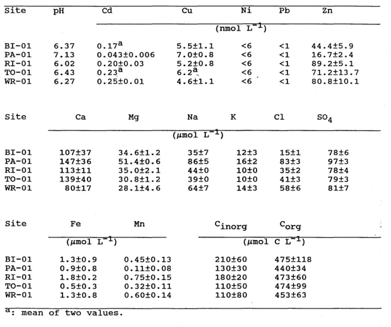
The concentrations of dissolved constituents above the sediment-water interface, as

obtained with the porewater peepers, are given in Table 2. Dissolved cadmium concentrations

vary between 0.04

0.25 nmol L-l; these values are much lower than those reported by

Hinch and Stephenson (1987) for Beech (3 nmol L-l) and Tock (3 nmol L-

_{Lakes. For this latter}

lake, we measured 0.23 nmol L-

_{Campbell and Evans (1991) measured values between 0.2}

and 1.25 nmol L-l in the epilimnia of various lakes in south-central Ontario; sorne of their

sampled lakes are in the Muskoka area. We measured dissolved Cu concentrations between

4.6 and 7.0 nmol L-

_{and Zn concentrations between 17 and 89 nmol L-l; these values are}

Table 2. Mean concentrations (±SD) of total dissolved constituents

(Ca, Cd, Cl, Cu, Fe, Mn, Ni, Pb, s04' Zn, pH, inorganic and organic

carbon) above the sediment-water interface, as obtained with the

porewater peepers.

site

pH

Cd

Cu

Ni

Pb

Zn

(runol L- 1 )

BI-01

6.37

0.17 a

5.5±1.1

<6

<1

44.4±5.9

PA-01

7.13

0.043±0.006

7.0±0.8

<6

<1

16.7±2.4

RI-01

6.02

0.20±0.03

5.2±0.8

<6

<1

89.2±5.1

TO-01

6.43

0.23a

<6

<1

71.2±13.7

WR-01

6.27

0.25±0.01

4.6±1.1

<6

<1

80.8±10.1

site

Ca

Mg

Na

Cl

S04

(l'mol

BI-01

107±37

34.6±1.2

35±7

12±3

15±1

78±6

PA-01

147±36

51.4±0.6

86±5

16±2

83±3

97±3

RI-01

113±11

35.0±2.1

44±0

10±0

35±2

78±4

TO-01

139±40

30.8±1.2

39±0

10±0

41±3

79±3

WR-01

80±17

28.1±4.6

64±7

14±3

58±6

81±7

site

Fe

Mn

_Cinorg

_Corg

(l'mol L 1)

(l'mol C L- 1 )

BI-01

1.3±0.9

0.45±0.13

210±60

475±118

PA-01

0.9±0.8

0.11±0.08

130±30

440±34

RI-01

1.8±0.2

0.75±0.15

180±20

473±60

TO-01

0.5±0.3

0.32±0.11

110±50

474±99

WR-01

1.3±0.8

0.60±0.14

110±80

453±63

slightly lower than those reported by Hinch and Stephenson (1987) for Beech (16 nmol Cu VI;

77 nmol Zn L-I) and Tock (16 nmol Cu L-I; 120 nmol Zn L-I) Lakes. The concentrations of

dissolved Ni and Pb were below our detection limits ( 6 and 1 nmol L-l respectively). For these

last two metals, multiple injections did not improve detection limits.

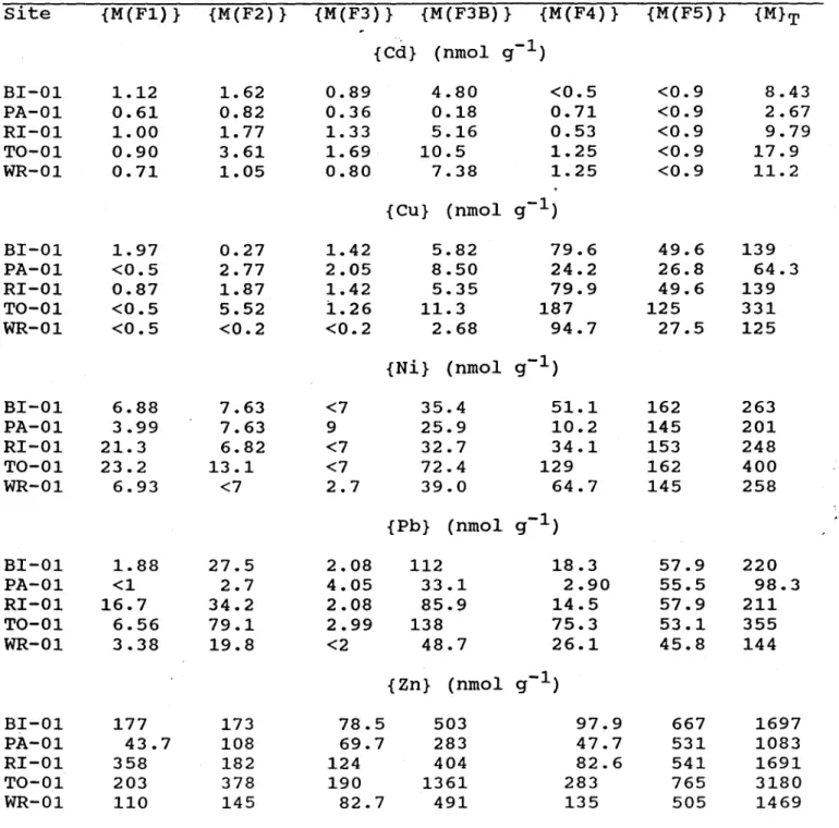
Concentrations of sedimentary trace metals obtained in various fractions vary slightly from

one lake to another (Table 3). Comparison of sediment trace metal concentrations among lakes

or with those obtained by other researchers is difficult, since the sediment samples were

obtained from the littoral zone of the lakes, where sediment composition is often patchy. The

. results show, however, general trends that were observed in other studies (Forstner and

Wittmann, 1981). For example, non-residual Cu is found mostly in fraction F4 (between 65%

(paint Lake) and 97% (Little Wren Lake», which confirms the high affinity of natural organic

matter for Cu. Large proportions of non-residual Pb (between 47% (Tock Lake) and 87% (Paint

Lake» and non-residual Zn (between 46%

(Ril

Lake) and 64% (paint Lake» are found in the

sum of fractions F3A and F3B; similar results were reported for suspended river sediments

(Tessier

et al., 1980). The ratio {COrg}:{Fe-ox} in the sediments ({Fe-ox} is the sum of

{Fe(F3A)} and {Fe(F3B)} in Table 3) varies between 10 (paint Lake) and 130 (Little Wren

Lake); this large variation in the ratio explains at least partIy variations in metal partitioning

observed among lakes. For example, the ratio [Cu(F4)]:([Cu(F3A)]

+

[Cu(F3B)]) is linearly

correlated (r2=0.92; N=5) with the ratio {COrg}:{Fe-ox}. This strong correlation suggests a

competition between iron oxyhydroxides and organic matter for copper; such a competition

has been reported by Luoma (1986).

Concentrations of Cd, Cu, Ni, Pb and Zn in the tissue of

E. complanata are given in Table 4. We ,

found that cadmium concentrations in the tissues of the bivalve varied between 13 and

26 J.1.g g-I. These values are similar to those reported for E. complanata by Servos et al., (1987)

for Lake of Bays (12

J.1.g g-l) and by Hinch and Stephenson (1987) for Beech (11 J.1.g g-l) and

Tock (15

J.1.g g-l) Lakes. The values obtained for Cu (between 5.9 and 7.3 J.1.g g-l) and Zn

(between 170 and 215

J.1.g g-l) are similar to those reported by Hinch and Stephenson (1987) for

Beech (7.3

J.1.g Cu g-l; 155 J.1.g Zn g-l) and Tock (10 J.1.g Cu g-l; 130 J.1.g Zn g-l) Lakes.

Table 3. Partitioning(*) of trace metals in the oxic layer of lake

sediments and concentration of sedimentary organic carbon. The

concentrations are given on a dry weight basis.

site

{M(F1)}

{M(F2)}

{M(F3)}

{M(F3B)}

{M(F4)}

{M(F5)}

{M}T

{Cd} (nmol g-l)

BI-01

1.12

1.62

0.89

4.80

<0.5

<0.9

8.43

PA-01

0.61

0.82

0.36

0.18

0.71

<0.9

2.67

RI-01

1.00

1. 77

1.33

5.16

0.53

<0.9

9.79

TO-01

0.90

3.61

1. 69

10.5

1.25

<0.9

17.9

WR-01

0.71

1.05

0.80

7.38

1.25

<0.9

11.2

{Cu} (nmol g-l)

BI-01

1.97

0.27

1.42

5.82

79.6

49.6

139

PA-01

<0.5

2.77

2.05

8.50

24.2

26.8

64.3

RI-01

0.87

1.87

1.42

5.35

79.9

49.6

139

TO-01

<0.5

5.52

1.26

11.3

187

125

331

WR-01

<0.5

<0.2

<0.2

2.68

94.7

27.5

125

{Ni} (nmol g-l)

BI-01

6.88

7.63

<7

35.4

51.1

162

263

PA-01

3.99

7.63

9

25.9

10.2

145

201

RI-01

21.3

6.82

<7

32.7

34.1

153

248

TO-01

23.2

13.1

<7

72.4

129

162

400

WR-01

6.93

<7

2.7

39.0

64.7

145

258

{Pb} (nmol g-l)

BI-01

1.88

27.5

2.08

112

18.3

57.9

220

PA-01

<1

2.7

4.05

33.1

2.90

55.5

98.3

RI-01

16.7

34.2

2.08

85.9

14.5

57.9

211

TO-01

6.56

79.1

2.99

138

75.3

53.1

355

WR-01

3.38

19.8

<2

48.7

26.1

45.8

144

{Zn} (nmol g-l)

BI-01

177

173

78.5

503

97.9

667

1697

PA-01

43.7

108

69.7

283

47.7

531

1083

RI-01

358

182

124

404

82.6

541

1691

TO-01

203

378

190

1361

283

765

3180

WR-01

110

145

82.7

491

135

505

1469

Table 3. (Continue).

site

{M(Fl)}

{M(F2)}

{M(F3)}

{M(F3B)}

{M(F4)}

{M(F5)}

{M}T

{Fe} (J,Lmol g-l)

BI-Ol

0.20

8.49

6.59

95.8

10.3

413

534

PA-Ol

0.20

4.03

6.52

105

3.65

397

517

RI-Ol

0.04

8.83

9.79

73.9

10.6

380

483

TO-Ol

0.06

6.79

7.07

113

33.9

544

705

WR-Ol

0.14

7.72

7.95

63.8

24.9

344

448

{Mn} (J,Lmol g-l)

BI-Ol

0.87

1.26

2.29

1.49

0.06

9.56

15.5

PA-Ol

0.55

2.02

25.3

3.08

0.06

9.65

40.7

RI-Ol

0.69

1.24

1.97

1.04

0.05

7.88

12.9

TO-Ol

0.88

1.48

0.87

1.18

0.05

6.19

10.7

WR-Ol

1.07

0.35

0.07

0.28

0.08

9.08

10.9

BI-Ol

4472

PA-Ol

1107

RI-Ol

3230

TO-Ol

9967

WR-Ol

9358

(*):

{M(Fl)} •.... {M(F5)} represent metal concentrations in fractions 1

to 6 following the sequence given in the texte

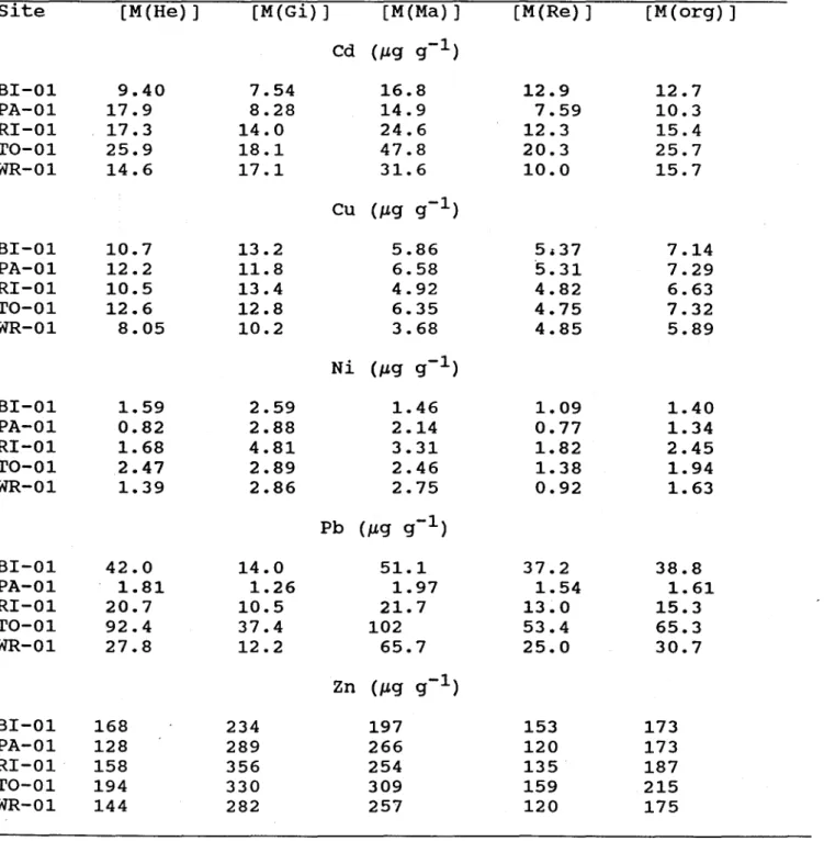
Table 4. Metal concentrations (on a

dry

weight basis) in the tissues of

Elliptio complanata

from

various sampling sites. He, hepatopancreas; Gi, gills; Ma, mantle; Re, remaining; org, whole

organisms.

site

[M(He}]

[M(Gi}]

[M(Ma)]

[M(Re}]

[M(org}]

Cd (J1.g g-l)

BI-01

9.40

7.54

16.8

12.9

12.7

PA-01

17.9

8.28

14.9

7.59

10.3

RI-01

17.3

14.0

24.6

12.3

15.4

TO-01

25.9

18.1

47.8

20.3

25.7

WR-01

14.6

17.1

31.6

10.0

15.7

Cu (J.Lg g-l)

BI-01

10.7

13.2

5.86

5.37

7.14

PA-01

12.2

11.8

6.58

5.31

7.29

RI-01

10.5

13.4

4.92

4.82

6.63

TO-01

12.6

12.8

6.35

4.75

7.32

WR-Ol

8.05

10.2

3.68

4.85

5.89

Ni (J1.g g-l)

BI-Ol

1.59

2.59

1.46

1.09

1.40

PA-Ol

0.82

2.88

2.14

0.77

1.34

RI-Ol

1.68

4.81

3.31

1.82

2.45

TO-Ol

2.47

2.89

2.46

1.38

1.94

WR-01

1.39

2.86

2.75

0.92

1.63

Pb (J1.g g-l)

BI-Ol

42.0

14.0

51.1

37.2

38.8

PA-Ol

1.81

1.26

1.97

1.54

1.61

RI-Ol

20.7

10.5

21.7

13.0

15.3

TO-Ol

92.4

37.4

102

53.4

65.3

WR-01

27.8

12.2

65.7

25.0

30.7

Zn

(J1.g

g-l)

BI-Ol

168

234

197

153

173

PA-01

128

289

266

120

173

RI-Ol

158

356

254

135

187

TO-01

194

330

309

159

215

WR-Ol

144

282

257

120

175

4. DISCUSSION

4.1 The free-ion activity mode!.

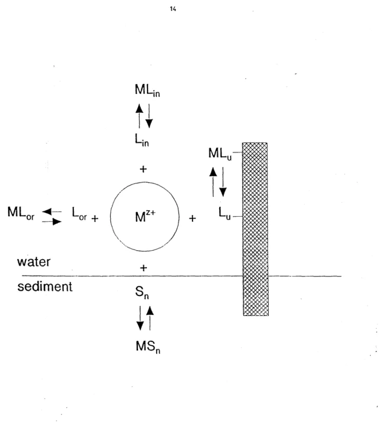
According to the free-ion activity model (Figure 2), the effects (including bioaccumulation) of

a trace metal M on an organism which obtains the trace metal from the water should be

predicted by the free ion concentration (or activity) of this metal, [Mz+]. The concentration of a

metal accumulated into an organism, [M(org)], should thus be written (Morel, 1983):

[M(org)]

=

f([M z

+])

where f means a function. This model has been developed for explaining (with great success)

biological effects of trace metals on unicellular organisms. Laboratory bioassays, conducted

with benthic animals exposed to dissolved metals under carefully controlled conditions, have

shown that the effects of trace metals on these animaIs are aIso related to the free metal ion

concentration and not to the total metal concentrations in the animaIs' environ ment. For

example, mortality of the shrimp

Palaemonetes pugio

exposed to cadmium was shown to be

related to [Cd2+] (Sunda

et al.,

1978). Similarly, short-term (14 d) accumulation of copper in the

American oyster

Crassostrea virginica

was found to be related to [Cu2+] (Zamuda and Sunda,

1982). Note, however, that the applicability of the free-ion activity model in the field, where

dissolved ligands (e.g. naturaI organic matter) differ from the synthetic ligands used in the

laboratory (e.g. NTA, EDTA), has never been demonstrated.

For the following discussion, we have focused on cadmium;

the metals measured,

water, sediment and animal data are more complete for this metal (other metals show many

"lower than detection limit" values, especially for the water samples). To enhance the

representativity of the study, we include aIso Cd data obtained for other lakes that we have

studied, which are located in the areas of Sudbury (On), Rouyn-Noranda (Qc; mining area;

heavily contaminated with Cd), Chibougamau (Qc; mining area), Québec (Qc) and Eastern

Townships (Qc). These lakes are distributed over a geographical area of about 350 000 km

and they represent a large gradient of Cd contamination and a wide range of pH vaIues. Since

additional measurements are needed to ob tain a satisfactory picture of Cd concentrations in

E.

+

MLor

~

Lor

+ (

MZ+

₊

water

+

sediment

Figure 2. Schematic representation of the various reactions occurring in the water overlying the

sediments. W+ is the free metal ion; L and L are dissolved inorganic and organic ligands

respectively;

L

is a ligand at the surface of an organism or a transport molecule; S is a

component of the sediment (e.g. iron oxyhydroxides; organic matter) which sorbs the trace

metal;

ML , ML ,ML and MS represent the metal bound to the various ligands or sediment

components.

discussion Cd data that we have obtained for another widespread freshwater bivalve,

Anodonta

grandis.

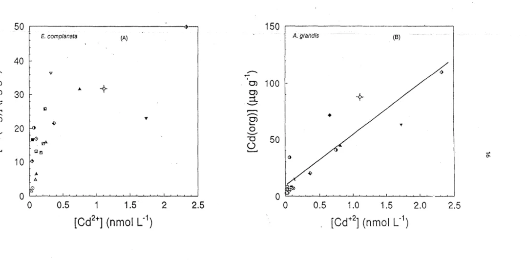
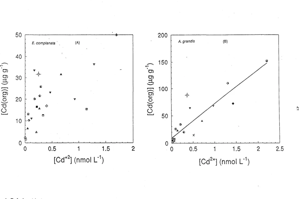
We have plotted in Figure 3 cadmium concentrations in

E.

complanata (Fig. 3a) and in A.

grandis

(Fig. 3b) as a function of [Cd

_{We have calculated [Cd}

_{with the equilibrium model}

HYDRAQL (papelis

et al., 1988), using the total dissolved Cd concentrations ([Cd]; Table 2),

the measured concentrations of the inorganic ligands concentrations (Table 2), and the stability

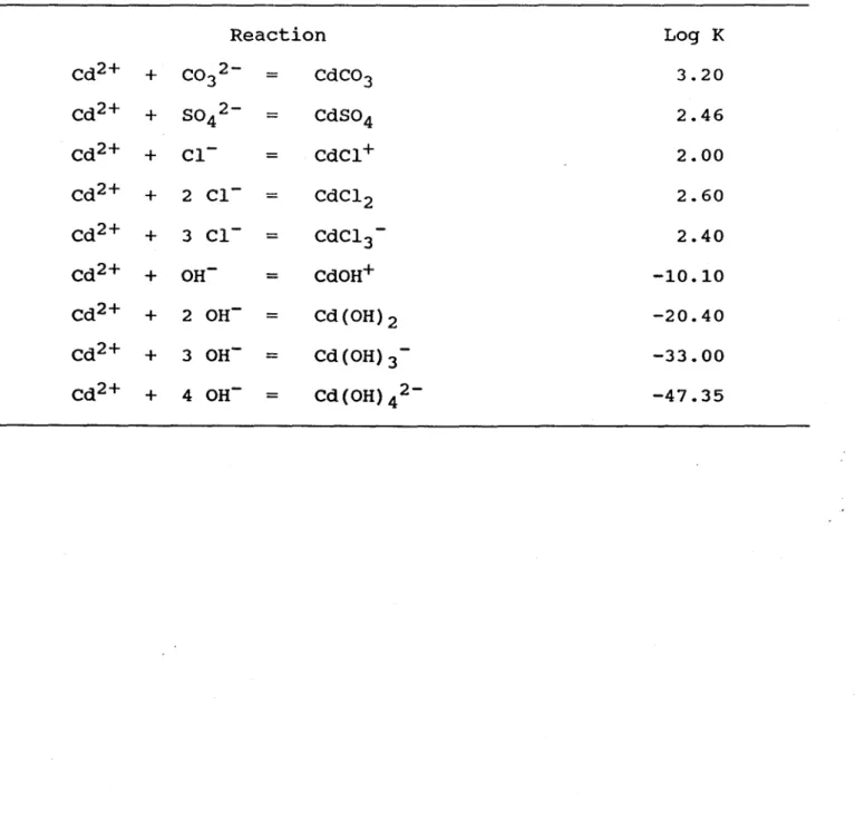
constants of the inorganic complexes (Smith and Martell, 1977); the stability constants used for

calculating Cd complexation are given in Table 5. Because the thermodynamic equilibrium

constants for Cd-DOM (dissolved organic matter) are unknown, possible cadmium

complexation by natural organic ligands could not be considered in the calculation.

According to the data in Figure 3b, Cd concentrations in the tissues of

grandis (J..Lg

g-l) can

be described by :

[Cd(org)]

=

44 (±5) [Cd2

+] +

10 (±15)

(n

=

17; r 2

=

0.81; [Cd2

+]

in nmol L-1 )

The relationship between cadmium concentration in

E. complanata and [Cd

_{is, however, not}

as clear; if data from D'Alembert Lake are removed, it would resemble an hyperbolic function.

Additional measurements, especially at sites where dissolved Cd concentrations are high, are

needed before a definitive interpretation can be made.

It

might be argued that much of the scatter in Figure 3a,b is due

variation in dissolved Cd

on short time sca1es (Tessier

et al., 1993). For example, Yan et al. (1990) reported a 2-fold

change in dissolved Cd concentration in Red Chalk Lake during the ice-free season; this lake is

located in the Muskoka area. Dissolved Cd concentrations used in the present study are mean

values for a single sampling. Cadmium concentrations in the bivalves are probably not sensitive

to short-term variations in dissolved Cd. For example, we have observed that Cd

concentrations in the tissues of

grandis

specimens transplanted from the unpolluted Lake

Brompton (Eastern townships) to the polluted Lake Joannes (Rouyn-Noranda area) had not

reached, after three years, the cadmium levels observed in the indigenous specimens from

Lake Joannes. The use of time-averaged values of dissolved Cd, instead of the single values

40

--..

--..

_,

100

+

::i.

30

+

::i.

---

--..

..,

20

---

---

₅₀

0

0

...

10

0

W

o

0

0.5

1

1.5

2

2.5

o

0.5

1.0

1.5

2.0

2.5

[Cd

+] (nmol L-

, [Cd+

(nmol L-

Figure 3. Relationship between cadmium concentration in the tissues (whole organisms) of

E. complanata

(A) or

A. grandis

. (B) and the free cadmium ion concentration calculated fram total dissolved Cd and inorganic ligands. Symbols represent

various sampling sites.

...

0-Table 5. stability constants used in the equilibrium model HYDRAQL

(Papelis et al., 1988) for the complexation with inorganic ligands.

Reaction

Log

Cd2 +

+

CO 2-

₃

₌

_CdC03

3.20

Cd2 +

+

SO 2-

₄

₌

_CdS04

2.46

Cd2+

+

CI-

CdCI+

2.00

Cd2 +

+

2 CI-

=

_{CdCl 2}

2.60

Cd2 +

+

3 CI-

_{CdCI 3-}

2.40

Cd2 +

+

OH-

CdOH+

-10.10

Cd2 +

+

2 OH-

Cd(OH)2

-20.40

Cd2 +

+

3 OH-

Cd (OH) 3

-

-33.00

Cd2 +

+

4 OH-

_{Cd(OH) 4 2-}

-47.35

function to predict cadmium concentration in

E. complanata

(Fig. 3a). Measurement of temporal

changes in Cd concentrations in the tissues of transplanted

grandis

specimens suggests

that they accumulate metals only during the warm season (e.g. from May to October). For

optimum predtctive power, the mean [Cd2+] should thus be preferentially obtained for this

period.

The data shown in Figure 3 are consistent with the free-ion activity model.

It

should be noted,

however, that very similar relations would have been obtained with total dissolved Cd ([Cd]),

since its concentration at all sites is close to the computed value for [Cd

Given the similarity

between [Cd

_{and [Cd] values, and the scatter shown in Fig. 3, it is not possible with the}

present data to demonstrate unambiguously that the free-ion activity model applies in the field

to Cd accumulation in

complanata

or

grandis.

To do so, one would need a natural setting

where the degree of complexation, a

=

[Cd]/[Cd2+], vary from site to site. Both

S04

and Cl are

known

complex Cd, but it is unlikely that

complanata

and

grandis

would

found in

freshwaters where these inorganic ligands are present in sufficiently high concentrations

complex Cd significantly.

An

alternative approach to demonstrate the application of the free-ion

activity model to Cd accumulation by the two bivalves in the field would

fmd sites where

natural organic matter complexes Cd significantly, provided of course that we can account for

this complexation and correctly estimate [Cd

4.2 Relationship between dissolved and surficial sedimentary Cd.

Cadmium concentrations in the surficial oxic sediments are related to dissolved Cd

concentrations in the overlying water, Le. in the bivalves' aqueous environment. The partitioning

of Cd between water and surficial oxic sediments has been interpreted, using surface

complexationconcepts, in terms of the sorption of this metal to the two following sediment

components: organic matter and iron oxyhydroxides. The development of this partitioning

model is discussed in detail in the paper by Tessier

et

al.,

(1993) given in the Appendix.

According to this partitioning model, [Cd

_{can be calculated from the following three}

[Cd2+]

{Fe-Cd} [H+]x

=

---*

NFe " KFe-Cd {Fe-ox}

(3a)

[Cd2+]

{OM-Cd} [H+]Y

=

---*

NOM" KOM-Cd {OM}

(3b)

(3e)

=

---*

+

y

*

+

x

NFe " KFe-Cd {Fe-ox} [H] + NOM" KOM-Cd {OM} [H ]

where:

- {Fe-ox} is the concentration of iron oxyhydroxides in the surficial sediments (nmol g-l)

obtained by extracting the sediments with a reducing reagent);

- rOM} is the concentration of organic carbon (nmol g-l) in the surficial sediments;

- {Cd}T is the total Cd concentration (nmol g-l) in the surficial sediments;

- {Fe-Cd} and rOM-Cd} are the concentrations of cadmium (nmol g-l) associated with iron

oxyhydroxides and organic matter in the surficial sediments, respectively;

- x and y are the average apparent numbers of proton released per Cd

ion adsorbed on

iron oxyhydroxides and organic matter respectively (Honeyman and Leckie, 1986);

- N

is the number of moles of sorption sites of the iron oxyhydroxides per mole of iron

oxyhydroxides;

- NOM

is the number of moles of adsorption sites of the organic matter per mole of organic

carbon;

- *KFc-Cd

and

are apparent overall equilibrium constants for the sorption of Cd on

iron oxyhydroxides and organic matter respectively.

It should

be

noted that the values of the geochemical constants x (0.82), y (0.97),

(10-1.30)

and

have been determined experimentally from field geochemical

[Cd2+], depending on which of the sedimentary variables ({Fe-Cd}, {OM-Cd}, {Fe-ox}, {OM},

{Cd}T) are available and have been measured accurately (in addition to water pH). Sorne

practical examples are given below:

- If

{Cd}T' {Fe-ox} and {OM} are available, any of the three equations can be used since

{Fe-Cd} and {OM-Cd} can be calculated with the use of the geochemical constants (see

the Appendix);

- Eqn (3a) can be used if the ratio {Fe-Cd}/{Fe-ox} is obtained by reductive dissolution of

the diagenetic iron oxyhydroxides (and their associated Cd) deposited on Teflon collectors

inserted in sediments (Belzile

et al.,

1989); relatively pure irol1 oxyhydroxides are obtained

with this collection technique, since we get rid of the complex sediment matrix. However, it

has been shown that accurate measurements of {Fe-Cd} are difticult to obtain by

extraction of a whole sediment sample with a reducing agent (Tessier

et al.,

1993); use of

Eqn (3a) with data obtained in this way is not recommended.

- If

only {Cd}T and {OM} values are available, Eqn (3b) cau be used as a tirst

approximation, and with circonspection, by making the approximation {Cd}T

{OM-Cd};

indeed, the association of Cd in oxic lake sediments appears to be dominated by its

interactions with sedimentary organic matter (see the Appendix).

- If

{Cd}T' {Fe-ox} and {OM} values are available, Eqn (3c) can be used

4.3 Relating cadmium concentrations in the bivalves to sediment characteristics.

We have plotted in Figure 4 cadmium concentrations in

E.

complanata

(Fig. 4a) and

A.

grandis

(Fig. 4b) as a function of [Cd2+] calculated with Eqn. (3c). According to the data in

Figure 4b,

cd

concentrations in the tissues of

A.

g-l) can be described by:

[Cd(org)] = 59 (±7) [Cd2

+]

+

(n

=

19 ; r 2

=

0.82;

2+] in nmol

1 )

40

150

v+

_{30 -}

=i

=i

---

₁₀₀

20

•

---

0

0

50

10

0

0

0

0.5

1

1.5

2

0

0.5

1

1.5

2

[Cd+

(nmol L-

_[Cd

_{+] (nmol L-}

Figure 4. Relationship between Cd concentrations in the tissues (whole organisms) of

E. complanata

(A) or

A. grandis

(B)

and the free cadmium concentrations calculated with Eqn.(3). Symbols represent various sampling sites.

N

....

[Cd(org)]

=

F [Cd2

+]

+

[Cd(org)]O

where Fis the slope and [Cd(org)]O is the (small) intercept on the y-axis. The function

relating Cd concentration in

E. complanata

to [Cd

_{calculated with Eqn. (3c) is not so}

evident (Fig. 4a).

If

data from Ril and Dufay Lakes were removed, it would resemble again a

hyperbolic function (as in Fig. 3a). Additional measurements are needed before a definitive

interpretation can be made conceming

E.

complanata.

Several explanations can be invoked to explain scatter in Figure 4, and the behavior of Ril

and Dufay Lakes as outliers. The geochemical model used to partition sedimentary Cd is

necessarily crude: i) it assumes that no sediment component other than Fe oxyhydroxides

and organic matter can sorb Cd; ii) it assumes that total sedimentary organic matter sorbs

Cd - it is conceivable that only certain organic fractions are responsible for sorption, and

that the composition of the sedimentary organic matter varies from lake to lake;

iü)

values of

the geochemical parameters

N

NOM'

and

are considered here to be

constants, whereas they might be expected to vary with the nature of sedimentary iron

oxyhydroxides and organic matter (Luoma and Davis, 1983).

It

is probable that the nature

of these two sediment components present in the top half centimeter of the lake sediments

varies among stations. Extraction of iron with ~OH

• HCI is only moderately selective and

will solubilize various iron oxyhydroxide forms; similarly, total organic sedimentary carbon is

a very crade estimator of the organic matter active in the sorption process. According to

laboratory experiments in well-defmed systems, the sorption constants should also vary

with the density of adsorption (Benjamin and Leckie, 1981) and with the concentration of

particles (DiToro

et

al.,

1986), both of which vary among the studied sites. During collection

of the surficial sediment, the oxic layer may have been contaminated by reduced

sedimend, leading to incorrect estimation of {Cd}T' {Fe-ox} and {OM} present in the oxic

surficial sedim~nt. Another source of scatter is the variability in cadmium concentration in

the tissues of the bivalves due to biological factors (length or age, reproductive condition).

Recommendations are given below (section 5) to improve prediction of Cd (and other trace

metals) concentrations in benthic organisms.

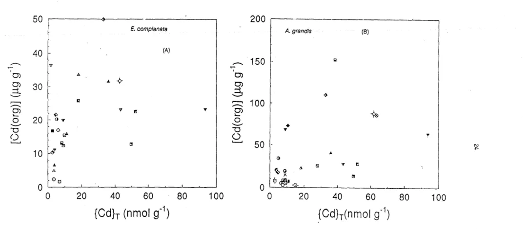
Cadmium concentrations in the tissues of the freshwater bivalves are much better related

to the parameters appearing in the right-hand side of Eqns (3) than to total sedimentary

cadmium, {Cd}T (compare Fig. 4 and 5). Indeed, when cadmium concentrations in the

bivalves are compared with {Cd}T' no significant relationships emerge (Fig. 5). The same

conclusion is reached when Cd concentrations in the bivalves are compared with cadmium

concentrations found in any sediment extract, whether or not the extractable Cd is

normalized with respect to sediment iron oxyhydroxide or organic carbon concentrations.

Such empirica1 normalizations have been advocated recently for the prediction of As, Cu,

Hg and Pb bioaccumulation in bivalves (Table 6: Langston 1980, 1982; Luoma and Bryan,

1978; Tessier

et al.,

1983; 1984), but they do not seem to be adequate for predicting Cd

accumulation

in

E.

complanata

and

A. grandis

for a large variety of lakes as here.

Prediction of [Cd(org)] with the sedimentary parameters appearing in Eqns. (3) is as

good as the prediction with the dissolved [Cd] and the inorganic ligand concentrations

(compare Figs. 3 and 4). However, use of sedimentary measurements offers considerable

advantages. The measurement of low dissolved Cd concentrations

in

freshwaters is difficult

and requires the use of trace metal-free techniques; possibilities of inadvertent

contamination are rampant. An additional problem is the temporal variation of dissolved Cd;

considerable effort would be needed to obtain representative mean values of total dissolved

Cd at each sampling site. By comparison, the measurement of {Cd}T' {Fe-ox}, rOM} and

lake pH is much simpler.

An

important point to note is that the geochemica1 constants x, y,

and

NOM· *KoM-Cd

determined in this study are specific to cadmium. These types of constants

should be metal-specific, and not organism-specific. Once they are determined accurately

for a given metal, they could

in

principle be used for predicting trace metals in any organism

that obtains its metal burden from the ambient water. For a specific organism, the only

requirement would then be to determine F and [M(org)]O (as in Eqn 5) from a proper

calibration. The geochemica1 constants are

in

fact used only to estimate

which is the

same for all the organisms at a given site.

40

---.

150 .

₃₀

::i.

::i.

₁₀₀

---.

"

20

-

_•

.,

()

0

,.

_{50 .}

10

"

°0

~~-0-!

0

0

0

20

40

60

80

100

0

20

40

60

80

100

{Cdh (nmol

g-1)

{Cdh(nmol

g-1)

Figure 5. Relationship between Cd concentrations in the tissues (whole organisms) of

E. complanata

(A) and

A. grandis

(B)

and total Cd concentrations in the sediments. Symbols represent various sampling sites.

N

.f'-lrganism

Metal

Prediction

Reference

'crobicularia

Pb

{Pb} extracted

{Pb}j{Fe} extracted

Luoma and Bryan, 1978

lana

with lN HCl

with lN HCl

(r=0.69)

(r=0.99)

crobicularia

Hg

{Hg}T

{Hg} extracted

{Hg} extracted with

Langston, 1982

lana

(r=0.72)

with lN HCl

_{HN03 jorganic content}

(r=-0.61)

(r=0.80)

crobicularia

As

{As} extracted

{As}j{Fe} extracted

Langston, 1980

lana

with

HCl

with lN HCl

(r=0.80)

(r=o. 96)

'acoma

Hg

{Hg} extracted with

Langston, 1982

1Zthica

_{HN0 3jorganic content}

lliptio

Cu

{Cu}T

{Cu} extracted

{Cu}j{Fe} extracted

Tessier

et al. , 1984

Jmplanata

(r=O.79)

_{with NH2OH.HCl}

_{with NH2OH.HCl}

(r=0.94)

(r=O.97)

'liptio

Pb

{Pb}T

{Pb} extracted

{Pb}j{Fe} extracted

Tessier

et al. , 1984

)mplanata

(r=O.77)

_{with NH2OH.HCl}

_{with NH2OH.HCl}

(r=0.87)

(r=0.96)

lOdonta

Cu

{Cu}j{Fe} extracted

Tessier

et al. , 1983

'andis

_{with NH2OH.HCl}

(r=0.92)

---,

N

In earlier studies, field measurements along trace metal gradients have shown that the

prediction of metal concentrations in estuarine and freshwater bivalves, [M(org)], was greatly

improved when the trace metal concentration extracted from the sediments was normalized

with respect to the iron oxide or organic matter content of the sediments (Table 5). Hence, the

ratios {Pb}/{Fe} and

{As}/{Fe},

all extracted with IN HCl, and the ratio {Hg extracted with

HN0

}/{OM}

were found to be the best predictors of lead, arsenic and mercury

concentrations respectively in the estuarine bivalve Scrobicularïa plana (Langston 1980, 1982;

Luoma and Bryan 1978). Similarly, the best predictors of Cu and Pb in the tissues of the

freshwater bivalves A. grandis and E. complanata were found to

he

the ratios {Cu}1 {Fe} and

{Pb}/{Fe} extracted with

a reducing reagent (Tessier

et

al. 1983, 1984). In other

words, according to these studies, trace metal concentrations in the organisms are best

expressed as:

[M(org)]

=

k ---

+

[M(org)]O

where k is a proportionality constant; {Sn} is the concentration of a sediment component n

(which can be Fe oxyhydroxides or organic matter); {Sn-Ml is the concentration of the trace

metal M associated with sediment component n; [M(org)]O is the intercept on the y-axis (which

is usually smaIl).

The present study offers a likely explanation for these findings. The studies of Langston

(1980, 1982) and Luoma and Bryan (1978) were performed in estuaries, where the pH is

relatively constant; the freshwater studies (Tessier

et

al. 1983, 1984) were carried out in three

lakes located

in

a restricted geographica1 area where the lake pH is relatively constant. In such

cases,

and

become approximate1y constant, and combination of either Eqn. (3a) or

(3b) with Eqn.! (5) 1eads to Eqn. (6). The success of sediment Fe or organic carbon as the

normalizing factor in these studies could be due to its dominance in the sorption of the

particular trace metal investigated. For example, the strong association of Pb (Lion

et

al.

Balistrieri and Murray 1982; Leckie

et

al. 1984) and of As (Aggett and Roberts 1986; Belzile and

Tessier 1990) with sedimentary iron oxyhydroxides is well documented; similarly, the affinity of

Hg for sediment organic matter (NRCC 1988) is well known.

From the preceding discussion, it follows that the observation of a strong relationship

between trace metallevels in a benthic species and sediment characteristics (e.g., extractable

metal concentration normalized with respect to the concentration of a sediment component like

Fe oxyhydroxides or organic matter) cannot be considered as evidence that the main route of

trace metal uptake is via ingestion of particulate material. Such relationships could also be

observed for organisms that obtain metal directly from the water, provided that i) the pH is

approximately constant over the study area; ii) the dissolved

in the water to which the

organisms are exposed is in sorptive equilibrium with the sediment component used for

normalization. A logical consequence is also that the ratios

{M}/{Fe}

or

{M}/{OM},

although

much better predictors than total sediment metal concentrations in sorne cases, are not

"universal" predictors in the sense that their application should be site-dependent (i.e.,

restricted to a narrow pH range).

5. CONCLUDING REMARKS AND RECOMMENDATIONS

We strongly believe that the development of deterministic models based on sound chemical

and biological principles constitutes the most promising approach to the prediction of trace

metal burdens

in

benthic organisms, and eventually

the prediction of metal effects on this

community. Provided such models explicitly incorporate the influence of major environ mental

variables on metal uptake, they should be of general applicability, i.e. they should be able to

predict the metal burden of benthos in lakes other than those used for their calibration. In

contrast, purely empirical models (black box models), based on statistical relationships only,

are useful means of reducing the experimental data but cannot be used to make predictions

beyond the original data set. The development of deterministic models has been hindered in

the past by our incomplete knowledge of the geochemical and biological processes that control

metal accumulation in aquatic organisms. There is no doubt that considerable effort should be

devoted to understanding these biogeochemical processes if we are to understand how

remedial actions will affect benthic organisms.

The present study represents an attempts to develop a deterministic model of general

applicability to predict bioaccumulation of trace metals in aquatic organisms. In the formulation

of the model, we use concepts derived from the free-ion model of metal-organism interactions,

the water or in 'the surficial oxic sediments. From a practica1 point of view, this approach has

yielded predictive equations for Cd accumulation in

A.

grandis

that require as input

geochemica1 variables readily measured in the bottom waters (PH) and in the sediments

({Cd}T' {Fe-ox} and {OM}). A most important point arising from the study is that relatively little

would be needed to establish predictive equations for metal burdens in benthic organisms once

the geochemica1 constants x, y,

and

are known accurately for the

metals of interest.

Severa! recommendations arise from our work:

1.

Determination of the geochemical constants.

The approach developed here for Cd could

also be extended to other trace metals. Since the geochemica1 constants x, y,

and

NOM· ·KOM-Cd

are involved in the prediction of cadmium accumulation by (and cadmium effects

on) various aquatic organisms, we think that appreciable effort should be devoted to their

accurate detennination; such an effort would yield a basis for good prediction of cadmium

availability to benthic organisms. For example, the following points are suggested:

- Time-averaged values (rather than single grab measurements; see Appendix) of dissolved

cadmium concentrations should be obtained at each site for the determination of the

geochemica1 constants.

- Possible means to improve the estimation of the free aquo ion concentration, [Cd2+], should

be investigated.

In

the present study, we have considered only dissolved inorganic ligands; the

role of dissolved organic matter in complexing Cd should be assessed and taken into account .

- Our knowledge of the precise sediment components responsible for the sorption of Cd should

be improved. Whicll, forms of organic matter are important for Cd sorption? In the present

study, we assumed'that it is total organic matter, since we use sedimentary organic carbon to

estimate {OM}. Which forms of iron oxyhydroxides are important for Cd sorption? The reagent

~OH·

HCL; 96°C) used in the present study to estimate {Fe-ox} extract the sum of

amorphous iron oxyhydroxides, ferrihydrite and lepidocrocite. More precise knowledge of the

forms of organic matter and iron oxyhydroxides responsible for the sorption, and the

constants. Are other sediment components (e.g. Mn oxyhydroxides) sometimes important for

Cd sorption? In the present study, we assumed that only organic matter and Fe oxyhydroxides

were important for sorbing Cd.

- The number of sites where Teflon sheets are used to collect diagenetic iron oxyhydroxides

(and associated Cd) should be increased; these experimental data are needed to calculate the

geochemical constants x and Npe ' ·Kpe-Cd' and hence indirectly to calculate y and NOM' ·KaM-Cd

(see Appendix for the details of the calculation). In the present study, only a limited number of

sites (8) were investigated with the Teflon collection technique.

2. Reimement of the geochemical model. Note that the considerations raised for Cd could

also be extended to other trace metals. The prediction of [Cd(org)] from sedimentary

measurements depends on how accurately the geochemical model can relate [Cd

in the

ambient water to sedimentary parameters. The geochemical model used here is still relatively

crude, and further work to refine it can be suggested.

- Our understanding of the nature of the sorption processes could be improved. Is it adsorption,

surface precipitation, co-precipitation? In the present study, we assumed that [Cd

is related

to sediment components by overall surface complexation reactions (see Eqn 2 in the Appendix)

suggested for adsorption of trace metals on hydrous metal oxides (Benjamin and Leckie, 1981).

Identification of the precise processes might lead to better expressions relating [Cd

to

sedimentary components.

- Effort should be devoted to identify the solid phases responsible for binding [Cd]. Once they

are known, better geochemical models could

he

developed to relate [Cd2+] to sediment

components. For example, aIl the experimental data on the adsorption of Cd on a given iron

oxyhydroxide can be described with a set of intrinsic acidity constants, intrinsic adsorption

constants for Cd on this solid, density of sites and specifie surface area of this solid, and a

description of the pOtential-surface charge relationship (Dzombak and Morel, 1990). Laboratory

experiments with pure solid phases have shown that values of these parameters vary from one

Fe oxyhydroxide to the other.

If

the exact forms of Fe oxyhydroxides present in natural

sediments were known, we could use these laboratory-derived parameters in a refined

geochemical mode!. Since this information is not yet available, we adopted in the present study

a semi-empirical approach where an overall reaction (see Eqn 2 in the Appendix) is used to

3. Biomonitors. Aquatic organisms have been proposed as "biomonitors" for trace metal

pollution. Our results raise several points and recommendations for further work.

- Freshwater bivalves have been proposed for biomonitoring purposes (Forester, 1980).

According to our results,

A. grandis,

and probably

E. complanata,

do not react rapidly to

changes in ambient Cd, Cu and Pb concentrations. For example,

A. grandis

specimens

transferred to a polluted lake had not attained, after three years, the metal burdens of

indigenous specimens in the polluted lake. Thus, freshwater bivalves will probably be useful for

monitoring long-term trends in metal pollution. The suitability of smaller organisms (e.g. in sect

larvae) should be investigated for monitoring trace metal variations in the environ ment on a

short-term basis.

- Use of organisms for biomonitoring trace metals requires that the relationships between metal

concentrations in the organisms (or in a specific tissue) and their external environ ment: i) be

well known; ii) apply to sites other than those used for calibration; iii) apply to environ mental

conditions other than those used for the calibration.

In

our opinion, this generality can be

obtained only if the relationships between tissue metal concentration and predictive

environ mental variables are derived from sound biological and chemical princip les. This critical

point has been overlooked in the past and should be addressed explicitly.

- Figure 3 shows that prediction of Cd concentration in the tissues of

A. grandis

from

sedimentary variables is acceptable for a large number of aquatic environments (over a

geographical aJrea of about 350 000 km

in this case); this is an example of a predictive

relationship based on biological and chemical processes. Admittedly, the relationships between

[Cd(org)] and the sedimentary parameters could be improved by a better determination of the

geochemical constants and a refmement of the geochemical model, as discussed above.

Similar approaches to the one developed for the study of Cd in

A. grandis

could be adopted for

the study of other trace metals in other aquatic organisms.

ACKNOWLEDGEMENTS.

Financial SUpport from the Ontario Ministry of the Environment is acknowledged. We thank S.

Hinch, B. Lazerte and G. Mackie for providing helpful information with regard to the selection of

study lakes.

REFERENCES.

Aggett, J. and L. S. Roberts (1986). Insight into the mechanism of accumulation of arsenate and

phosphate in hydrolake sediments by measuring the rate of dissolution with

ethylenediaminetetraacetic aeid (EDTA). Environ. Sei. Technol. 20: 183-186.

Balistrieri,

L.

S. and J. W. Murray (1982). The adsorption of Cu, Pb, Zn and Cd on goethite from

major ion seawater. Geochim. Cosmochim. Acta 46: 1253-1265.

Belzile, N. and A. Tessier (1990). Interactions between arsenic and iron oxyhydroxides in

lacustrine sediments. Geochim. Cosmochim. Acta 54: 103-109.

Belzile, N., R.R. De Vitre and A. Tessier (1989).

In situ

collection of diagenetic iron and

manganese oxyhydroxides from natural sediments. Nature

376-377.

Benjamin, M.M. and J.O. Leckie (1981). Multiple-site adsorption of Cd, Cu, Zn, and Pb on

amorphous iron oxyhydroxide. J. Colloid Interface Sei. 79:209-221.

Campbell, J. and R. D. Evans (1991) Cadmium concentrations

in

the freshwater mussel

(Elliptio

complanata)

and their relationship to water chemistry. Arch. Environ. Contam. Toxicol. 20:

125-131.

Carignan, R. (1984). Interstitial water sampling by dialysis: Methodological notes. Limnol.

Oceanogr.29:667-670.

Carignan, R., F. Rapin and A. Tessier (1985). Sediment porewater sampling for metal analysis:

a comparison of techniques. Geochim. Cosmochim. Acta 49:2493-2497.

DiToro, D. M., J. D. Mahony, P. R. Kirchgraber, A. L. O'Byme,

L.

R. Pasquale and D. C. Piccirilli

(1986). Effects of nonreversibility, partic1e concentration, and ionic strength on heavy metal

sorption. Environ. Sei. Technol. 20: 55-61.

Dzombak, D.A. and F.M.M. Morel (1990). Surface complexation modeling. Hydrous ferric oxide.

Wiley.