Fault and natural fracture control on upward fluid migration: insights from a shale gas
1
play in the St. Lawrence Platform, Canada
2
Ladevèze, P. 1,a,b, Rivard, C. b, Lavoie, D.b, Séjourné, S.c, Lefebvre, R.a, Bordeleau G.b 3
4 a
INRS, Centre Eau Terre Environnement, 490 rue de la Couronne, Quebec City, QC G1K 9A9, 5
Canada 6
b
Geological Survey of Canada – Quebec, 490 rue de la Couronne, Quebec City, QC G1K 9A9, 7
Canada 8
c
Enki GéoSolutions, Montréal, Canada 9
1
Corresponding author: [email protected] 10
Abstract
11
Environmental concerns have been raised with respect to shale gas exploration and production, 12
especially in eastern Canada and northeastern United States. One of the major public concerns 13
has been the contamination of fresh water resources. This paper focuses on the investigation of 14
possible fluid upward migration through structural features in the intermediate zone (IZ), located 15
between a deep shale gas reservoir and shallow aquifers. The approach provides insights into how 16
such an investigation can be done when few data are available at depth. The study area is located 17
in the shale dominated succession of the St. Lawrence Platform (eastern Canada), where the Uti-18
ca Shale was explored for natural gas between 2006 and 2010. Detailed analyses were carried out 19
on both shallow and deep geophysical log datasets providing the structural attributes and prelimi-20
nary estimates of the hydraulic properties of faults and fractures. Results show that the active 21
groundwater flow zone is located within the upper 60 m of bedrock, where fractures are well in-22
terconnected. Fractures from one set were found to be frequently open in the IZ and reservoir, 23
providing a poorly connected network. The fault zones are here described as combined conduit-24
barrier systems with sealed cores and some open fractures in the damage zones. Although no di-25
rect hydraulic data were available at depth, the possibility that the fracture network or fault zones 26
act as large-scale flow pathways seems very unlikely. A conceptual model of the fluid flow pat-27
terns summarizing the current understanding of the system hydrodynamics is also presented. 28
255 words 29
Keywords: natural fractures; faults; upward fluid migration; shale gas; St. Lawrence Platform
30 31
1 Introduction
32
Shale gas development in North America has raised strong local environmental concerns, largely 33
in relation to potential contamination of fresh water resources during hydraulic fracturation oper-34
ations (BAPE 2014; CCA 2014; EPA 2016). One of these concerns is associated with potential 35
upward fluid migration from deep geological reservoirs to shallow aquifers through preferential 36
pathways such as natural fractures and faults (Lefebvre 2016). Fluids of concerns include hydrau-37
lic fracturing fluids, gases (mostly methane) and formation brines (Birdsell et al. 2015). Although 38
the presence of natural preferential pathways that could affect fresh water quality is of particular 39
anxiety to the population, it is now recognized among the experts that the well casing integrity is 40
the major concern with respect to potential upward fluid migration (Dusseault and Jackson 2014; 41
Lefebvre 2016). Nonetheless, the need for a better description and representation of the potential 42
preferential flow pathways in hydrogeological models to assess the risk of upward fluid migra-43
tion has been stressed by many researchers (Gassiat et al. 2013; Kissinger et al. 2013; Birdsell et 44
al. 2015; Reagan et al. 2015; Grasby et al. 2016). So far, most authors have used mean values to 45
obtain representations of different hydrogeological systems for their simulations. While these 46
provide interesting insights into mechanisms and conditions that could lead to aquifer contamina-47
tion, there is a critical need for field-based research studies in developing a methodology aimed at 48
identifying natural preferential migration pathways using multiple data sets (Jackson et al. 2013). 49
In particular, very little work has focused on the characterization of fracture networks in the in-50
termediate zone (IZ), which is located between shallow aquifers (usually in the upper 200 m) 51
used for water supply and deep hydrocarbon reservoirs (usually deeper than 1000 m). However, 52
this geological interval controls the shallow aquifer vulnerability to activities carried out at depth. 53
In the St. Lawrence Platform (Quebec, Canada), shale gas exploration targeting the Utica Shale 54
was conducted between 2006 and 2010 until a de facto moratorium on hydraulic fracturing came 55
into force, in response to strong environmental concerns (BAPE 2014). In this context, the objec-56
tive of this study was to identify the potential for fluid upward migration through natural frac-57
tures and faults in the Saint-Édouard area, 65 km south-west of Quebec City (Fig. 1), a region 58
where a promising shale gas well had been drilled. 59
Multisource data including shallow and deep log datasets, core data and seismic data were exam-60
ined to assess the geometry and potential hydraulic properties of the structural features that affect 61
the sedimentary succession, including the IZ. A special focus was placed on the presence and 62
properties of open fractures and permeable faults. Because hydraulic data are currently not avail-63
able in the study area for depths below surficial aquifers, as is the case in most shale gas plays, 64
this paper discusses how existing common field datasets can help to understand the hydraulic 65
behavior of the fractures and faults that cut through a sedimentary succession. A precise quantita-66
tive assessment of the hydraulic properties of these structural discontinuities is beyond the scope 67
of the paper. Our approach rather provides semi-quantitative insights into the possibility of up-68
ward migration through fractures and faults, based on available field observations and knowledge 69
acquired from the geological context. 70
2 The St. Lawrence Platform and St-Édouard study area
71
2.1 Regional geological setting
72
The St. Lawrence sedimentary Platform is divided into two tectonostratigraphic domains (St-73
Julien and Hubert 1975): the autochthonous and the parautochthonous domains (Fig. 1). In this 74
paper, the term St. Lawrence Platform (SLP) refers to the area roughly located between Montreal 75
and Quebec City (Province of Quebec, Canada). 76
In the autochthonous domain, Cambrian-Lower Ordovician clastic and carbonate units of the 77
Potsdam and Beekmantown groups unconformably overly the Grenvillian crystalline rocks 78
(Lavoie et al. 2012). During the Middle to Late Ordovician, these units were overlain by the car-79
bonate units of the Chazy, Black River and Trenton groups and by the calcareous shale of the 80
Utica Shale (Lavoie 2008). The uppermost preserved units of the SLP consist of the Upper Ordo-81
vician turbidite deposits of the Lorraine Group and the molasse units of the Queenston Group. 82
The Sainte-Rosalie, Lorraine and Queenston groups were slightly deformed in the regional-scale 83
Chambly-Fortierville syncline. A normal fault system also intersects the units throughout the au-84
tochthonous domain (Rivière Jacques-Cartier fault) (Fig. 1). 85
The parautochthonous domain corresponds to rocks that were displaced in a southeast-dipping 86
system of thrust faults that display imbricated thrust fan geometries (St-Julien et al. 1983; 87
Séjourné et al. 2003; Castonguay et al. 2006). The parautochthonous units were also deformed by 88
some northeast-striking folds. The Aston fault and the Logan’s Line regional thrust-faults delimit 89
the parautochthonous domain to the NE and SW, respectively (St-Julien and Hubert 1975; 90
Globensky 1987). The Logan’s Line represents the structural limit between the SLP (or parau-91
tochthonous domain) and the Appalachians (or the allochthonous domain) where rocks were dis-92
placed northwestwardly along the Appalachian’s thrust planes (Tremblay and Pinet 2016). In the 93
Saint-Édouard area, recent seismic reinterpretation of vintage industry data (Konstantinovskaya 94
et al. 2009; Lavoie et al. 2016) showed that the parautochthonous domain forms a triangular zone 95
delimited by a NW-dipping backthrust to the northwest and by a SE-dipping thrust fault to the 96
southeast (Logan’s Line) (Fig. 1). 97
The Utica Shale is considered an excellent conventional hydrocarbon source rock and an uncon-98
ventional gas reservoir (Lavoie et al. 2008; Lavoie et al. 2014). It is mostly overlain by the fine-99
grained units of the Lorraine Group and it is laterally equivalent to the Lotbinière Formation in 100
the northern part of the autochthonous domain, while it is structurally overlain by the Les Fonds 101
Formation in the parautochthonous domain (Fig. 1). The Lotbinière and Les Fonds formations 102
(Fig. 2) display a dominant lithofacies similar to, and are also time-correlative with, the Utica 103
Shale (Lavoie et al. 2016). However, Lorraine Group units are made of gray to dark-grey shales 104
with metre- to centimetre-thick siltstone interbeds (Clark and Globensky 1973; Globensky 1987). 105
Shales from the Lorraine Group are more clayey than those of the Utica Shale (Lavoie et al. 106
2008). The siltstone interbeds are mostly concentrated in the upper part of the Nicolet Formation 107
(Lorraine Group) (Clark 1964; Clark and Globensky 1973; Séjourné et al. 2013). The maximum 108
thickness of these siltstone-rich successions is unknown. Field observations showed that the silt-109
stone-rich zones are locally concentrated in recurring multiple intervals that display thicknesses 110
of up to 15-20 m in the upper part of the formation (Fig. 2). The siltstone proportion decreases 111
with depth, from up to 80% of siltstones in the upper part of the unit, to 30-40% in the middle 112
part, to almost no siltstone interbeds at the base of that formation (Séjourné et al. 2013). Given 113
the limited outcrop availability and the lack of clear marker beds, the lateral extension of these 114
interbeds in the shale-dominated succession is largely unknown. 115
The stratigraphic (sensu stricto) intermediate zone is provided by the fine-grained clastics of the 116
Lorraine Group and also by the Utica Shale time- and facies correlative Lotbinière and Les Fonds 117
formations to the north and south, respectively. 118
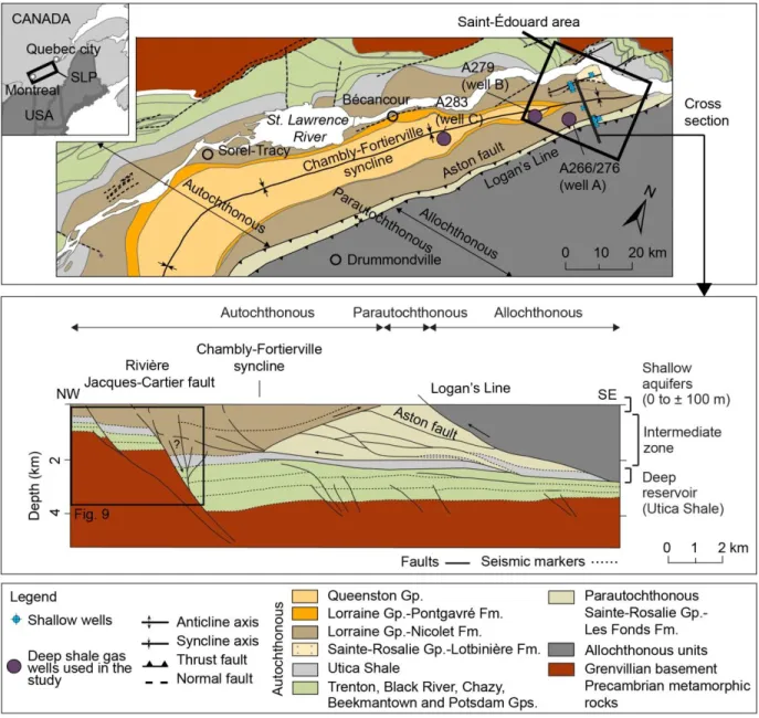
Fig. 1 Location of the study area and its geological context (geological maps adapted from Clark
and Globensky (1973); Globensky (1987); Slivitzky and St-Julien (1987); Thériault and Beauséjour (2012); Konstantinovskaya et al. (2014a). Gp.: Group; Fm.: Formation; SLP: St. Lawrence Platform. The structural cross-section is from Lavoie et al. (2016) that is based on vintage industry data.
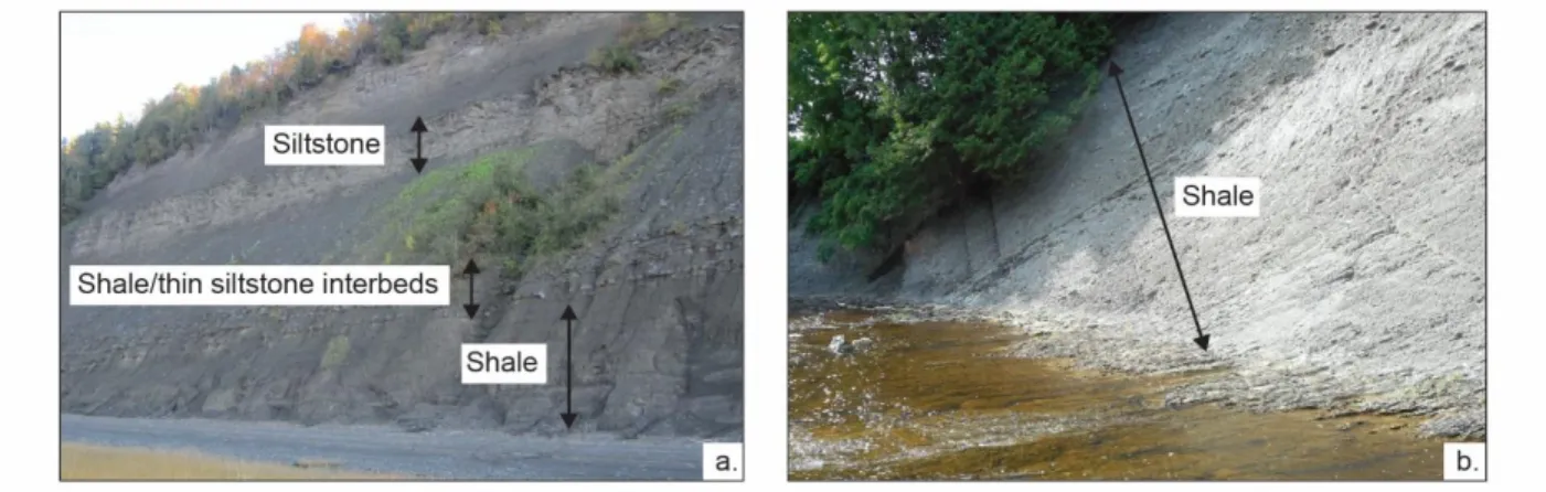
Fig. 2 Examples of outcropping IZ units of the Saint-Édouard area: a. Lorraine Group (Nicolet
Formation): grey-black shales with thick siltstone interbeds and b. Les Fonds Formation: black shales.
2.2 Conceptual models of the natural fracture network
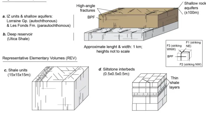
121
Conceptual models of the fracture network that affects the geological units of the Saint-Édouard 122
area were proposed in Ladevèze et al. (2018) (Fig. 3). These models are based on observations 123
made in 15 outcrops of various orientations, as well as in 11 shallow observation wells and 3 124
deep shale gas wells. Three sets of high-angle fractures were identified: F1, F2 and F3, their 125
numbering is based on their relative timing (F1 is the oldest). Bedding parallel fractures were also 126
observed in the shallow interval. The F1 and F2 fractures strike respectively NE and NW, are 127
perpendicular to each other and orthogonally crosscut the bedding planes. They can be found 128
everywhere throughout the shallow and deep intervals. The third fracture set (F3) strikes WNW 129
and is sub-vertical (dip>80°), irrespective of the bedding plane attitudes. F3 fractures are more 130
sparsely distributed and were mostly observed in the Utica Shale. Higher fracture densities were 131
found in the deep reservoir compared to the lower portion of the IZ where some log data are 132
available from shale gas wells (Fig. 3a and b). Based on the similarities of the fracture sets and 133
knowledge of the geologic history of the region, it was concluded that shallow and deep fracture 134
datasets could be used as analogs for the intermediate zone for which very little data are availa-135
ble. 136
In siltstone units, fractures are stratabound, contrary to those in shale units. Fracture densities are 137
also higher in siltstone units (compared to shale units) and in the calcareous Utica Shale (com-138
pared to the more clayey Lorraine Group units). This can be related to their relative difference in 139
brittleness (Séjourné 2017; Ladevèze et al. 2018). 140
To summarize and integrate all the information and knowledge acquired on the fracture network, 141
representative elementary volumes (REV) were proposed for the different geological intervals 142
(Fig. 3a and b) and for the shale and siltstone units (Fig. 3c and d). The sizes of the REVs were 143
defined based on fracture length and spacing in the shale and siltstone units (Lorraine Group) of 144
the area as originally proposed in Oda (1985, 1988) and Odling et al. (1999). It must be kept in 145
mind that these REVs are theoretical volumes that are considered representative of a given unit 146
based on available fracture data. 147
There is a lack of field evidence for the vertical extent of structural discontinuities due to the lim-148
ited size of the outcrops and to the fact that borehole data do not provide any direct observation 149
of fracture lengths (Ladevèze et al. 2018). Due to these limitations, and the near absence of data 150
for the intermediate zone, the vertical extension of natural fractures, which represents a critical 151
parameter to assess aquifer vulnerability, still remains elusive (Ladevèze et al. 2018). 152
153
2.3 Key elements for the hydrogeological context
154
In the Saint-Édouard area, bedrock hydraulic conductivities (K) vary between 10-5 and 10-9 m/s 155
according to pneumatic slug tests carried out on 11 shallow wells (open to bedrock) (Ladevèze et 156
al. 2016). Higher K values were obtained in wells located in the autochthonous domain, with a 157
marked correlation associated with the presence of siltstone interbeds. Wells in the parautochtho-158
Fig. 3 Conceptual models of the fracture network in the Saint-Édouard area. The regional
frac-ture pattern is represented in a. for the shallow aquifers and intermediate zone (IZ) units; in b. for the deep reservoir. The fracture pattern is also represented using REVs at a much more local scale for: c. shale units and d. siltstone interbeds. BPF: Bedding-parallel fractures; F1, F2 and F3: high-angle fracture sets; the numeration is based on the relative timing of the fracture sets formation. Figure modified from Ladevèze et al. (2018).
nous domain displayed lower K values, as they only intersected shale units that are highly folded 159
and faulted. 160
The occurrence of brines migrating into the shallow aquifer was documented in the vicinity of the 161
Rivière Jacques-Cartier normal fault (Fig. 1) (Bordeleau et al. 2018a; Bordeleau et al. 2018b). 162
The authors indicated that the presence of this brine in a few shallow (50 m) wells does not nec-163
essarily point to the existence of a large-scale upward migration pathway from the gas reservoir. 164
This brine contribution would rather result from regional groundwater flow originating in the 165
Appalachian uplands and circulating at a maximum depth of a few hundred meters. Hence, 166
groundwater would flow, at least to some extent, into formations containing old saline water, 167
then discharge in the vicinity of the Rivière Jacques-Cartier fault system (Bordeleau et al. 168
2018b). The concentrations of thermogenic methane measured in wells close to this normal fault 169
were not higher than those in wells located elsewhere in the region and its isotopic composition 170
was different than that of the Utica Shale (Bordeleau et al. 2018b). The thermogenic gas occur-171
rences in the shallow aquifer of the Saint-Édouard area are interpreted to be sourced from the 172
shallow shale units themselves (thermogenic gas being trapped in pores) (Lavoie et al. 2016; 173
Bordeleau et al. 2018b). 174
3 Methodology
175
A three-step methodology was employed in this study. First, the presence and potential properties 176
of open natural fractures within the intermediate zone was assessed to the best of our knowledge 177
given the available data, to evaluate their impact on groundwater flow dynamics. Second, the 178
architecture and properties of the regional fault zones were examined to infer their hydraulic 179
properties, in order to assess their hydraulic behavior (for instance, whether they are permeable or 180
for upward fluid migration from the shale gas reservoir to the shallow aquifer based on available 182
field data. 183
The general term “fracture” encompasses a large number of structures (Peacock et al. 2016). 184
Here, the term “fractures” refers to meter scale planar discontinuities within the rock mass with-185
out visible displacement. To the contrary, the term “faults” here refers to discontinuities that 186
show a displacement. In the SLP, faults were defined both at a local (meter) and a regional (kilo-187
meter) scale. 188
3.1 Data collection
189
In this study, the focus was placed on structural features that could act as preferential upward 190
fluid flow pathways. In this perspective, fracture and fault physical properties (aperture, cementa-191
tion), cross-cutting relationships and extent/distribution were carefully examined using all availa-192
ble data. For the Saint-Édouard area, the datasets comprised data from field observations and 193
measurements, core samples, digital logs (shallow and deep wells) and seismic profiles. 194
A total of 15 shallow (from 15 to 145 m within the shallow fractured rock aquifer) observation 195
wells were drilled into the Lorraine and Sainte-Rosalie groups (Ladevèze et al. 2016), of which 196
11 were logged using acoustic and optical televiewer tools (Crow and Ladevèze 2015). Core 197
samples were also collected in seven of these boreholes. To complete the dataset at greater depth 198
in the sedimentary succession, Formation Micro Imager (FMI) logs acquired in three deep shale 199
gas wells: well A (A266/A276 - Leclercville n°1), B (A279 - Fortierville n°1) and C (A283 - Ste-200
Gertrude n°1) (see Fig. 1 for their location). The FMI logs were recorded in both the vertical and 201
horizontal portions of the three studied shale gas wells. The logged intervals (true vertical depth) 202
range from 1470 to 2010 m for well A, 560 to 2430 m for well B and 590 to 2010 m for well C. 203
These intervals include the Utica Shale and variable portions of the overlying Lorraine Group. In 204
the horizontal portion of these wells (“horizontal legs”), the logged intervals span across 1000, 205
970 and 920 m in the Utica Shale, respectively. These horizontal portions, also in true vertical 206
depths, were drilled approximatively between 1900-1950, 2150-2250 and 1800-1850 m below 207
the ground surface for wells A, B and C respectively. These FMI logs were provided by industry. 208
3.2 Characterization of open fractures
209
3.2.1 General approach
210
The Lorraine Group and the Utica Shale have low matrix porosity (geometric mean total porosity 211
~2.9%; BAPE 2010; Nowamooz et al. 2013; Séjourné et al. 2013; Séjourné 2015) and permeabil-212
ity (geometric mean permeability: 10-20 m2, i.e., 10-5 mD or milliDarcy; BAPE 2010 and Séjourné 213
et al. 2013). As the matrix of these shales is very tight (Haeri-Ardakani et al. 2015; Lavoie et al. 214
2016; Chen et al. 2017), it appears that significant fluid flow circulation could only occur through 215
open fractures. The presence of open fractures in the rock mass was thus investigated using the 216
conceptual models of the fracture network developed in Ladevèze et al. (2018) (Fig. 3) with the 217
aim of identifying potential flow pathways. 218
The main characteristics of the natural fractures within the study area that could impact fluid mi-219
gration are summarized in Table 1. These characteristics should be taken into consideration in 220
assessment studies investigating potential upward migration. 221
Table 1 Summary of natural fracture network characteristics in the intermediate zone (IZ) that
222
may either enhance or limit upward fluid migration 223
Natural fracture characteristics that were examined
Enhance fluid migration
Limit fluid migration
tures in multiple sets limited interconnection
Open fractures attributes
Fracture sets versus con-temporary in situ SHmax
(maximum horizontal stress) orientations
Fracture planes are parallel to SHmax
Fracture planes are orthog-onal to SHmax
Distribution of open fractures in the
sedimen-tary succession
High density of open fractures
Sparsely distributed open fractures
Fracture aperture in the deep intervals (reservoir
and IZ)
Large apertures Small apertures
Open fractures and hy-draulic properties of the rock mass Fracture porosity in a context of low matrix
porosity rock
High fracture porosity Low fracture porosity
Fracture permeability (k) High fracture k Low fracture k
224
3.2.2 Open fracture attributes
225
Open fractures were identified in shallow observation wells and in both vertical and horizontal 226
sections of the deep shale gas wells. Fracture observations are, however, affected by an important 227
sampling bias related to their orientation versus that of the borehole (sub-vertical fractures are 228
under-sampled by vertical wells). Another important bias is that fracture aperture may be en-229
hanced and closed natural fracture planes artificially opened during drilling operations (due to the 230
rotation of the drill bit, to the injection of pressurized drilling fluid into the open borehole, or to 231
the pressure exerted by the regional stresses). Therefore, when interpreting statistics on the pres-232
ence of open fractures in a fracture dataset, only general trends were considered. 233
Measurements of fracture apertures were seldom possible in shale outcrops due to surficial and 234
shallow subsurface processes such as frost weathering and fracture filling with surficial materials, 235
but it was quite often possible in well logs. In shallow wells, fracture aperture is directly measur-236
able on acoustic televiewer (ATV) images (with a precision of around 1 mm), as open fractures 237
generally display low amplitudes and high travel times (Davatzes and Hickman 2010). As 238
closed/cemented fractures rarely produce geometric irregularities on the borehole wall, optical 239
logs were also used to facilitate their identification in shallow wells. In deep shale gas wells, the 240
aperture can only be observed indirectly using FMI data through resistivity contrasts. Since open 241
fractures are filled with conductive fluids (brines or drilling mud), they display more conductive 242
signatures than quartz- or calcite-cemented (healed) fractures. Resistive healed fractures also dis-243
play a “halo effect” caused by the resistivity contrast between the filling and the host rock, which 244
helps their identification (Thompson 2009). 245
Fracture apertures, estimated from shallow (ATV) and deep (FMI) well logs, are here called “ap-246
parent apertures” due to the sparsely distributed measurements that were available and because of 247
the limitations of the methods (listed in Appendix 1). When comparing shallow ATV and deep 248
FMI datasets, apparent apertures are markedly higher in the shallow aquifer (at least more than 249
three orders of magnitude higher than in the deep shale gas wells). However, the magnitude of 250
this difference must be interpreted with caution as the results were derived from two different 251
estimation methods that both have important limitations (also listed in Appendix 1). In FMI logs, 252
fracture apertures are approximately one order of magnitude higher in the lower portion of the IZ 253
than in the deep reservoir. Fracture aperture estimates from FMI logs were available for both F1 254
and F3 fractures and there was no significant difference in aperture values when comparing these 255
two fracture sets. 256
Finally, open and closed fracture densities were calculated along the wells using a counting win-257
dow. The fracture densities were then normalized by the window length, so as to be expressed as 258
a number of fractures per distance unit (one meter). More details on this approach are provided in 259
Ladevèze et al. (2018). 260
3.2.3 Fracture porosity and permeability
261
Hydraulic properties related to open fractures (fracture porosity and permeability) within the IZ 262
are critical when investigating potential upward fluid migration. However, a quantitative estima-263
tion of the hydraulic properties of the fractures is beyond the scope of this paper. The aim of this 264
section is to assess semi-quantitatively the contribution of fractures to groundwater flow through-265
out the sedimentary succession, combining the conceptual model of the fracture pattern with 266
available data inferred from well logs. Hydraulic property values were estimated using the exist-267
ing datasets from the shallow aquifer (0-60 m within bedrock), the lower portion of the IZ (verti-268
cal well between 550 and 2000 m) and the reservoir (horizontal well). 269
The siltstone interbeds are mostly concentrated in the upper part of the Lorraine Group (see sec-270
tion 2.1) and because the focus of this study is on upward migration from the deep reservoir, the 271
hydraulic properties of the siltstone units are not discussed here. Hydraulic properties for the IZ 272
were thus estimated according to the REV of the shale units (Fig. 3c). To obtain representative 273
values for hydraulic properties, the proportion of open fractures in each set and the median values 274
of fracture spacing provided in Ladevèze et al. (2018) were used. Median values were preferred 275
over their mean as the fracture spacing distributions exhibit a few extreme values. In addition, as 276
no precise estimates of the fracture length are available (see section 2.2), the assumption was 277
made that fractures crosscut the REV throughout its length (15 m). As a consequence, results 278
obtained with this approach could be considered as an upper bound for realistic hydraulic proper-279
ty estimates.While the same fracture network (F1, F2 F3 and bedding plane fracture sets) was 280
assumed to be present throughout the sedimentary succession, its geometric properties, found 281
using mainly datasets from the shallow and deep intervals, can also be considered valid for the 282
intermediate zone (Ladevèze et al. 2018). However, when considering hydraulic properties, two 283
additional parameters must be taken into account: the variations in proportion of open fractures 284
and the variations in fracture apertures. Three assumptions are proposed here to assess the hy-285
draulic properties of the IZ based on the shallow and deep datasets. First, F1 fractures are consid-286
ered as the dominant fracture set in the IZ (based on results of the well log analysis showing that 287
open fractures in the deep interval belong mainly to this set). Second, the proportion of open F1 288
fractures observed in the reservoir is considered as an upper limit for the proportion of open F1 289
fractures in the lower portion of the IZ. These two assumptions are reasonable given that 1) the 290
permeability anisotropy is stress dependent (Barton et al. 1995; Ferrill et al. 1999), 2) according 291
to the in situ stress conditions in the SLP (Konstantinovskaya et al. 2012) (present-day maximum 292
horizontal stress -SHmax- is oriented NE-SW), fractures that are aligned with the SHmax are more
293
likely to be open (here, the NE striking F1 fractures, which is consistent with field observations 294
in the reservoir when neglecting the small proportions of open F2 and F3 fractures) and 3) an 295
increase in the magnitude of SHmax with depth is likely to open a higher proportion of fractures
296
that are parallel with this stress orientation (here, the proportion of open F1 fractures is likely to 297
increase with depth in the IZ and reservoir). Finally, the third assumption is that apertures esti-298
mated in the shallow aquifer can be used as proxies to estimate an upper bound for hydraulic 299
properties of the upper portion of the IZ. In fact, the fracture apertures in the upper part of the IZ 300
should be smaller than those from the shallow aquifers because processes such as uplift, decom-301
paction and erosion may likely enhance the aperture of F1 fractures in the shallow interval. The 302
degree of overestimation is, however, unknown. 303
The fracture porosity of the shale units within the Saint-Édouard area were estimated in shallow 304
aquifers and at depth using Eqn (1): 305 1 N i i i n b L
(1) 306 with i i L n s (2) 307In Eqn (1), θ is the fracture porosity; i the fracture set (F1, F2, F3 or BPF); ni the number of open
308
fractures from set i; bi is the aperture of the fractures from set i. and L is the length of the REV
309
(15 m). In Eqn (2), si is the median spacing for fractures from set i.
310
Since very few F3 fracture spacing measurements were available from outcrops, data from the 311
horizontal section of deep wells were used for the median spacing of F3 (as proposed in 312
Ladevèze et al. (2018)). This value represents again an upper bound as these structures are likely 313
to be more sparsely distributed in the IZ and shallow aquifer than in the reservoir. For the porosi-314
ty estimates in the shallow aquifers, fractures from sets F1, F2 and F3 were considered open; in 315
the IZ and in the reservoir, only F1 fractures were considered open. 316
Direct estimates of the hydraulic conductivity (K) were obtained in 14 shallow bedrock wells of 317
the Saint-Édouard area using slug tests (Ladevèze et al. 2016). No direct measurement of K be-318
low 150 m from the surface was available in the study area. Drill-stem tests could not be per-319
formed in wells A, B and C due to the low permeability of the rock. Thus, the relationship be-320
tween fracture aperture and K of the cubic law was used (Snow 1968). This model considers lam-321
inar flow between two parallel plates. The cubic law is either used to estimate K of a fracture us-322
ing its aperture or to obtain its aperture (“hydraulic aperture”) using a known K value (generally 323
field-based). This relationship can also be extended to estimate the hydraulic conductivity of a 324
fracture system by considering regular sets of parallel fractures (Bear 1993). This concept is con-325
sistent with the fracture network presented in Figure 3 (Fig. 3c) when only considering open F1 326
fractures. The relationship takes the form of Eqn (3). The use of permeability (k) was preferred 327
over hydraulic conductivity (K) at depth because the presence of a multiphase fluid flow system 328
(with oil/gas and brines) makes the use of K less relevant. The parameter k is only a function of 329
the medium (contrary to K that is a specific application of k to fresh water), which is thus more 330
appropriate in this case. The k values were calculated using Eqn (4). 331 2 12 b g K
(3) 332 and k K g (4) 333In Eqn (3), b is the aperture (in meters), θ is the fracture porosity (see Eqn 1), ρ is the fluid densi-334
ty in kg/m3, µ is the dynamic viscosity in Pa.s and g is the gravitational acceleration (9.81 m/s2). 335
For comparison with available literature values on deep formations, K values available for the 336
shallow interval were converted into permeability (k) using Eqn (3) and the thermo-physical 337
properties of water. These properties were estimated using water temperatures at depth according 338
to the mean geothermal gradient proposed in Bédard et al. (2014) for the SLP (23.0°C/km). 339
3.3 Characterization of fault zones
340
3.3.1 General approach
341
A fault zone is generally made up of a fault core surrounded by a damage zone, each of these 342
structures being either a barrier to, or a conduit for, fluid flow (Caine et al. 1996; Bense and 343
Person 2006; Bense et al. 2013). Fault zones affecting siliciclastic rocks thus generally display 344
permeability anisotropy (Odling et al. 2004). Based on available field datasets, the potential con-345
tribution to fluid flow circulation of the core and damage zones was examined in this study. It 346
must be emphasized that here only the natural conditions are studied based on existing and avail-347
able data. However, fault behaviour can be modified depending on present-day stress change and 348
pore-pressure increase related to fluid injection operations during hydraulic fracturing. If pore 349
pressure increases, effective stresses decrease and the fault zone, which could have been sealed 350
before these operations, can become critically stressed and reactivated (e.g, induced seismicity), 351
thereby potentially facilitating fluid migration along this fault. The topic of fault behavior in a 352
context of fluid injection operations is not addressed here. 353
Since no deep hydraulic tests were performed in the study area, the scope of this section is thus to 354
provide insights into how the available data (borehole data, seismic data, and core analysis data 355
such as the clay content) can help understand the fault zone behavior and whether the fault zones 356
could facilitate upward fluid circulation through the sedimentary succession. 357
To analyse the control exerted by fault zones on groundwater flow dynamics, an integrated inter-358
pretation based on the existing datasets and previous studies of faults in the SLP was done. First, 359
it must be noted that if a fault zone were to correspond to a flow pathway, its architecture would 360
affect the fluid travel time. Therefore, architecture of the fault zones were analysed using the 361
available structural cross-section in the study area (Lavoie et al. 2016). For this work, we follow 362
the generally accepted hypothesis that fault planes that are aligned with the maximum horizontal 363
stress (SHmax) are critically stressed (Barton et al. 1995). This hypothesis implies that faults that
364
are mechanically alive are hydraulically alive and faults that are mechanically dead are hydrau-365
lically dead (Zoback 2010). The orientation of fault planes versus SHmax was also examined. Then
366
existing evidence of fault sealing in the SLP were integrated into the analysis. Finally, specific 367
analyses were made on existing datasets from thrusts and normal faults of the area (see section 368
3.3.2). 369
The key parameters of the two fault types present in the study area, which could impact fluid mi-370
gration and that were investigated in this study, are summarized in Table 2. These characteristics 371
should be examined and taken into consideration in assessment studies investigating potential 372
upward migration. 373
374
Table 2 Summary of fault characteristics within the intermediate zone (IZ) that may enhance or
375
limit upward fluid migration. 376
Fault characteristics that must be examined
Enhance fluid migration
Limit fluid migration
Open fractures in the vicinity
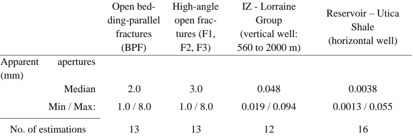
of faults Presence
Absence or open fractures parallel to one another
(lim-ited interconnection) Lithologies Faulting through high K rock Faulting through low K rocks
Fault plane properties Presence of some higher K units in the IZ Dominance of low K materi-als
Fault dips Steep dips and thus shorter pathways
Shallow dips and thus long-er pathways
Fault orientation with respect to maximum principal stresses
and its magnitude
Fault planes aligned with SHmax may be critically
stressed
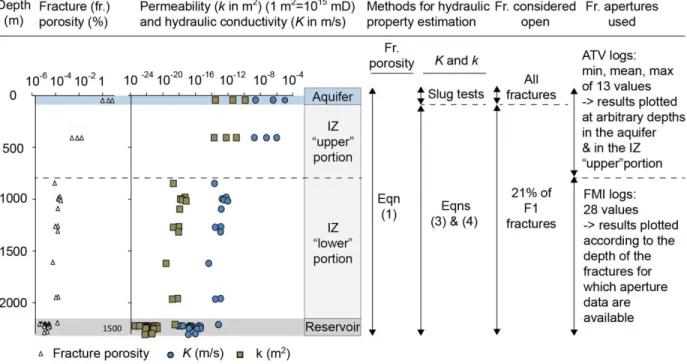
Fault planes orthogonal to SHmax are likely not critically
stressed
3.3.2 Specific analyses
377
Core and log data were analysed to assess the impact of clay shearing on the hydraulic behavior 378
of thrust faults. The shearing in clay-rich units (such as the shale-dominated succession of this 379
area) is indeed known to form clay gouge in fault planes (Weber et al. 1978; Lehner and Pilaar 380
1997; Sperrevik et al. 2000), which is generally considered a barrier to fluid flow (Yielding et al. 381
1997; Freeman et al. 1998). The presence and characteristics of fractures in the vicinity of thrust 382
faults was also documented and discussed here. 383
In addition, the fault core properties of a normal fault in the area (the Rivière Jacques-Cartier 384
fault zone) were assessed using the Shale Gouge Ratio (SGR) (Yielding et al. 1997; Freeman et 385
al. 1998). This widely used method is based on the estimation of the percentage of shale that has 386
slipped past a certain point along a fault. The latter is then used to estimate the fault seal capacity. 387
For comparison purposes, the empirical relationship of Sperrevik et al. (2002) was also used to 388
estimate the fault core properties. This relationship was developed to describe the observed corre-389
lation between clay content and permeability (k, in mD) at the scale of fault core samples 390
(Manzocchi et al. 1999; Sperrevik et al. 2002). This relationship also takes into account compac-391
tion and diagenesis effects, which strongly impact rock porosity and permeability and is particu-392
larly relevant for the study area. The reliability of this relationship was successfully tested in a 393
comparable geological context (Bense and Van Balen 2004). Details are provided in Appendix 2. 394
Fault seal analysis has been the focus of extensive recent studies (eg., Bense and Person, 2006) 395
and the SGR method is only one of them. This approach has been selected for the present study 396
because 1) the Sperrevik et al. (2002) method is based on field data from a comparable field geo-397
logical context to the sedimentary succession of the SLP, 2) this approach takes into account the 398
rock burial depth, which is a key parameter for rock permeability in the SLP and 3) it is also con-399
sistent with the approach successfully tested by Konstatinovskaya et al. (2012) using SGR in the 400
SLP. 401
4 Results
4.1 Hydraulic characterization of the fracture network
403
4.1.1 Open fracture properties
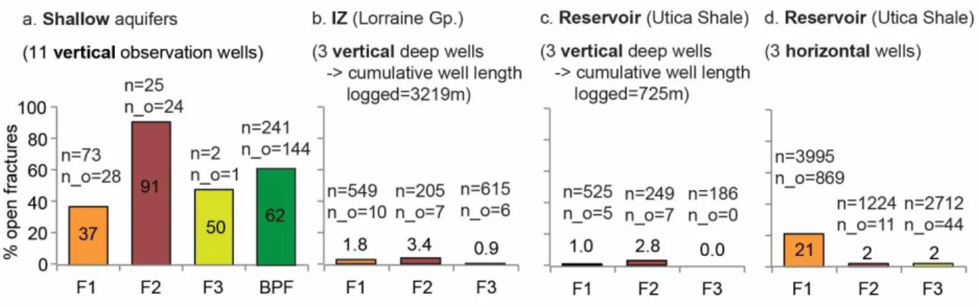
404
General trends and observations related to fracture apertures in the present dataset are as follow: 405
1) high proportions of open features were identified in the shallow aquifer in all fracture sets 406
(37%, 91% and 50% of the F1, F2 and F3 fractures, respectively) (Fig. 4a); 2) open bedding-407
parallel fractures (BPF) were only observed in shallow wells (Fig. 4a); 3) in the deep reservoir, a 408
higher proportion of open F1 fractures was encountered in the horizontal legs drilled in the Utica 409
Shale, compared with the F2 and F3 sets (21% of open F1 fracture versus 2% for F2 and F3 frac-410
tures) (Fig. 4d); 4) this higher proportion of open F1 fractures at depth was not observed in the 411
vertical wells drilled through the Utica Shale (Fig. 4c and d) nor in the IZ, but this is very likely 412
attributable to the fact that the high-angle fractures are significantly under-sampled in vertical 413
wells; 5) while approximately the same number of open fractures was identified in the IZ and gas 414
reservoir using the three vertical wells, this number was obtained for very different cumulative 415
well lengths: the segments logged in the reservoir were typically more than four times shorter 416
than in the IZ. Much more fractures were identified in the more brittle Utica Shale (Fig. 4b and 417
c), in agreement with previous observations by Ladevèze et al. (2018) considering all fractures 418
(see for instance Fig. 3). Therefore, lithology seemingly controls the number of open fractures. 419
Fig. 4 Percentage of open fractures from the total fracture population for the F1, F2, F3 and BPF
sets according to the data source; n: total number of fractures; n_o: number of open fractures; F1, F2 and F3: three high-angle fracture sets; IZ: Intermediate zone; BPF: bedding-parallel fractures; Gp.: Group.
As mentioned earlier, estimated apertures may be considered slightly overestimated since fracture 421
apertures are likely to be enhanced by drilling operations, especially in finely layered rocks such 422
as shales. This is particularly the case in the shallow aquifer where the rock decompaction further 423
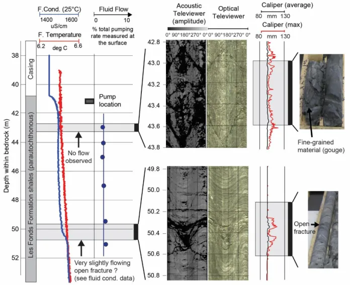
enhances this process. For this reason, some extreme aperture values (typically >10 mm) meas-424
ured at shallow depth using acoustic televiewer data (Crow and Ladevèze 2015) were excluded 425
from the analysis. Moreover, deep fracture apertures can also be slightly overestimated when 426
using FMI because of the limitations of the aperture estimation method (Davatzes and Hickman 427
2010). As a consequence, the fracture aperture values presented in Table 3 likely represent an 428
upper limit for realistic values in the study area. 429
Table 3 Available estimates for fracture apertures for the shallow and deep intervals.
430
Shallow wells Deep well B
Open bed-ding-parallel fractures (BPF) High-angle open frac-tures (F1, F2, F3) IZ - Lorraine Group (vertical well: 560 to 2000 m) Reservoir – Utica Shale (horizontal well) Apparent apertures (mm) Median 2.0 3.0 0.048 0.0038 Min / Max: 1.0 / 8.0 1.0 / 8.0 0.019 / 0.094 0.0013 / 0.055 No. of estimations 13 13 12 16
Shallow observation wells show an exponential decreasing trend of the open fracture density 431
within the upper 60 m of bedrock, with most of the open fractures being located in the first 30 m 432
(Fig. 5b, same trend for the two types of open features). There is no clear trend for the density 433
distribution of closed fractures with depth for the shallow observation wells (Fig. 5c). The dataset 434
for deep wells did not show any specific trend in the distribution of open fractures within the sed-435
imentary succession. 436
Fig. 5 Fracture density variations with depth within the bedrock in shallow wells. Data from 11
observation wells were combined. Fracture densities were calculated using a 5 m window length every 1 m. The number of wells according to the depth within the bedrock was used to
normal-ize fracture densities.
4.1.2 Assessment of the hydraulic properties throughout the succession
437
Fracture porosities, K and k values calculated for the shallow aquifer are presented in Figure 6 438
according to the depth at which aperture measurements are available (values presented in Appen-439
dix 3). The median fracture spacing values considered for the estimation of the number of open 440
fractures in the REV are respectively 0.2, 2.51, 0.11 and 0.17 m for the F1, F2, F3 and BPF frac-441
ture sets. Fracture aperture values used to calculate porosity come from Table 3. As the rock mass 442
of the shallow aquifer has open fractures that locally display some large apertures, the fracture 443
network significantly contributes to the total porosity of the rock mass (up to approximately 8%). 444
Hydraulic conductivities ranging from 2.3x10⁻⁹ to 1.1x10⁻⁵ m/s (with a median of 6x10⁻⁷ m/s) 445
were obtained from hydraulic tests performed in 11 shallow observation wells (less than 145 m 446
deep), all open to bedrock (Ladevèze et al. 2016). Higher K values were obtained in wells located 447
in the autochthonous domain, with a marked correlation associated with the presence of siltstone 448
interbeds. Wells in the parautochthonous domain intersect shale units that are highly folded and 449
faulted and display lower K values. These values suggest the presence of significant fluid flow 450
circulation at shallow depth in the fractured shale-dominated aquifer, mainly through open BPF 451
that are connected to open sub-vertical fractures. Figure 6 also presents fracture porosities, K and 452
k values calculated for the IZ and reservoir with Eqns 3 and 4 using the fracture aperture esti-453
mates provided in Table 3 (values available in Appendix 3). The median fracture spacing value 454
considered for the estimation of the number of open F1 fractures in the REV is 0.14 m (measured 455
in horizontal sections of deep wells, see Ladevèze et al. (2018) for more details). 456
Contrary to those in the shallow units, deeper open fractures only slightly contribute to the total 457
porosity. Pores of the rock matrix are then the most significant contributors to total porosity, as 458
the latter was reported having a median value of 3.3% for the Lorraine Group and the Utica Shale 459
based on laboratory and log analyses on core samples (BAPE 2010; Nowamooz et al. 2013; 460
Séjourné et al. 2013; Séjourné 2015). Extremely low values of K and k for the deep fracture net-461
work were thus obtained using the cubic law and the apertures estimated in both the lower por-462
tion of the IZ and in the reservoir. Nonetheless, these geometric mean k values (10-18 to 10-24 m2) 463
are within the range of matrix permeabilities proposed in the literature for the deep units of the 464
Lorraine Group and Utica Shale: geometric mean values around 10-20 m2, with extreme values 465
ranging from 10-16 to 10-27 m2 (BAPE 2010; Séjourné et al. 2013). When considering the fracture 466
apertures estimated in the shallow aquifer for F1 fractures, values of k around 10-13 m2 are ob-467
tained, which are close to the upper limit of the range reported for the deeper units. 468
No clear trend with depth of the hydraulic properties was identified in the lower portion of the IZ 469
and in the reservoir (Fig. 6). However, when comparing the values estimated in each of the geo-470
logical intervals (shallow aquifer, upper portion and lower portion of the IZ and reservoir), there 471
is a global decreasing trend for these values with depth. As such, only limited fluid circulation 472
can be envisioned in the lower portion of the IZ and in the reservoir. 473
Fig. 6 Variation with depth of the estimated fracture porosities, hydraulic conductivity (K) and
corresponding permeabilities (k). K values from slug tests (field data) were initially presented in Ladevèze et al., 2016. ATV: Acoustic Televiewer; FMI: Formation Micro Imager; IZ: Interme-diate Zone. Numerical values are presented in Appendix 3.
475
4.2 Hydraulic characterization of fault zones
476
4.2.1 Fault zone architecture
477
The autochthonous domain of the SLP hosts some isolated and steeply dipping normal faults, 478
such as the Rivière Jacques-Cartier fault (Fig. 1). Their steep dips combined with the overall 479
thinning of the sedimentary succession and the shallowing of the platform towards the northwest 480
would provide the shortest and most direct pathways between the Utica Shale and fresh water 481
aquifers. This geometry contrasts with the parautochthonous and allochthonous domains to the 482
southeast, where shallow-dipping regional thrust faults propagate from southeast to northwest 483
(Fig. 1), often displaying an imbricated fan geometry (St-Julien et al. 1983; Séjourné et al. 2003; 484
Castonguay et al. 2006). 485
Therefore, potential pathways in thrust faults of the study area would have to develop over much 486
longer distances than in normal faults, not only because the Utica Shale is much deeper than in 487
the northern part of the study area, but also due to the much more complex geometry associated 488
to the thrust faults. 489
4.2.2 Thrust fault zone
490
Fine-grained rocks were observed in fault planes identified in a few core samples (Erreur ! 491
Source du renvoi introuvable.) from shallow wells; they are here called “gouge”, as proposed
492
by Sibson (1977). Gouge was also observed in the thrust fault planes of the parautochthonous 493
domain on optical logs of a few shallow observation wells. The presence of this gouge may have 494
caused the sealing of the fault core, which would thus constitute a barrier to fluid flow. Heat-495
pulse flowmeter tests performed in several shallow observation wells (Crow and Ladevèze 2015) 496
confirmed that little to no flow occur in the presence of these thrust fault planes. This is also con-497
sistent with the low hydraulic conductivity values calculated in shallow wells of this area, which 498
displays significant faulting/folding evidence that is characteristic of the parautochthonous do-499
main (Ladevèze et al. 2016). Nonetheless, the presence of a few open fractures was also noted in 500
some of these logs and can probably explain the presence of local shallow fluid flow circulation 501
(see for instance the slight variation in the fluid conductivity log in the vicinity of an open frac-502
ture in Erreur ! Source du renvoi introuvable.). 503
Fig. 7 Examples of results obtained from borehole geophysical logging (Crow and Ladevèze
2015) performed in a 50 m observation well drilled in the parautochthonous domain within the thrust sheet domain, showing intervals with noticeable faulting and folding, along with open fractures.
504
Data from deep shale gas well logs indicate that open fracture densities associated with thrust 505
planes were higher in the vicinity of the Appalachian structural front (see Appendix 4 showing 506
higher values for well A). This finding is in agreement with previous observations when consid-507
ering fractures without considering their aperture (Séjourné 2015; Ladevèze et al. 2018). None-508
theless, open fracture density values obtained in the deep shale gas wells remain significantly 509
lower than those calculated in the shallow observation wells (see values in Fig. 5). 510
These preliminary observations suggest that there is a possible correlation between open fracture 511
density and the presence of faults. To confirm this potential relationship, a more detailed compar-512
ison of open fracture density variation with fault proximity was undertaken at the borehole scale 513
using FMI data from the horizontal leg of well A, where a fault zone can be observed. In well A, 514
the fault zone is within the Utica Shale and consists of a highly fractured damage zone that sur-515
rounds two fault planes that are dipping toward the NW at about 25° (the two planes are closely 516
spaced, so to simplify the analysis, only one plane is hereafter considered) (Ladevèze et al. 2018). 517
In this section of well A, almost all the open fractures have the same orientation as F1 fractures 518
(95 % of the open fractures in the horizontal portion of well A). 519
The open fracture density globally decreases with increasing perpendicular distance from the 520
fault zone (Erreur ! Source du renvoi introuvable.). The open fracture distribution is clearly 521
not continuous along the horizontal portion of the well, but rather show clusters. Figure 8b shows 522
that in well A, three fracture clusters are separated by distances of approximately 80 to 135 m. As 523
proposed in Ladevèze et al. (2018), F1 fractures are likely concentrated in corridors, although this 524
pattern remains to be confirmed. Therefore, this suggests that these open fractures probably be-525
long to the F1 set, although the possibility of the existence of a new fracture set associated with 526
these fault zones cannot currently be dismissed. 527
Fig. 8 Open fracture density variation in the vicinity of a fault plane in the horizontal section of
well A: a. conceptual diagram illustrating the difference between the distance perpendicular to the fault and the distance along the horizontal section of the well (used to estimate the possible relationship between fracture density and fault proximity). The angle α represents the angle be-tween the fault plane and the borehole direction; b. density variations of open F1 fractures with respect to the distance from a fault zone in the horizontal portion of well A. Fracture densities were corrected for sampling bias using the Terzaghi (1965) method.
4.2.3 Normal fault zone
529
In the SLP, the high angle (near vertical) NE-SW faults (normal faults) oblique to SHmax are more
530
likely to be reactivated (Konstantinovskaya et al. 2012). Therefore, these normal faults are likely 531
critically stressed and potentially hydraulically active. However, this hypothesis would need to be 532
addressed more in details, but a thorough study of the hydro-mechanical attributes of the Rivière 533
Jacques-Cartier fault to further assess the impact of the fault reactivation on its hydraulic proper-534
ties is beyond the scope of the paper. 535
To the south-west of the study area, observations from at least two deep wells have shown that 536
gouge forms in normal faults of the SLP (wells A027 and A125 in the Bécancour area; see 537
Séjourné et al., 2013). Clay-rich shales were also suspected to have been displaced along the Ri-538
vière Jacques-Cartier normal fault. Because the stratigraphic units that are cut by normal faults 539
(shales from the Lorraine Group) contain a significant proportion of clay, the term “clay gouge” 540
(Vrolijk et al. 2016) is used hereafter. 541
In this area, the calculated SGR values decrease progressively with increasing depth (Fig. Er-542
reur ! Source du renvoi introuvable.) since the volume of shale (Vsh) also decreases progres-543
sively with increasing depth in the sedimentary succession (shale-dominated to carbonate-544
dominated units). SGR values over 20% (interpreted as sealed structures according to (Yielding 545
et al. 1997)) were calculated for the segments of the normal fault above the Utica Shale reservoir 546
(Fig. Erreur ! Source du renvoi introuvable.); this value suggests the presence of clay gouge in 547
these segments and, hence, a sealing behavior. These preliminary results are in agreement with a 548
similar analysis carried out for the Yamaska fault to the south-west of the study area 549
(Konstantinovskaya et al. 2014b). Moreover, in both regions, lower SGR values were found in 550
carbonate-dominated units below the Utica Shale, suggesting a slightly more permeable medium. 551
With the Sperrevik et al. (2002) equation, k values range approximately from 10-21 to 10-24 m2 552
and 10-24 to 10-26 m2 respectively for the core of theoretical Fault 1 and 2 in Figure. Erreur ! 553
Source du renvoi introuvable.. These values are either similar to or lower than those obtained
554
for the fracture network at depth using the cubic law relationship (see Fig. 6). Although not con-555
sidered precise, these semi-quantitative estimates confirm that permeability values of the normal 556
fault core is likely extremely low. These results also advocate for significant sealing behavior of 557
the fault core in the IZ, impeding flow across it. Moreover, this analysis highlights the crucial 558
need for field data, including in situ permeability tests or pressure gradient estimations across a 559
fault zone, to better calibrate these empirical relations and to more accurately determine the hy-560
draulic behavior of the fault gouge. 561
562
Fig. 9 Cross-section of the Rivière Jacques-Cartier fault system (see location in Fig. 1) used for
the Shale Gouge Ratio (SGR), permeability (k) (expressed in m2; 1 m2=1015 mD) and hydraulic conductivity (K) calculations along the fault planes of the Rivière Jacques-Cartier fault. T: fault true displacement; Δz: thicknesses of the stratigraphic units; Vsh: volume of shale.
5 Discussion
563
5.1 Hydraulic behavior of open fractures
564
Based on the open fracture distribution in the shallow fractured rock aquifer, IZ and reservoir, 565
two hydrogeological domains were defined. The first corresponds to the shallowest portion of the 566
bedrock where most of the flow is concentrated (active flow zone). The second hydrogeological 567
domain corresponds to the IZ and reservoir (deep intervals) where very little flow takes place. 568
Most of the open fractures are concentrated in the upper 30 to 60 m of bedrock, although some 569
open fractures were also locally observed down to 145 m in the deepest observation well of the 570
study area (Crow and Ladevèze 2015). However, as this well displays particularly low K values 571
(±10-9 m/s) compared to the other observation wells, these fractures seemed to be nearly hydrau-572
lically inactive (Ladevèze et al. 2016). Thus, an arbitrary limit of 60 m within bedrock is pro-573
posed here to delimit the two hydrogeological domains, but it must be kept in mind that this 574
boundary is gradual and could certainly be spatially variable. Nonetheless, geochemical profiles 575
performed in four of the shallow observation wells (drilled between 15 to 145 m within the shal-576
low fractured rock aquifer) indicated that water types changed from CaHCO3 or NaHCO3
(corre-577
sponding to relatively recent water) in the upper part of the wells, to NaCl at the bottom (corre-578
sponding to evolved water with much longer residence time) (Bordeleau et al. 2018b), thereby 579
providing additional evidence for the lower limit of the shallow groundwater active zone. 580
5.1.1 In the shallow rock aquifer
581
In the shallow rock aquifer (0-60 m within bedrock), there is a high proportion of open fractures, 582
both sub-vertical and sub-horizontal, which have apertures larger than 1 mm. This high propor-583
tion of “large” open fractures plays a significant role for groundwater circulation, especially 584
where open BPF are interconnected with sub-vertical open fractures. The decreasing density of 585
open BPF within the first 60 m is likely to be related to the increase of the stress normal to BPF 586
planes as a consequence of the increase of the overburden stress with depth. The degree of con-587
nectivity of open fractures, and thus fluid circulation, is thus limited as depth increases. 588
The NW striking F2 fracture set seems preferentially open (91% of F2 fractures). The preferential 589
fying fracture orientations using shallow well log data and their number was limited (25). The 591
other facture sets also display significant proportions of open fractures (37% of F1 fractures and 592
50% of F3 fractures). Thus, in shallow wells, the orientation is not a critical factor for fracture 593
opening as total stresses tend to be equal at shallow depth. This finding contrasts with the state-594
ment that open fractures (and thus the anisotropic permeability tensor) should be preferentially 595
oriented parallel to the orientation of the present-day maximum horizontal stress (SHmax) in
shal-596
low aquifers (Mortimer et al. 2011). In fact, SHmax is oriented NE-SW in this region
597
(Konstantinovskaya et al. 2012), parallel to the orientation of the F1 fractures. The probable ex-598
planation is that previously closed fractures could have been re-opened under the influence of 599
post-glacial surface processes. It is indeed recognized that episodes of glaciation and de-600
glaciation can enhance the opening of pre-existing fractures at shallow depths (Wladis et al. 601
1997; Martini et al. 1998). These effects, combined with decompaction in a context of erosion 602
and uplift, could likely explain the opening of fractures at shallow depths regardless of their ori-603
entation. 604
5.1.2 In the deep intervals (intermediate zone and reservoir)
605
The situation is different below this circa 60 m threshold, as most of the open fractures observed 606
are sub-vertical, essentially belonging to the F1 fracture set. F1 fractures are parallel to the con-607
temporary NE-SW orientation of SHmax, thereby in agreement with the theory proposed by Barton
608
et al. (1995) stating that the contemporary in situ stress regime at depth should preferentially con-609
trol the opening of fractures that are aligned with SHmax. It must also be noted that overpressured
610
conditions were identified in the Utica Shale and at the base of the Lorraine Group (Morin 1991; 611
BAPE 2010; Chatellier et al. 2013) could also be responsible for the presence of these open frac-612
tures. However, because the dissolution of fracture fillings may contribute to the presence of 613
open fractures whatever their orientation (Laubach 2003; Laubach et al. 2004), the existence of 614
open fractures from the F2 and F3 sets cannot be discarded. Nonetheless, few observations of 615
such features were made in well logs. For this reason, it is concluded that the in situ stress regime 616
is the dominant cause for fracture opening at depth. 617
Bedding-parallel fractures were not specifically observed in the available shale gas well logs, but 618
were documented by a few authors in other shale gas plays (Rodrigues et al. 2009; Gale et al. 619
2015). Because of the overburden pressure on the sedimentary succession, the BPF should be 620
closed at depth in spite of overpressured conditions documented in deep hydrocarbon exploration 621
wells identified in the Utica Shale and at the base of the Lorraine Group. Hence, these structures 622
are not considered conductive for fluid flow. 623
A fluid flow model of this study area should thus take into account the fact that the hydraulic 624
conductivity (K) would likely be anisotropic, with a preferential orientation according to the F1 625
fracture strike. Moreover, as the fractures are rotated according to bedding plane orientations 626
(Ladevèze et al. 2018), the K tensor should follow these bedding plane orientations, as proposed 627
in the work of Borghi et al. (2015). 628
The proposed analysis of the contribution of open fractures to fluid circulation at depth was car-629
ried out using analytical solutions based on theoretical assumptions and limited available datasets 630
of fracture apertures and open fracture distribution in rock mass. Therefore, the calculated values 631
must be considered with caution. Also, the method based on the cubic law has been challenged 632
for fractures displaying low aperture values (less than 0.004 mm, which is the case here when 633
considering fracture apertures from the reservoir) (Witherspoon et al. 1980). Furthermore, these 634
calculations are based on the assumption of a laminar flow between two parallel fracture planes. 635
This assumption can lead to significant errors, as it is now documented that the geometry of the 636