High resolution mapping of ice mass loss
in the Gulf of Alaska from constrained
forward modelling of GRACE data
CHEICK DOUMBIA1*, PASCAL CASTELLAZZI2, Alain N. Rousseau1, Macarena Amaya3
1Institut National de la Recherche Scientifique (INRS), Canada, 2Deep Earth Imaging, Commonwealth Scientific and Industrial Research Organisation, Australia, 3Faculty of Astronomical and Geophysical Sciences, National University of La Plata, Argentina
Submitted to Journal: Frontiers in Earth Science Specialty Section: Cryospheric Sciences Article type:
Original Research Article Manuscript ID: 487671 Received on: 27 Jul 2019 Revised on: 10 Dec 2019
Frontiers website link:
www.frontiersin.org
The authors declare that the research was conducted in the absence of any commercial or financial relationships that could be construed as a potential conflict of interest
Author contribution statement
Cheick Doumbia performed the data analysis and wrote the manuscript. Pascal Castellazzi trained the first authors to process GRACE data, verified the results, and contributed in writing the manuscript. Alain N. Rousseau designed and led the project, supervised the first author, and contributed in writing the manuscript. Macarena Amaya helped in building a comprehensive literature review on the topic.
Keywords
glaciers, ice melt, GRACE (Gravity recovery and climate experiment), Forward modelling, Gulf of Alaska
Abstract
Word count: 270
The resolution of GRACE Terrestrial Water Storage change data is too low to discriminate mass variations at the scale of glaciers, small ensemble of glaciers, or icefields. In this paper, we applied an iterative constraint modelling strategy over the Gulf of Alaska (GOA) to improve the resolution of ice loss estimates derived from GRACE. We assess the effect of the most influential parameters such as the type of GRACE Level-2 solution and the degree of heterogeneity of the distribution map over which the GRACE data is focused. Three GRACE solutions from the most common processing strategies and three ice distribution maps of resolutions ranging from 55,000 km2 to 20,000 km2 are used. First, we present results from a series of simulations with synthetic data or a mix of synthetic/modelled data to validate the focusing strategy and we point out how inaccuracies arise while increasing the spatial resolution of GRACE data. Second, we present the recovery of the total GRACE-derived mass change anomaly at the scale of the GOA. At this scale, all solutions and distribution maps agree, showing ~40 Gt/yr of mean ice mass loss over the 2002-2017 period. This result is similar to studies using GRACE solutions from the latest releases and time-series of more than 8 years. The first studies using GRACE data published during the 2005-2008 era generally overestimated the total ice mass loss. Third, we show results of the three resolutions tested to focus the mass anomaly. Using focusing units (mascon) of ~30,000 km2 or larger, the focusing procedure provides reliable results with errors below 15%. Below this threshold, errors of up to 56% are observed.
Contribution to the field
This paper presents how low-resolution time-variable gravity data can be downscaled to better understand ice mass loss at the regional scale. In the Gulf Of Alaska, a large-scale signal of mass loss, extending over a ~1500-km-long stretch, is observed by the two satellites of a well-known gravity recovery mission (GRACE). This anomaly corresponds to ice mass loss from numerous glaciers located along the southern coast of Alaska (USA) and Yukon (Canada). While the total mass can be recovered using GRACE data, the resolution of such observation is too low to derive ice mass loss at the scale of glaciers, ice fields, or at the regional scale. We present how, using a distribution map of the glaciers, GRACE signal can be focused to smaller spatial units. More importantly, we explore the limits of the procedure: while the processing strategy chosen to process GRACE data is not important when interpreting the signal at the scale of the anomaly, it becomes an important parameters while trying to discriminate its small-scale contributors.
Funding statement
The authors wish to gratefully acknowledge the financial support of the Natural Sciences and Engineering Research Council of Canada (NSERC) and the Yukon Energy Corporation (YEC) for this research.
Studies involving animal subjects
Generated Statement: No animal studies are presented in this manuscript.
Studies involving human subjects
Generated Statement: No human studies are presented in this manuscript.
Inclusion of identifiable human data
Generated Statement: No potentially identifiable human images or data is presented in this study.
constrained forward modelling of GRACE data
2 3
Cheick Doumbia1*, Pascal Castellazzi2, Alain N. Rousseau1, Macarena Amaya3
4 5
1 Institut national de la recherche scientifique (INRS), Centre Eau Terre Environnement, 6
Université du Québec, 490 rue de la Couronne, Québec, QC, Canada, G1K 9A9. 7
8
2 Commonwealth Science and Industrial Research Organisation (CSIRO), Land and Water, 9
Waite Rd, Urrbrae SA 5064, Australia 10
11
3 Facultad de Ciencias Astronómicas y Geofísicas, Universidad Nacional de La Plata (UNLP), 12
Paseo del Bosque s/n, B1900FWA La Plata, Buenos Aires, Argentina 13 14 * Correspondence: 15 Cheick Doumbia 16 [email protected] 17
In review
2 This is a provisional file, not the final typeset article
Keywords: Glaciers1, ice melt2, GRACE3, Forward modelling4, Gulf of Alaska5
18 19
Abstract
20
The resolution of GRACE Terrestrial Water Storage change data is too low to discriminate mass 21
variations at the scale of glaciers, small ensemble of glaciers, or icefields. In this paper, we apply 22
an iterative constraint modelling strategy over the Gulf of Alaska (GOA) to improve the resolution 23
of ice loss estimates derived from GRACE. We assess the effect of the most influential parameters 24
such as the type of GRACE solution and the degree of heterogeneity of the distribution map over 25
which the GRACE data is focused. Three GRACE solutions from the most common processing 26
strategies and three ice distribution maps of resolutions ranging from 55,000 km2 to 20,000 km2 27
are used. First, we present results from a series of simulations with synthetic data or a mix of 28
synthetic/modelled data to validate the focusing strategy and we point out how inaccuracies arise 29
while increasing the spatial resolution of GRACE data. Second, we present the recovery of the 30
total GRACE-derived mass change anomaly at the scale of the GOA. At this scale, all solutions 31
and distribution maps agree, showing ~40 Gt/yr of mean ice mass loss over the period 2002-2017. 32
This result is similar to studies using GRACE solutions from the latest releases and time-series of 33
more than 8 years. The first studies using GRACE data published during the 2005-2008 era 34
generally overestimated the total ice mass loss. Third, we show results of the three resolutions 35
tested to focus the mass anomaly. Using focusing units (mascon) of ~30,000 km2 or larger, the 36
focusing procedure provides reliable results with errors below 15%. Below this threshold, errors 37
of up to 56% are observed. 38
39
3 This is a provisional file, not the final typeset article
Introduction 40
Glaciers represent 68.9% of fresh water resources worldwide. In different regions of the world, 41
people rely on glacier meltwater for agriculture, hydropower, industries and municipal water 42
requirements (Chen and Ohmura 1990; Blanchon and Boissière 2009). However, over the last 43
decades, the glacier mass losses have raised concerns in and beyond the research communities. 44
Climate change leads to important reductions in glacial water storage. Glaciers have an important 45
influence on sea level rise; hence their melt threatens the living environment of costal dwellings. 46
Jin and Feng (2016) estimated the contribution of glacial melt to sea level change between 2003 47
and 2012 at 1.94 ±0.29 mm/yr. From 120,000 glaciers available in the World Glacier Inventory, 48
Radić and Hock (2011) estimated that the total volume loss could be as much as 21 ±6% by 2100, 49
leading to a total sea level rise of 124 ±37 mm. 50
Numerous studies focused on estimating the ice mass loss over specific continents, regions, or 51
Mountain ranges. For example, Larsen et al. (2007) investigated glacier changes in southeast 52
Alaska and northwest British Columbia over the period 1948-2000 and 1982/1987-2000, 53
respectively. By combining the results from these periods, they estimated an average ice mass loss 54
rate of around 15.03 ±4 Gt/yr (considering an ice density of 900 kg/m3). In the Canadian Rocky 55
Mountains, Castellazzi et al. (2019) estimated a total of 43 Gt/yr of glacial mass loss over the 56
period 2002-2015. Over the entire Gulf of Alaska area, Gardner et al. (2013) found 50 ±17 Gt/yr 57
of glacial melt by using spaceborne altimetry data (e.g. ICESat) over the period 2003-2009. 58
Berthier et al. (2010) obtained 37.47 ±8 Gt/yr of glacier ice loss from Digital Elevation Models 59
(DEM) for the period 1962-2006. Larsen et al. (2015) used airborne altimetry to estimate glacier 60
mass loss rate over the period 1994–2013 and found 75 ±11 Gt/yr. 61
Gravity data provides direct information over ice mass changes, as the link between gravity and 62
mass is direct and requires no calibration. In situ gravity measurements are labour-intensive, costly 63
to acquire and point-based; while satellite gravity data are limited in resolution due to the sensing 64
distance. Since 2002, the USA (NASA) and the German (DLR) space agencies have led the 65
GRACE mission (Gravity Recovery and Climate Experiment). It aims at monitoring the variations 66
of the Earth’s gravity field with a temporal resolution of a few days to a month, with a spatial 67
resolution of ±400 km (Tapley et al. 2004; Ramillien et al. 2017). The variations in the Earth's 68
mass distribution causes changes in the gravity field (Wahr et al. 1998). Thus, by mapping the 69
variations of the gravitational field, GRACE assesses the Earth’s mass distributions. The mass 70
redistribution obtained from GRACE data, contains changes in Terrestrial Water Storage (TWS), 71
and oceanic mass (Wahr et al. 1998; Chen et al. 2006). Yirdaw et al. (2009) noted the GRACE 72
mission estimates could be used to monitor the rate of change of TWS over large spatial scales. 73
Ramillien et al. (2017) further stressed that continental hydrology is one of the main applications 74
of GRACE data. The variation of TWS aggregates changes in surface water, soil moisture, ground 75
water, snow and ice. Jin and Zou (2015) used GRACE data to estimate a high-precision glacier 76
mass dynamics in Greenland. In the Gulf of Alaska (GOA) region, GRACE data have been used 77
in different studies to estimate glacier mass loss (Tamisiea et al. 2005; Chen et al. 2006; Arendt et 78
al. 2008; Luthcke et al. 2008; Arendt et al. 2009; Arendt et al. 2013; Baur et al. 2013; Beamer et 79
al. 2016; Wahr et al. 2016; Jin et al. 2017). 80
Two main types of GRACE Level-3 solutions are used in hydrological applications. There are 81
unconstrained solutions, relying on de-stripping and spherical harmonics truncation, and 82
constrained solutions often relying on regularization or stabilization. Among the later, mascon 83
solutions, obtained after inverting the GRACE signal into a mass change for each spatial unit 84
(‘mascon’) of a predefined grid, have become particularly popular over the last years (e.g. Save et 85
4 This is a provisional file, not the final typeset article
al. 2016). Meanwhile, the unconstrained GRACE spherical harmonics solutions present errors at 86
high spatial frequencies (e.g. N˃60 or 300 km) and North-South stripes mainly due to gravitational 87
model corrections, instrument errors, and gaps in data coverage. Destriping, truncation and 88
filtering are usually applied on these Level-2 solutions to reduce high frequency errors and to 89
eliminate stripes. The challenge of using GRACE data to investigate hydrological fluxes, such as 90
mass variations at the glacier-scale, lies in the low spatial resolution (300/400 km) and the inability 91
to discriminate close masses. Leakage effects are inherent to the GRACE sensing strategy, and is 92
accentuated by the truncation and filtering used to ‘clean’ the monthly gridded mass changes. This 93
makes GRACE prone to large errors when considering areas below 200,000 km2 (e.g. 94
Longuevergne et al. 2010). To overcome this problem, several authors combined GRACE data 95
with other sources of information (e.g Castellazzi et al. 2018, 2019). 96
Different strategies such as scaling approach, additive approach, multiplicative approach and 97
unconstrained or constrained forward modelling approaches permit to partially restore the signal 98
loss (Long et al. 2016). A constrained inversion method can also be applied to improve the spatial 99
resolution of GRACE data (Farinotti et al. 2015; Long et al. 2016; Castellazzi et al. 2018). Chen 100
et al. (2015) used forward modelling to restore the GRACE signal amplitude of Antarctic ice and 101
glacier loss due to the noise reduction. Long et al. (2016) showed that a constrained forward 102
modelling can spatially recover the distribution details of the GRACE signal. Farinotti et al. (2015) 103
estimated the glacier mass loss in the Tien Shan (China) by subtracting the non-glacier 104
contributions from the total mass change. They used an inversion method with a priori information 105
about the glacier spatial distribution in area subdivisions (i.e. mascon and sub-mascon). By 106
improving GRACE spatial resolution, their results are comparable to those derived from altimetry 107
data and glacial melt modelling (e.g. the Cold Regions Hydrological Model - Pomeroy et al., 2007 108
- and the Distributed Enhanced Temperature Index Model - Hock, 1999). Studying groundwater 109
depletion in Central Mexico, Castellazzi et al. (2016, 2018) improved the GRACE spatial 110
resolution using InSAR-derived ground-displacement maps to constrain the forward model. They 111
subtracted groundwater contributions from other components of TWS, built a distribution map of 112
groundwater depletion using InSAR, and focused GRACE data over it. The potential of separating 113
masses depends on the size, separation, and amplitude of the masses, as well as on the available 114
constraining data and their efficiency in explaining the low resolution GRACE signal. 115
Although several authors have injected ancillary data into GRACE post-processing to improve the 116
resolution, there is still a need to assess how constrained modelling improves the interpretation of 117
GRACE data versus simplistic approaches such as spatial averaging (e.g. usually over watersheds 118
or regions). While few studies already tested how constrained forward model can help interpreting 119
GRACE data, case studies are still lacking and more importantly, the limits of the procedure are 120
still relatively unknown. In this study, we apply this procedure to build a high-resolution ice mass 121
loss map from GRACE data over a large range of melting glaciers in the GOA. In that perspective, 122
we use several GRACE solutions, apply a spatial constraint to focus the signal and provide a high-123
spatial resolution map of ice mass loss over the study area. 124
125
Study area 126
Our study area is delimited by zone 10 (Fig. 1). The area was selected to cover the glaciers of the 127
GOA and to include a stretch of ~300 km of the surroundings to account for spatial leakages 128
inherent to the GRACE signal. During the last decade, different studies used GRACE data to 129
estimate glacier mass across the same region (Fig. 1). 130
5 This is a provisional file, not the final typeset article
There are discrepancies in mass losses estimated over the GOA. Most authors obtain values 131
ranging from -47 to -110 Gt/yr of glacial mass change (Fig. 1; Table 1). These studies consider 132
different spatial extents and data time-periods. For example, the total surface coverage considered 133
by Tamisiea et al. (2005) is 701,000 km², while Beamer et al. (2016) consider 420.300 km². The 134
first three studies show higher values of mass loss (Tamisiea et al. 2005; Chen et al. 2006; Luthcke 135
et al. 2008) than those more recent (Baur et al. 2013; Beamer et al. 2016; Wahr et al. 2016; Jin et 136
al. 2017). It is potentially due to the relatively short GRACE time-series available at that time and 137
the higher uncertainties in the earlier releases of GRACE data. In addition, variations in the 138
GRACE data processing strategy, including levels of filtering and spherical harmonic truncation, 139
might also contribute to discrepancies between studies. For example, some studies used 140
unconstrained solutions (Tamisiea et al. 2005; Chen et al. 2006; Baur et al. 2013; Jin et al. 141
2017). Other authors used mascon solutions at different spatial and temporal resolutions (Arendt 142
et al. 2008, 2009, 2013; Luthcke et al. 2008, 2013; Jacob et al. 2012; Beamer et al. 2016; Wahr et 143
al. 2016). Tamisiea et al. (2005) used unconstrained solutions completed up to Spherical 144
Harmonics (SH) degree and order 70. Other authors used SH degree and order up to 60 (Chen et 145
al. 2006; Baur et al. 2013; Jin et al. 2017). Jin et al. (2017) applied a Gaussian filter with a radius 146
of 300 km while the aforementioned studies used a radius of 500 km. Using a scaling factor 147
approach, Tamisiea et al. (2005) reduced the GRACE signal attenuation and leakage. A forward 148
modelling approach was also used by several authors to restore signal leakages from coastal 149
glaciers to the ocean (Baur et al. 2013; Jin et al. 2017). 150
Some authors also used auxiliary data to complement GRACE observations. Remote sensing of 151
ice surface elevation (e.g. ICESat NASA, airborne laser altimetry) was combined with GRACE 152
data (Arendt et al. 2008, 2013; Jin et al. 2017). Meteorological models also contributed to GRACE 153
science (Arendt et al. 2009; Wahr et al. 2016). Some authors combined remote sensing and 154
meteorological data to enrich and validate glacier mass loss estimates (Arendt et al. 2013; Luthcke 155
et al. 2013). Beamer et al. (2016) developed hydrological models and compared their results with 156
the airborne altimetry and GRACE data. 157
158
Data and Methods 159
3.1. Glacier data and mascon delineation
160
Glaciers are delimited using the GLIMS Glacier Database released on 27/10/2017 and available 161
online (http://nsidc.org/glims/; GLIMS and NSIDC 2005, updated in 2013). It is a continuation of 162
the World Glacier Inventory (Raup et al. 2007) which compiles different sources: satellite imagery 163
data, historical information from maps, and aerial photography. Recently, the GLIMS glacier 164
Database was merged with the Randolph Glacier Inventory (RGI). This combination was 165
performed to support the fifth report of the Intergovernmental Panel on Climate Change (Pfeffer 166
et al. 2014). While the GLIMS database may contain errors, it is, at least for our study area, in 167
good agreement with the glacier inventory of Alaska and northwest Canada proposed by Kienholz 168
et al. (2015). According to GLIMS, the total glacier cover in the GOA area was around 90,000 169
km2 in 2013 (Fig. 2). 170
To ease data handling and make this dataset compatible with other GRACE grids used in this 171
study, the glacier distribution was resampled to a 0.25° grid (~28 km by ~14 km pixels; Fig. 2). 172
The resampling is performed using the following steps: (1) creation of a global 0.25-degree raster; 173
(2) overlay of the glacier footprint (taken as polygons) from the GLIMS data on the raster; (3) 174
creation of the distribution map. In the latter step, we consider that a pixel from step (1) contain 175
glacial masses if its center is within a glacier polygon from GLIMS. 176
6 This is a provisional file, not the final typeset article
Separating the contribution from a set of small masses to a low resolution signal (such as GRACE) 177
can be challenging and the success relies principally on the initial resolution, the final resolution, 178
the size of the masses, the distance separating them, and the amplitude of the changes for each 179
mass. Their spatial separation is important, close masses being harder to discriminate than those 180
spatially distant. To test the separation of the signal into a set of contributing masses, we considered 181
three different spatial distributions of mass at different resolutions (Table 2). Each area delimiting 182
a mass is referred to as a mascon (mass concentration area). 183
The GOA glaciers mass losses are spatially heterogeneous due to the difference in size of glaciers, 184
local hypsometry and climate (i.e. temperature and precipitation; Huss and Hock 2018; Frans et 185
al. 2018). For simplification, we assumed a uniform distribution of ice mass loss within each 186
mascon and test this assumption through a synthetic test (section 3.4). This assumption has been 187
used in other areas prone to ice mass loss by Chen et al. (2009) and in Farinotti et al. (2015). 188
189
3.2. GRACE TWS data
190
Three versions of Level-3 GRACE data in Water Thickness Equivalent (WTE) are considered. 191
The first solution is the stabilized solution from the Space Geodesy Research Group (GRGS RL04 192
- http://grgs.obs-mip.fr/grace) available at Spherical Harmonics (SH) degree and order 90. The 193
second is an unconstrained solution from the Center for Space Research (CSR RL06) complete up 194
to Spherical Harmonics (SH) degree and order 96 and de-striped/filtered in a single step by 195
applying the DDK8 filter (Kusche 2007; Kusche et al. 2009). The third is the CSR RL05 196
regularized Mascon solution from Save et al. (2016). All solutions are truncated up to Spherical 197
Harmonics (SH) degree and order 90 to better perceive the differences in the data processing 198
strategies without being influenced by the differences in resolution. The solutions are referred to 199
as GRGS, T96DDK8 and CSR-MASC hereafter. These solutions follow different processing 200
protocols and assumptions; hence we consider that their discrepancy represent an estimation of the 201
impact of the choice of the processing strategy. They comprise 150, 156 and 159 near-monthly 202
measurements, respectively, extending from 2002 to 2017. For consistency, the land mask applied 203
to produce the CSR-MASC solution (Save et al. 2016) is applied to all trend maps. All processing 204
is performed over the same 0.25° grid. 205
2D trend maps are derived from the three near-monthly solutions. The trend is computed by 206
subtracting an iteratively fitted sine curve of 1-year period. A 13-month moving average is then 207
applied to smooth out the residual. These steps contribute to remove the seasonal variations and 208
prevent contamination of trend estimates by seasonal signals. Finally, for each pixel, the slope of 209
a fitted linear curve is interpreted as the mass change rate. 210
Glacial Isostatic Adjustment (GIA) influences over the TWS trend need to be removed. CSR-211
MASC, as available online, is already corrected for GIA effects using estimates from Geruo et al. 212
(2013). We used the same model (ICE-5G) to correct the two other solutions (GRGS and 213
T96DDK8). Apart from glacier, Chen et al. (2006) also considered other water storage components 214
such as snow and soil moisture. In our case, we assume that the influence of the seasonal snow 215
component over the total mass loss trend is removed by fitting and subtracting a stationary curve 216
to the GRACE TWS data. We also consider that, by using more than 15 years of TWS data, the 217
inter-annual variability of the snow cover does not affect our trend estimates significantly. 218
219
3.3. Inversion procedure
220
An inversion procedure is applied to focus the low-resolution mass trend map produced using the 221
GRACE data. First, it uniformly allocates a synthetic mass to all glacier pixels within each mascon; 222
7 This is a provisional file, not the final typeset article
resulting in a synthetic high resolution ice mass loss map. Second, a Forward Model (FM) is built 223
by truncating this map similarly to GRACE data, through the spherical harmonic domain. The FM 224
is assessed by analysing the difference with the actual GRACE TWS trend map. The mass 225
allocation is iteratively modified until the FM converges to the closest possible value of the actual 226
GRACE TWS signal. A Root-Mean-Square approach applied over the spatial domain (the trend 227
map in WTE) is used to quantify the degree of similarity between the FM and the actual GRACE 228
trend map. 229
A Pattern search solver is used to iteratively change the mass allocated within each mascon until 230
finding the optimal set of masses which, after truncation, is the closest to the actual GRACE-231
derived trend map. The Pattern search algorithm is a non-gradient based optimization algorithm. 232
It makes adjustments to each parameter value independently in order to iteratively converge toward 233
a stable solution (Hooke and Jeeves 1961; Kolda et al. 2003; Hingray et al. 2014). In order to 234
prevent the solver to stop over local minimums, two sets of initial values are tested for each 235
calculation. Both sets of initial values are uniform, the first is largely under the expected mass 236
distribution, and the second largely above. This allows testing two extreme starting points and 237
verifying that the results are not affected by the arbitrary assumption of the initial values. 238
We tested the three GRACE solutions with each mass distribution map. In GRACE processing, it 239
is often assumed that the highest source of uncertainty arising in TWS estimation is related to the 240
arbitrary choice of the processing strategy. Indeed, there are numerous methods to process GRACE 241
data (‘solutions’), and literally there is no obvious way to decide which one to use for any given 242
application (see e.g. Castellazzi et al., 2018). The shape of the GRACE trend anomaly is influenced 243
by the highest spatial frequencies of the GRACE signal, which are the most sensitive to the 244
processing strategy and parameterization. Hence we assume that if different solutions are similar 245
after focusing, the results are not affected by the processing strategy and, consequently, are close 246
to the true TWS signal. Conversely, when the focusing procedure is applied and the results are 247
different for each GRACE solution, we consider that the trend maps are influenced by processing 248
residues affecting the high-resolution results. 249
250
3.4. Simulation with synthetic data
251
Synthetic tests are performed to assess the performance of the focusing procedure used to retrieve 252
local or regional masses from low-resolution GRACE data. In addition, as the GRACE signal is 253
considered dominated by the ice mass change over the GOA, synthetic simulations are also used 254
to verify if this assumption is true when considering masses at local or regional scales. 255
A synthetic map is created by allocating synthetic random values, close to the ice mass change 256
rates expected across the GOA, to the distribution map (Fig. 2). The mass change values are spread 257
uniformly on glacier pixels within each mascon to reproduce a realistic high-resolution glacier 258
mass loss map. To account for spatially distributed signals, a diffuse mass trend map is derived by 259
computing trends from monthly soil-moisture estimates (Noah model, GLDAS v2.1; Rodell et al. 260
2004) over the same time-period than the GRACE observations. The final map is a realistic model 261
of cumulated signals from ice and distributed mass changes in realistic proportions. This map is 262
truncated similarly to the three GRACE solutions, building a FM for GRACE trend map from 263
known mass change rates. 264
First, the focusing procedure is applied using solely the mass distribution map presented in Fig. 2. 265
Finally, the high resolution mass loss values recovered through the procedure are compared with 266
the values originally injected within each mascon. Second, the inversion procedure is performed 267
after adding a background mascon covering the whole study area, with all pixel accounted for, 268
8 This is a provisional file, not the final typeset article
except those corresponding to glaciers. The first test assesses the validity of the focusing procedure 269
and the influence of diffuse masses over the local-scale mass retrieval. The second test verifies 270
whether the local signal from glaciers is better recovered while accounting for surrounding low-271
frequency signals or not. 272
273
Results and Discussion 274
4.1. Simulation with synthetic data
275
A synthetic map is created by allocating synthetic masses to the glacier distribution map (Fig. 3A) 276
over which a diffuse mass signal is added (Fig. 3B). This map, after truncation, is a low resolution 277
GRACE-like mass trend map (Fig. 3C) built from a known high-resolution map. The masses 278
injected onto the distribution map are realistic; they are of a similar order of magnitude to the 279
masses expected across the GOA (considering both individual mascon and the entire area; Fig. 280
3C). Table S1 (Sup. Mat.) shows the synthetic masses allocated to each mascon, and the mass 281
recovered after applying the inversion procedure, considering or not the effect of a diffuse mass. 282
The main observations from this synthetic test are compiled in Table 3. Such test, consisting in 283
retrieving synthetic masses at different resolutions, allows to observe the limits of the focusing 284
procedure and to better interpret the results obtained with real data presented in the subsequent 285
sections. 286
We observe that the total mass is well recovered regardless of the number of mascons and of the 287
consideration of a diffuse mass during the inversion (Table 3). The Mean Absolute Relative Error 288
(MARE) of the mass recovery at the mascon resolution ranges from ~5 to ~15%, and increases 289
with the resolution of the mascon map. The maximum error goes up to ~68% while recovering 290
masses over small mascons (14-mascon delineation). We conclude that an acceptable accuracy is 291
obtained while using mascon size up to ~30,000 km2. 292
The differences observed in the total mass recovery, considering or not a diffuse mass, is less than 293
3% for the three mascon delineations. The maximum additional error related to the inclusion of a 294
diffuse mass is ~2% for the 5 and 9-mascon delineations and reaches ~12% for the 14-mascon 295
delineation. This suggests that the inclusion of a supplementary mascon expected to account for 296
diffuse masses (low-frequency signals) did not help to recover the glacial masses. This result, 297
along with observations from the literature (e.g. Jin et al. 2017), and the apparently strong TWS 298
trend (Fig. 3), supports the common assumption that GRACE TWS signal is largely dominated by 299
glacier ice mass changes in the GOA. It also suggests that the inversion performed with the actual 300
GRACE TWS data does not need to consider a diffuse mass. 301
302
4.2. GOA-scale ice mass loss
303
GRACE TWS signal over the GOA shows a negative anomaly in all three solutions (Fig. 4). They 304
are all showing a very similar mass depletion across the GOA, in both amplitude and spatial extent 305
(Fig. 4A, 4B, 4C). The GRGS solution shows a slightly different spatial pattern at the eastern tip 306
of the anomaly. Given that all solutions were corrected for glacial isostatic adjustment (GIA) using 307
the same model (Geruo et al. 2013) and that all solutions were at the same resolution (Stokes 308
coefficients up to Degree/Order 90), the most likely reason for the perceptible differences is related 309
to the de-striping strategy, which is different for all the three solutions considered. 310
The total mass loss rates were recovered by distributing mass loss values in each mascon until the 311
forward model reaches a minimum residual when subtracted from the GRACE TWS of each 312
solution. Results are generally consistent regardless of the distribution considered (Table 4). 313
9 This is a provisional file, not the final typeset article
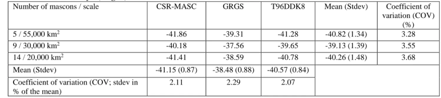
The test with synthetic data shows that the error in recovering the total mass is ~5% regardless of 314
the mascon resolution. On one hand, using different solutions over the same distribution leads to 315
a Coefficient of Variation (COV) of ~3.5% (Table 4). On the other hand, using different 316
distributions with the same solution leads to a COV of ~2.1 %. The similarity between the solutions 317
(Fig. 4D; Table 4) proves a clear improvement in GRACE processing with the latest solutions 318
from the 2016-2018 era such as CSR RL06. When considering an ample TWS anomaly like the 319
GOA, solutions are usually leading to similar observations. However, it might not be the case when 320
considering low amplitude signals which are closer to the noise level, and more sensitive to the 321
processing strategy. 322
These results are compared with results from previous studies performed over the same area in 323
Table 1. Baur (2013), Jacob (2012), and Wahr (2016) found ice loss rates within the range 47-52 324
Gt/yr, which is in good agreement with our results (Fig. 5). Chen et al. (2006), Luthcke et al. (2008) 325
and Tamisiea et al. (2005) found significantly higher ice loss rates. This can be related to the 326
shorter TWS time-series and the larger uncertainties associated with the early releases of GRACE 327
TWS data. Our results are close to the estimates from studies using different methods (Berthier et 328
al., 2010; Gardner et al., 2013; Larsen et al., 2015, values are listed in the introduction). 329
Differences in GRACE Level-3 data interpretation strategy can lead to discrepancies with 330
estimates from other authors. The use of a constrained forward modelling strategy can lead to 331
lower values, as it only recovers the signal spatially correlated to glaciers (see e.g. Long et al. 332
2016, who provide an example for groundwater depletion). The injection of a distribution 333
constraint is known to reduce contributions from unwanted signals with contrasting spatial 334
patterns. These signals cannot be focused onto the constraining distribution (Farinotti et al. 2015; 335
Castellazzi et al. 2018). However, the distribution map is a simplification of the reality as it does 336
not consider the intra-mascon heterogeneity of the ice loss signal. This might lead to uncertainties, 337
depending on the level of unaccounted heterogeneity and its location on the distribution map. 338
339
4.3. Mascon-scale ice mass loss
340
In this section, we discuss the reliability of considering mass losses focused over mascon at 341
different scales. For each inversion, the result corresponds to the best fit to reproduce the true 342
GRACE TWS over the GOA. Total per-mascon masses are presented in Table 5, and the spatial 343
patterns of the mean and standard deviation of glacier mass changes are showed in Fig. 6. As 344
discussed previously, we assume that the degree of similarity between the mass losses retrieved 345
using the three solutions represents a good indicator of accuracy. The maximum value of variation 346
within each mascon correspond to ~13, ~25 and ~40% of the mean mass allocated, for the 5, 9 and 347
14-mascon delineations, respectively. It is observed that this variation tends to increase over the 348
East/West extremes of the study area (Table 6; Fig. 6). This corresponds to differences observed 349
by comparing the low-resolution GRACE TWS trend maps (Fig. 4) which propagates into the 350
inversion results. These variations due to differences in processing strategies increase with the 351
spatial resolution (Table 6); that is the estimates for the 14-mascon delineation have the highest 352
level of uncertainty. 353
We evaluate the accuracy of our mass loss estimates by comparison with those from other studies. 354
This comparison is based on the area with the largest mass losses, which are the Saint Elias 355
Mountains and Glacier Bay, according to Luthcke et al. 2013. This was confirmed by Arendt et al. 356
(2013), who showed that the Saint Elias Mountains, Glacier Bay, and Juneau icefield regions 357
present the largest amount of glacier mass losses. Jin et al. (2017) indicated that the Malaspina and 358
Bering glaciers, belonging to the Saint Elias Mountains, have the largest rates of ice mass losses. 359
10 This is a provisional file, not the final typeset article
Glaciers of the Saint Elias Mountains correspond to mascons 6, 7 and 10 in Luthcke et al. (2008; 360
see Fig. 7A) and mascon 6 in Arendt et al (2013; see Fig. 7B). Our estimates agree with the 361
aforementioned studies which indicate that glaciers of the Saint Elias Mountains have the largest 362
mass loss rates in the region (see Table S2 and Table S3 in the Supplementary Information file). 363
Arendt et al. (2008) used the same delineation and GRACE TWS solution as Luthcke et al. (2008; 364
see Fig. 7A). By down-sampling the solution to the Saint Elias Mountains (cumulating rates from 365
mascons 6, 7 and 10; Fig. 7A in Luthcke et al., 2008), using the ratio of ice area in each mascon 366
over the period 2003-2007, they obtained 20.6 ±3.0 Gt/yr of ice loss for the glaciers of the Saint 367
Elias Mountains. Luthcke et al. (2008) calculated 36 ±2.0 and 30 ±2.0 Gt/yr of ice mass loss by 368
using GRACE data for 2003-2006 and 2003-2007, respectively. First, we compare the results from 369
these two studies with our estimates over the period 2002-2017 (Table 7), and we create a temporal 370
subset from our estimates to make our comparison insensitive to discordances in the time-period 371
considered. 372
Comparing our results with two other studies (Arendt et al., 2008; Lutchke et al., 2008) after 373
applying similar spatial constraints, we observe that the results from Arendt et al. (2008) are similar 374
to our estimates regardless of the mascon delineation considered. Results from Luthcke et al. 375
(2008) are generally larger than our estimates, as do most other studies using GRACE data from 376
the 2003-2006 time-period. However, we note similarities for mascon numbers 5, 6 and 7, at the 377
center of the GOA, where the mass change is the strongest (Table S3). This observation coincides 378
with our visual observation of the spatial patterns of mass losses (Table 6). It points out that the 379
weaker signal at the extreme East-West side is sensitive to the processing strategy and its 380
corresponding residual noise pattern. 381
Considering the ice loss rates over the same time-period allows us to understand the source of the 382
differences observed between our results and these two studies. To do so, we calculated the ratios 383
between the trend at the center of the Saint Elias Mountains derived from the full length of the 384
GRACE time-series, and the trend computed after selecting a temporal subset corresponding to 385
the time scale of their study (Fig. S2). All the trends have been determined by using the method 386
described in Sup. Mat. (Fig. S1). We then reported the ratios obtained over the trend rates from 387
our focused trend maps. The results from our study over these short periods (i.e. 2003-2006 and 388
2003-2007) are ~20% larger than those over the period 2002-2017 (Table 7). We conclude that the 389
use of a shorter time-series plays a significant role in the differences observed with results from 390
other studies, and that these differences may not only be due to the choice of GRACE processing 391
strategy. In other words, estimations built from a short GRACE times-series (3-4 years from 2003) 392
have overestimated the long-term glacial mass loss by ~20%. The inter-annual variability of the 393
snow cover might strongly influence the TWS while considering short time-series. 394
We also compared our results over the Saint Elias Mountain with the mascon solution from NASA 395
GSFC (v2.4; Luthcke et al. 2013; see Fig. S2), which considers GRACE data from 2003 to 2016. 396
The mass loss rate obtained by using this dataset over the Saint Elias Mountains is 24.85 ±2.1 397
Gt/yr. Over the same area, we estimate the glacial mass loss at 22.01 ±0.89, 21.57 ±1.18 and 21.41 398
±1.64 Gt/yr for our three mascon resolutions. Our results are very close to those from the NASA 399
GSFC mascon data (v02.4), and the slight difference might be attributed to the difference in time-400 series length (2003-2016 vs. 2002-2017). 401 402 4.4. Inversion residuals 403
Residual maps are produced by subtracting the FM of the high resolution mass distribution maps 404
from the actual GRACE TWS signal. The amplitude of the residual decreases with the mascon 405
11 This is a provisional file, not the final typeset article
extent. This confirms the ability to retrieve the total mass when a large number of mascons is used. 406
However, as previously discussed, it is at the cost of a lower accuracy at the mascon scale. 407
We note that the inversion residuals from the GRGS and T96DDK8 solutions have similar spatial 408
patterns. It is negligible inland (values below ±2 cm/yr) and more important near the ocean (close 409
to -5 cm/yr). The high absolute residual value near the ocean could be due to coastal glaciers 410
covered by the land mask, implying that a part of the signal from these glaciers is not recovered 411
through the focusing procedure. 412
Following Wahr et al. (2006), and Ramillien et al. (2017), the GRACE TWS data contain noise 413
patterns from measurements and processing errors. We compare the amplitude of the noise with 414
the residuals of the inversion procedure to verify the performance of the inversion (Fig. 8). We 415
consider that the noise level can be approximated by observing the maximum amplitude of mass 416
trends in the Pacific Ocean at similar latitudes than our study area. We found values of ~1.4, 1.6, 417
and 1.5 cm/yr for the CSR-MASC, GRGS, and T96DDK8 solutions, respectively. These values 418
are close to the residuals (values between [-2:+2] cm/yr), which suggests that the remaining signal 419
left after mass concentration might not be attributed to the glacial mass loss. 420
421
Conclusions 422
This study shows a downscaling approach of GRACE TWS data can be used to retrieve a high 423
resolution ice mass loss. We tested three GRACE solutions and three uniform focusing 424
delineations, and applied an inversion method which relies on fitting iteratively a spatially 425
constrained FM. We used the three solutions at the same truncation level (i.e. resolution) in order 426
to isolate the effect of the processing strategy applied to the GRACE data from Levels 1 to 3. From 427
our study, we can draw three key findings. 428
First, synthetic simulations indicate that the forward modelling approach is efficient, with mean 429
error of ~2.5% when considering the total mass loss over the Gulf Of Alaska (GOA), and below 430
10% when considering masses at the mascon-scale and with mascons up to 30,000 km2. It also 431
shows that our inversion procedure is relatively insensitive to non-ice masses such as soil moisture. 432
Second, at the scale of the GOA, the resolution of the mass concentration units (referred to as 433
mascon) and the choice of the GRACE solution strategy only account for an uncertainty of ~2-4% 434
in the total mass estimation. The three solutions provide approximatively the same total mass loss 435
(~40 Gt/yr) over the era 2002-2017. 436
Third, at the scale of a mascon of 30,000 km2 or larger, the focusing procedure recovers well the 437
regional mass loss signal. At this scale, the mascon over the GOA contain from 1 to 9 Gt/yr of ice 438
mass loss, the highest mass loss rates being at the centre of the area, in the Saint Elias Mountains. 439
Variations between solutions reach 40% of the mean signal when considering high resolution 440
mascons of 20,000 km2. Residuals are of the same order of magnitude as the noise level of GRACE 441
TWS solutions. Thus, the glacier signals are well retrieved when using an inversion with a uniform 442
constrained FM, and the distribution map is efficient at concentrating the mass loss observed by 443
GRACE. 444
We compared our results with estimates reported in the literature and found a good agreement with 445
studies using GRACE solutions from recent releases and time-series of more than 8 years. The 446
first studies using GRACE data published during the 2005-2008 era generally overestimated the 447
long-term ice mass loss at the GOA scale due to the data time-span, the interpretation strategy, and 448
possibly the use of early release of GRACE data. Comparing our ice loss map at the highest 449
resolution with those of Arendt et al. (2008) and the mascon solution from NASA GSFC over the 450
Saint Elias Mountains, we obtained relatively similar ice loss rates. This area of comparison is at 451
12 This is a provisional file, not the final typeset article
the center of the GOA, where our results are the most reliable, with mass losses and Signal-Noise 452
Ratio at the highest. 453
To our knowledge, this is the first study presenting a focused and spatially constrained ice loss 454
map over the GOA. Comparison of our findings with results from other data sources (i.e., 455
altimetry) could help further assessing the accuracy of our estimates. Constraining the focusing 456
procedure using a heterogeneous mass loss map from other data sources would allow to cope with 457
the heterogeneity of the losses, which is partially unaccounted for in this study. The findings of 458
this study could help integrating an ice mass loss module into large-scale hydrological models; 459
providing a framework to better understand the effect of climate change on the hydrological cycle 460
of the main river basins of the GOA area. 461
462
Acknowledgments
463
The authors would like to thank Wei Feng (Chinese Academy of Sciences) for the development of 464
GRAMAT (GRACE Matlab Toolbox) which was used to process GRACE data. The authors wish 465
to gratefully acknowledge the financial support of the Natural Sciences and Engineering Research 466
Council of Canada (NSERC) and the Yukon Energy Corporation (YEC). 467
468
Author Contributions Statement
469
Cheick Doumbia performed the data analysis and wrote the manuscript. Pascal Castellazzi trained 470
the first author to process GRACE data, verified the results, and contributed to the writing of the 471
manuscript. Alain N. Rousseau designed and led the project, supervised the first author, and 472
contributed to the writing of the manuscript. Macarena Amaya helped to build a comprehensive 473
literature review on the topic. 474
475
Conflict of Interest Statement
476
The authors declare that no personal, professional or financial relationships can be construed as a 477
conflict of interest. 478
479
Contribution to the Field Statement
480
This paper presents how low-resolution time-variable gravity data can be downscaled to better 481
understand ice mass loss at the regional scale. In the Gulf of Alaska, a large-scale signal of mass 482
loss, extending over a ~1500-km-long stretch, is observed by the two satellites of a well-known 483
gravity recovery mission (GRACE). This anomaly corresponds to ice mass loss from numerous 484
glaciers located along the southern coast of Alaska (USA) and Yukon (Canada). While the total 485
mass can be recovered using GRACE data, the resolution of such observation is too low to derive 486
ice mass loss at the scale of glaciers, ice fields, or at the regional scale. We present how, using a 487
distribution map of the glaciers, GRACE signal can be focused to smaller spatial units. More 488
importantly, we explore the limits of the procedure: while the processing strategy chosen to process 489
GRACE data is not important when interpreting the signal at the scale of the anomaly, it becomes 490
an important parameter while trying to discriminate small-scale contributors. 491
492
13 This is a provisional file, not the final typeset article
References
493
Arendt A, Luthcke S, Gardner A, O’Neel S, Hill D, Moholdt G, Abdalati W (2013) Analysis of a 494
GRACE global mascon solution for Gulf of Alaska glaciers. Journal of Glaciology 495
59:913–924 . doi: 10.3189/2013JoG12J197 496
Arendt AA, Luthcke SB, Hock R (2009) Glacier changes in Alaska: can mass-balance models 497
explain GRACE mascon trends? Annals of Glaciology 50:148–154 . doi: 498
10.3189/172756409787769753 499
Arendt AA, Luthcke SB, Larsen CF, Abdalati W, Krabill WB, Beedle MJ (2008) Validation of 500
high-resolution GRACE mascon estimates of glacier mass changes in the St Elias 501
Mountains, Alaska, USA, using aircraft laser altimetry. Journal of Glaciology 54:778– 502
787 . doi: 10.3189/002214308787780067 503
Baraer M, Mark BG, Mckenzie M, Condom T, Bury J, Huh K-I, Portocarrero C, Gómez J, 504
Rathay S (2012) Glacier recession and water resources in Peru’s Cordillera Blanca. J 505
Glaciol 58:134–150 . doi: 10.3189/2012JoG11J186 506
Baur O, Kuhn M, Featherstone WE (2013) Continental mass change from GRACE over 2002– 507
2011 and its impact on sea level. Journal of Geodesy 87:117–125 . doi: 10.1007/s00190-508
012-0583-2 509
Beamer JP, Hill DF, Arendt A, Liston GE (2016) High-resolution modeling of coastal freshwater 510
discharge and glacier mass balance in the Gulf of Alaska watershed: COASTAL FWD 511
AND GVL IN GOA WATERSHED. Water Resources Research 52:3888–3909 . doi: 512
10.1002/2015WR018457 513
Berthier E, Schiefer E, Clarke GKC, Menounos B, Rémy F (2010) Contribution of Alaskan 514
glaciers to sea-level rise derived from satellite imagery. Nature Geoscience 92-95. doi: 515
10.1038/ngeo737 516
Blanchon D, Boissière A (2009) Atlas mondial de l’eau: de l’eau pour tous 517
Castellazzi P, Burgess D, Rivera A, Huang J, Longuevergne L, Demuth MN ( 2019) Glacial melt 518
and potential impacts on water resources in the Canadian Rocky Mountains. Water 519
Resources Research, 55. doi: 10.1029/2018WR024295 520
Castellazzi P, Longuevergne L, Martel R, Rivera A, Brouard C, Chaussard E (2018) Quantitative 521
mapping of groundwater depletion at the water management scale using a combined 522
GRACE/InSAR approach. Remote Sensing of Environment 205:408–418 . doi: 523
10.1016/j.rse.2017.11.025 524
Castellazzi P, Martel R, Rivera A, Huang J, Pavlic G, Calderhead AI, Chaussard E, Garfias J, 525
Salas J ( 2016) Groundwater depletion in Central Mexico: Use of GRACE and InSAR to 526
support water resources management, Water Resources Research, 52, 5985– 6003, 527
doi:10.1002/2015WR018211. 528
Chen J, Ohmura A (1990) Estimation of Alpine glacier water resources and their change since 529
the 1870s. IAHS (Symopsium at Lausanne, 1990 – Hydrology in Mountainous Regions 530
I):127–135 531
Chen JL, Tapley BD, Wilson CR (2006) Alaskan mountain glacial melting observed by satellite 532
gravimetry. Earth and Planetary Science Letters 248:368–378 . doi: 533
10.1016/j.epsl.2006.05.039 534
Chen JL, Wilson CR, Blankenship D, Tapley BD (2009) Accelerated Antarctic ice loss from 535
satellite gravity measurements. Nature Geoscience 2:859–862 . doi: 10.1038/ngeo694 536
14 This is a provisional file, not the final typeset article
Chen JL, Wilson CR, Li J, Zhang Z (2015) Reducing leakage error in GRACE-observed long-537
term ice mass change: a case study in West Antarctica. Journal of Geodesy 89:925–940 . 538
doi: 10.1007/s00190-015-0824-2 539
Farinotti D, Longuevergne L, Moholdt G, Duethmann D, Mölg T, Bolch T, Vorogushyn S, 540
Güntner A (2015) Substantial glacier mass loss in the Tien Shan over the past 50 years. 541
Nature Geoscience 8:716–722 . doi: 10.1038/ngeo2513 542
Frans C, Istanbulluoglu E, Lettenmaier DP, Fountain AG, Riedel J (2018) Glacier Recession and 543
the Response of Summer Streamflow in the Pacific Northwest United States, 1960-2099. 544
Water Resources Research 54:6202–6225 . doi: 10.1029/2017WR021764 545
Gardner AS, Moholdt G, Cogley JG, Wouters B, Arendt AA, Wahr J, Berthier E, Hock R, 546
Pfeffer WT, Kaser G, Ligtenberg SR, Bolch T, Sharp MJ, Hagen JO, van den Broeke M, 547
Paul F (2013) A Reconciled Estimate of Glacier Contributions to Sea Level Rise: 2003 to 548
2009. Science 340:6134-852 . doi: 10.1126/science.1234532 549
Geruo A, Wahr J, Zhong S (2013) Computations of the viscoelastic response of a 3-D 550
compressible Earth to surface loading: an application to Glacial Isostatic Adjustment in 551
Antarctica and Canada. Geophysical Journal International 192:557–572 . doi: 552
10.1093/gji/ggs030 553
GLIMS, NSIDC (2005, updated 2018) Global Land Ice Measurements from Space glacier 554
database. Compiled and made available by the international GLIMS community and the 555
National Snow and Ice Data Center, Boulder CO, USA. doi: 10.7265/N5V98602 556
Hingray B, Picouet C, Musy A (2014) Hydrologie 2 Une science pour l’ingénieur, 1ère édition. 557
PPUR 558
Hock, R. (1999), A distributed temperature index ice and snow melt model including potential 559
direct solar radiation, Journal of Glaciology, 45(149), 101-111, doi: 560
10.3189/S0022143000003087 561
Hooke R, Jeeves TA (1961) `` Direct Search’’ Solution of Numerical and Statistical Problems. 562
Journal of the ACM 8:212–229 . doi: 10.1145/321062.321069 563
Huss M, Hock R (2018) Global-scale hydrological response to future glacier mass loss. Nature 564
Climate Change 8:135–140 . doi: 10.1038/s41558-017-0049-x 565
Jacob T, Wahr J, Pfeffer WT, Swenson S (2012) Recent contributions of glaciers and ice caps to 566
sea level rise. Nature 482:514–518 . doi: 10.1038/nature10847 567
Jin S, Feng G (2016) Uncertainty of grace-estimated land water and glaciers contributions to sea 568
level change during 2003–2012. 6189–6192 . doi: 10.1109/IGARSS.2016.7730617 569
Jin S, Zhang TY, Zou F (2017) Glacial density and GIA in Alaska estimated from ICESat, GPS 570
and GRACE measurements: Glacial Density and GIA in Alaska. Journal of Geophysical 571
Research: Earth Surface 122:76–90 . doi: 10.1002/2016JF003926 572
Jin S, Zou F (2015) Re-estimation of glacier mass loss in Greenland from GRACE with 573
correction of land–ocean leakage effects. Global and Planetary Change 135:170–178 . 574
doi: 10.1016/j.gloplacha.2015.11.002 575
Kienholz C, Herreid S, Rich JL, Arendt AA, Hock R, Burgess EW (2015) Derivation and 576
analysis of a complete modern-date glacier inventory for Alaska and northwest Canada. 577
Journal of Glaciology 61:403–420 . doi: 10.3189/2015JoG14J230 578
Kolda TG, Lewis RM, Torczon V (2003) Optimization by Direct Search: New Perspectives on 579
Some Classical and Modern Methods. SIAM Review 45:385–482 . doi: 580
10.1137/S003614450242889 581
15 This is a provisional file, not the final typeset article
Kusche J (2007) Approximate decorrelation and non-isotropic smoothing of time-variable 582
GRACE-type gravity field models. Journal of Geodesy 81:733–749 . doi: 583
10.1007/s00190-007-0143-3 584
Kusche J, Schmidt R, Petrovic S, Rietbroek R (2009) Decorrelated GRACE time-variable 585
gravity solutions by GFZ, and their validation using a hydrological model. Journal of 586
Geodesy 83:903–913 . doi: 10.1007/s00190-009-0308-3 587
Larsen CF, Motyka RJ, Arendt AA, Echelmeyer KA, Geissler PE (2007) Glacier changes in 588
southeast Alaska and northwest British Columbia and contribution to sea level rise. 589
Journal of Geophysical Research 112: . doi: 10.1029/2006JF000586 590
Larsen, C. F., E. Burgess, A. A. Arendt,S. O’Neel, A. J. Johnson, and C. Kienholz (2015), 591
Surface melt dominates Alaskaglacier mass balance,Geophys. Res. Lett.,42, 5902–5908, 592
doi:10.1002/2015GL064349 593
Long D, Chen X, Scanlon BR, Wada Y, Hong Y, Singh VP, Chen Y, Wang C, Han Z, Yang W 594
(2016) Have GRACE satellites overestimated groundwater depletion in the Northwest 595
India Aquifer? Scientific Reports 6: . doi: 10.1038/srep24398 596
Longuevergne L, Scanlon BR, Wilson CR (2010) GRACE Hydrological estimates for small 597
basins: Evaluating processing approaches on the High Plains Aquifer, USA: GRACE 598
HYDROLOGICAL ESTIMATES FOR SMALL B. Water Resources Research 46: . doi: 599
10.1029/2009WR008564 600
Luthcke SB, Arendt AA, Rowlands DD, McCarthy JJ, Larsen CF (2008) Recent glacier mass 601
changes in the Gulf of Alaska region from GRACE mascon solutions. Journal of 602
Glaciology 54:767–777 . doi: 10.3189/002214308787779933 603
Luthcke SB, Sabaka TJ, Loomis BD, Arendt AA, McCarthy JJ, Camp J (2013) Antarctica, 604
Greenland and Gulf of Alaska land-ice evolution from an iterated GRACE global mascon 605
solution. Journal of Glaciology 59:613–631 . doi: 10.3189/2013JoG12J147 606
MATLAB and Statistics Toolbox Release 2017a, The MathWorks, Inc., Natick, Massachusetts, 607
United States. 608
Peltier, W.R., Argus, D.F. and Drummond, R. (2015) Space geodesy constrains ice-ag terminal 609
deglaciation: The global ICE-6G_C (VM5a) model. J. Geophys. Res. Solid Earth, 120, 610
450-487, doi:10.1002/2014JB011176 611
Pfeffer WT, Arendt AA, Bliss A, Bolch T, Cogley JG, Gardner AS, Hagen J-O, Hock R, Kaser 612
G, Kienholz C, Miles ES, Moholdt G, Mölg N, Paul F, Radić V, Rastner P, Raup BH, 613
Rich J, Sharp MJ, The Randolph Consortium (2014) The Randolph Glacier Inventory: a 614
globally complete inventory of glaciers. Journal of Glaciology 60:537–552 . doi: 615
10.3189/2014JoG13J176 616
Pomeroy JW, Gray DM, Brown T, Hedstrom NR, Quinton WR, Granger RJ, Carey SK (2007), 617
The cold regions hydrological model: a platform for basing process representation and 618
model structure on physical evidence, Hydrological Processes, 21(19), 2650-2667, doi: 619
10.1002/hyp.6787 620
Radić V, Hock R (2011) Regionally differentiated contribution of mountain glaciers and ice caps 621
to future sea-level rise. Nature Geoscience 4:91–94 . doi: 10.1038/ngeo1052 622
Ramillien G, Frappart F, Seoane L (2017) La mission de gravimétrie spatiale GRACE: 623
instruments et principe de fonctionnement, in N Baghdadi and M Zribi (Eds.), 624
Observations des surfaces continentales par télédétection micro-onde: techniques et 625
méthodes (pp. 281-297), ISTE Editions Ltd. 27-37 St Georges’s Road London SW19 626
4EU UK 627
16 This is a provisional file, not the final typeset article
Raup B, Racoviteanu A, Khalsa SJS, Helm C, Armstrong R, Arnaud Y (2007) The GLIMS 628
geospatial glacier database: A new tool for studying glacier change. Global and Planetary 629
Change 56:101–110 . doi: 10.1016/j.gloplacha.2006.07.018 630
Rodell M, Houser PR, Jambor U, Gottschalck J, Mitchell K, Meng C-J, Arsenault K, Cosgrove 631
B, Radakovich J, Bosilovich M, Entin JK, Walker JP, Lohmann D, Toll D (2004) The 632
Global Land Data Assimilation System. Bulletin of the American Meteorological Society 633
85:381–394 . doi: 10.1175/BAMS-85-3-381 634
Save H, Bettadpur S, Tapley BD (2016) High-resolution CSR GRACE RL05 mascons: HIGH-635
RESOLUTION CSR GRACE RL05 MASCONS. Journal of Geophysical Research: Solid 636
Earth 121:7547–7569 . doi: 10.1002/2016JB013007 637
Swenson S, Wahr J, Milly PCD (2003) Estimated accuracies of regional water storage variations 638
inferred from the Gravity Recovery and Climate Experiment (GRACE). Water Resources 639
Research 39:1223 . doi: 10.1029/2002WR001808 640
Tamisiea ME, Leuliette EW, Davis JL, Mitrovica JX (2005) Constraining hydrological and 641
cryospheric mass flux in southeastern Alaska using space-based gravity measurements. 642
Geophysical Research Letters 32: . doi: 10.1029/2005GL023961 643
Tapley BD, Bettadpur S, Watkins M, Reigber C (2004) The gravity recovery and climate 644
experiment: Mission overview and early results: GRACE MISSION OVERVIEW AND 645
EARLY RESULTS. Geophysical Research Letters 31:n/a-n/a . doi: 646
10.1029/2004GL019920 647
Wahr J, Burgess E, Swenson S (2016) Using GRACE and climate model simulations to predict 648
mass loss of Alaskan glaciers through 2100. Journal of Glaciology 62:623–639 . doi: 649
10.1017/jog.2016.49 650
Wahr J, Molenaar M, Bryan F (1998) Time variability of the Earth’s gravity field: Hydrological 651
and oceanic effects and their possible detection using GRACE. Journal of Geophysical 652
Research: Solid Earth 103:30205–30229 . doi: 10.1029/98JB02844 653
Wahr J, Swenson S, Velicogna I (2006) Accuracy of GRACE mass estimates. Geophysical 654
Research Letters 33:L06401 . doi: 10.1029/2005GL025305 655
Yirdaw SZ, Snelgrove KR, Seglenieks FR, Agboma CO, Soulis ED (2009) Assessment of the 656
WATCLASS hydrological model result of the Mackenzie River basin using the GRACE 657
satellite total water storage measurement. Hydrological Processes 23:3391–3400 . doi: 658 10.1002/hyp.7450 659 660 661
In review
17 This is a provisional file, not the final typeset article
Figure 1: Glaciers of the GOA and footprints of the study area considered in studies using 662
GRACE data to assess glacier melt. The study area considered here is identified as Zone 10. 663
664
Figure 2: Glacier distribution map used to focus GRACE trend maps. Three arbitrary mascon 665
delineations are presented: (A) 5 mascons with an average area of ~55,000 km2, (B) 9 mascons 666
with an average area of ~30,000 km2, and (C) 14 mascons with an average area of ~20,000 km2. 667
668
Figure 3: (A) Synthetic mass randomly allocated to pixels corresponding to glaciers. (B) Soil 669
Moisture trend from GLDAS Noah Land Surface Model (LSM) v2.1. (C) Forward Model (FM) of 670
A overlaid on B, representing a realistic reproduction of the GRACE trend signal derived from 671
known masses. It includes both concentrated and diffuse mass changes in realistic proportions. 672
(D) Example of a high resolution glacier mass loss map retrieved by applying the inversion 673
procedure over (C) and using the 5-mascon delineation shown in Fig. 2A. This synthetic test allows 674
to assess the inversion procedure and its ability to retrieve glacier mass losses at high resolution. 675
Results are presented in Table S1 (see Supplementary Information). 676
677
Figure 4: TWS signal trend over the study area using the three GRACE solutions: (A) CSR-678
MASC, (B) GRGS, (C) T96DDK8, and (D) near-monthly time-series of TWS change in WTE for 679
the period 2012-2017 observed at the center of the anomaly. 680
681
Figure 5: Comparison between glacier mass loss estimates from this study with those of other 682
studies. Zones refer to the glacier coverage considered in the published literature, as listed in 683
Table 1. 684
685
Figure 6: High resolution mapping according to the three mass distribution scenarios (Fig. 2): 686
mean mass loss (A,B,C) and standard deviation (D,E,F). Maps are presented in order of focusing 687
resolution: (A-D) 5-, (B-E) 9-, and (C-F) 14-mascon delineations. Two different scales of the same 688
color maps are used for (A-C) and (D-F). 689
690
Figure 7: Overlay of mascon delineations from other studies over the glacier distribution map 691
used in this study: (A) delineation used by Luthcke et al. (2008); (B) delineation used by Arendt et 692
al. (2013), in which Glacier Bay is included in mascon 6, corresponding to the Saint Elias 693
Mountains (Table S2 in the Supplementary Information file). 694
695
Figure 8: Residual maps of the focusing procedure in WTE. These maps represent the signal 696
remaining after subtracting the best forward model (FM) to the actual GRACE TWS signal. 697 698 699 700 701 702 703 704 705 706 707
In review
18 This is a provisional file, not the final typeset article
Table 1: Estimates of glacier mass loss in the GOA according to different authors. 708
Study areas (Fig. 1)
Authors (Year) Data time
period
Estimated mass loss (Gt/yr)
Data source Glaciers area considered (km2)
0 Tamisiea et al. 2005 2002–2004 -110 GRACE 87,000
1 Chen et al. 2006 2002–2005 -101 GRACE ~90,957
2 Luthcke et al. 2008 2003–2006 -102 GRACE ~82,505
2003–2007 -84
3 Arendt et al. 2008 2003–2007 -20.6 GRACE 32,900
4 Jacob et al. 2012 2003–2010 -46 GRACE ~90,000
5 Arendt et al. 2013 2003–2009 -61 GRACE 82,505
2003–2010 -65
2004–2010 -71
6 Baur et al. 2013 (2002-2011)a -56 GRACE with
geocenter correction ~80,000 (2002-2011)b -47 GRACE without geocenter correction
7 Beamer et al. 2016 2004-2013 -60,1 GRACE 72,302
8 Wahr et al. 2016 2002-2014 -52 GRACE and
Meteorological model
~72,600
9 Jin et al. 2017 2003-2009 -57.5 ICESat altimetry
and GRACE
86,715 709
Table 2: Description of the three mascon delineations. 710
Mascon number Total Surface (km²) Average (km²) Standard deviation (km²)
5 272,400 54,480 1,214
9 282,970 31,441 1,657
14 278,760 19,911 690
711
Table 3: Errors in recovering known synthetic masses allocated over the distribution map (Fig. 712
3). Each test is performed with and without taking into account a diffuse mass representing e.g. 713
soil moisture changes. 714 Total mass recovery error (without diffuse mass) - % Total mass recovery error (with diffuse mass) - %
Mean error per mascon (without
diffuse mass) - %
Mean error per mascon (with diffuse mass) - % Maximum error per mascon (without diffuse mass) - % Maximum error per mascon (with diffuse mass) - % 5 Mascons 55,000 km2-scale 2.514 5.071 2.435 5.141 8.406 9.937 Mascons 30,000 km2-scale 2.683 5.207 9.544 10.347 15.508 17.472 14 Mascons 20,000 km2-scale 3.244 4.761 13.568 14.600 55.994 68.195 715 716 717 718 719 720