HAL Id: hal-01824238
https://hal.archives-ouvertes.fr/hal-01824238
Preprint submitted on 27 Jun 2018
HAL is a multi-disciplinary open access
archive for the deposit and dissemination of sci-entific research documents, whether they are pub-lished or not. The documents may come from teaching and research institutions in France or abroad, or from public or private research centers.
L’archive ouverte pluridisciplinaire HAL, est destinée au dépôt et à la diffusion de documents scientifiques de niveau recherche, publiés ou non, émanant des établissements d’enseignement et de recherche français ou étrangers, des laboratoires publics ou privés.
Fisheries management: what uncertainties matter?
Jules Selles
To cite this version:
Fisheries management: what uncertainties matter?
1
Selles Jules1, 2*
2
1IFREMER (Institut Français de Recherche pour l’Exploitation de la MER), UMR MARBEC, Avenue Jean 9 3
Monnet, BP171, 34203 Sète Cedex France. 4
2LEMNA, Université de Nantes, IEMN-IAE, Chemin de la Censive-du-Tertre, BP 52231, ´44322 Nantes 5
Cedex France. 6
*corresponding author, email: [email protected], tel: +33 (0)779490657 7
8
Abstract — 9
Uncertainty is pervasive in fisheries management. Bioeconimists have undertaken
long-10
standing effort to derive economically optimal management rules under uncertainty and
11
provide explicitly optimal feedback solutions. Based on this body of work, we determine the
12
importance of different kinds of uncertainty in the definition of harvest control rules. The
13
performances of harvest policies which dictate how harvest is determined as a function of
14
the state of the resource are sensitive to uncertainty. We discuss six sources of uncertainties
15
and illustrate how these have affected the management process. We then describe how
16
those classes of uncertainty affect optimal harvest control rules. We summarize the
17
conclusions of economists based on structural assumptions affecting objective functions
18
under different classes of uncertainties. We identify common classes of harvest control rules
19
and the resulting precaution of the harvest strategy. Finally, we discuss the opportunities to
20
develop fully adaptive management to decide upon structural assumptions through the
21
extension of Markov decision process and feedback solutions to complex models.
22 23
Keywords— Bioeconomic modeling; Uncertainty; Fisheries management; Optimal resource 24
management; Harvest policy; Harvest strategies; Control rules.
25 26
1 Introduction
27
Despite many fisheries are highly regulated, overexploitation of fish stocks is still a 28
problem worldwide and rebuilding fisheries is central in scientists debates (Ricard et al. 29
2009, Worm et al. 2009, Costello et al. 2016, Froese et al. 2018). The failures of fishery 30
management have been linked to the inherent characteristics of fish stocks and the 31
influence of the global market-driven by growing demand for fishery products (Seijo et 32
al. 1998, Cochrane 2000, Caddy & Seijo 2005, Sethi et al., 2010, Collette et al. 2011, 33
Longo & Clark 2012, Pons et al. 2017). Management difficulties have been also attributed 34
to ignoring uncertainties that characterize fishery systems and to respond with a lack of 35
caution in management. Risks1 associated with uncertainties and multiple objectives
36
permeate fisheries management (Francis & Shotton 1997, Cochrane 2000, Hilborn 2007, 37
Sethi 2010). Many fisheries have experienced overfishing2 as a result of risky and short
38
sighted management policies (Clark 1973b, Garcia 1996, Hilborn et al. 2001, Grafton 39
2007, Clark 2010). 40
In face of uncertainty, the concept of the precautionary approach has been employed 41
widely among nations and fishery agencies (e.g. in Regional Fishery Management 42
Organisations, RFMOs, de Bruyn et al. 2013) to account explicitly for uncertainties in 43
decision making (FAO 1996, Garcia 1996). Precautionary principles are the basis to 44
ensure that the lack of full scientific knowledge (i.e. certainty) should not be an incentive 45
to postpone effective measure to prevent unsustainable exploitation (UNCED, 1993). 46
Besides, they have been translated into the adoption of management reference points to 47
avoid risks. Limit and target reference points have been adopted and management 48
decision should ensure that the risk of exceeding limit reference points is very low and 49
that target reference points should be respected on average (FAO 1996). The biomass 50
(BMSY) that can produce the maximum sustainable yield (MSY) constitutes the central
51
reference point for fisheries referred to in international agreements and instruments 52
(UNCLOS 1982, UNFSA 1995, FAO 1995). Alongside the implementation of 53
precautionary principles, the Ecosystem-Based Fisheries Management (EBFM, FAO 54
2003, Garcia et al. 2003, Pikitch et al. 2004) has promoted the development of complex 55
1 Risk entails the ideas of uncertainty and loss, the Food and Agriculture Organisation (FAO) refers to
average forecasted loss (FAO, 1996).
2 Biological and economic overfishing (Murawski 2000 defines overfishing in the context of
models integrating all features of the social-ecological system encompassing the fishery. 56
Such Integrated Ecological–Economic Fisheries Models (IEEFMs or simply bioeconomic 57
models) have been increasingly used in the support of fisheries management with the 58
aim to account for complex feedbacks effect betweenfishing activities, and ecosystem 59
dynamics (for a review see Lehuta et al. 2016 and Nielsen et al. 2018). However, the 60
increasing complexities of IEEFMs reduce confidence in forecasting and the ability to 61
disentangle the way in which uncertainty is propagated (Garcia & Charles 2007, Schrank 62
& Pontecorvo 2007, Rochet and Rice 2009, Kraak et al. 2010, Planque 2015). In face of 63
such difficulties, Harvest Control Rules (HCRs) have been promoted to enhance 64
transparency and to consider explicitly the ecological, economic and social goals of the 65
triple bottom line (Cochrane 2000, Hilborn 2007). HCRs provide a simple scientific 66
based management strategy which depends on available data, knowledge and 67
management objectives (Punt 2010). The main contribution of the implementation of 68
HCRs is the integration of the scientific advice into the political realm through the direct 69
proposition of management strategy to deciders (Kvamsdal, 2016). However, the 70
construction of HCRs is mainly based on empirical work and may fail to take into 71
account key uncertainties of the fishery system (Deroba & Bence 2008, Liu et al. 2016). 72
The bioeconomics literature on renewable resource and fishery management models 73
several classes of uncertainty and provide explicitly optimal feedback solutions. The 74
framework considers a social planner seeking to maximize the net present value of the 75
fishery. Optimal Instead of relying only on simulation methods to evaluate the 76
performance of control rules, HCRs derived from such bioeconomic models can provide 77
guidelines on how setting harvest policies when uncertainty is considered. 78
The objective of this review is to bring insights into the importance of different kinds of 79
uncertainty in the definition of harvest control rules. The pursuit of this goal raises an 80
important question: what uncertainties matter when determining control rules? We 81
base our review on the long-standing effort to derive economically optimal management 82
rules under uncertainty. First, we describe the place of bioeconomic modeling approach 83
and feedback solutions in fishery management under different sources of uncertainties 84
arising throughout the management process. Then, we identify the shape and the 85
cautious of optimal management strategies under the source of uncertainties previously 86
identified. Finally, we offer conclusions about the relative importance of different kind of 87
uncertainties on the definition of HCRs. 88
2 Fishery management and uncertainties
89
2.1 Adaptive management, HCRs and MSE
90Modern fishery management promotes adaptive management (Walters, 1986) as the 91
new standard framework to address decision problems under uncertainty. Adaptive 92
management is an approach for simultaneously managing and learning about the 93
resource which consists imply to learn by doing and upgrade management policies with 94
new observations (Williams & Brown 2016). Searching for optimal harvest policy 95
corresponds to an attempt to apply adaptive management to fishery management. Clark 96
and Munro (1975) seminal work was the first attempt to develop feedback solution to 97
fishery management. They defined the optimal harvest rate as a function of the resource 98
level. Bioeconomic feedback solutions have inspired the development HCRs (Kvamsdal 99
et al. 2016). HCRs have been developed in response to the need for less complex 100
decision framework integrating the precautionary approach (Kvamsdal et al. 2016). 101
HCRs consist in a predefined series of actions (i.e. total allowable catch limits, TACs) 102
determined as a response of the observation of the state of the fishery (i.e. biological 103
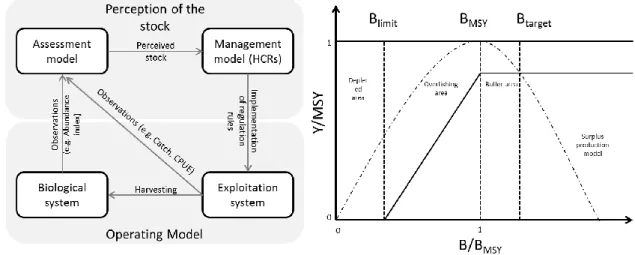
information such as biomass level, Figure 1). However, HCRs are usually not derived 104
from formal IEEFMs optimization models, but are commonly simple rules based on 105
expert opinion. The latter point implies that although HCRs may include several 106
precautionary elements it does not constitute a standalone method to fully account for 107
uncertainties. 108
Management Strategy Evaluation (MSE) has been proposed as leading method for 109
coupling both IEEFMs and HCRs. It consists of associating single species management 110
model (i.e. Virtual Population Analysis VPA): a decision model (HCR) and an ‘’operating 111
model’’ (IEEFM) accounting for alternative modeling hypothesis. MSEs are used to 112
evaluate the extent to which HCR achieve their goals (i.e. reaching Btarget). Given the
113
uncertainty integrated into the operating model, MSEs are used to quantify the risk 114
represented by uncertainties throughout the decision process from observations and 115
assessment models to implementation (Butterworth 2007, Punt et al. 2010). Therefore 116
MSE based on simulation modeling has increasingly been used to evaluate the impact of 117
the main recognized sources of uncertainty in fishery systems (e.g. in the Commission 118
for the Conservation of Southern Bluefin Tuna, Kurota et al. 2010, for a review see Punt 119
et al. 2016). The objective is to find HCRs that are robust to uncertainties and to provide 120
managers with a set of management options that encompass the precautionary 121
approach. 122
123
Figure 1:Conceptual framework of Management strategy evaluation (MSE) (adapted from Kell et al. 2007) 124
and an example of a precautionary constant catch harvest control rule incorporating biomass target 125
(Btarget>BMSY), buffer area and limit (adapted from Froese et al. 2010) with a hypothetical equilibrium yield 126
(Y) from a surplus production model. 127
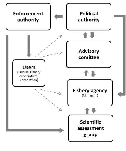
HCRs and MSEs found their essence in ‘top-down’ management scheme where a central 128
regulatory body is in charge of the management and the evaluation of the resource. A 129
typical decision-making structure (Figure 2) is composed of a scientific assessment 130
group giving management advice to managers and to an advisory committee (including 131
resource users) which in turn inform a political authority where responsibility for the 132
final decisions lies. Each country or RFMO has its own institutional chain from scientific 133
fisheries research to political and enforcement decisions (e.g. the Common Fisheries 134
Policy in the European Union, Daw & Gray 2005 or in RFMOs, Lodge et al. 2007). In any 135
case, the central institution typically sets the total allowable catch (TAC) and further 136
inputs restrictions (e.g. seasonal, size catch limit) and specifying the enforcement 137
procedures. 138
Large uncertainties related to resource, economic and social states are common in 139
fishery management and lead to high transaction costs3. Williamson (1985) argued that
140
institutions are established to minimise transaction costs. Thus, in such complex 141
3 Management transaction costs within fisheries can be classified into three categories included in the
fishery management cycle (Abdullah et al. 1998, Figure 3): information costs related to the resource assessment, decision-making costs related to the policy making and operational costs included monitoring, control and enforcement costs (or implementation costs).
systems, the hierarchical and centralized structures of fishery institution have emerged 142
from the high uncertainties in the information on fishery systems (Abdullah 1998, 143
Nielsen 2003). However, the conjunction of centralised institution, high uncertainties 144
levels and complexities in model used for management have narrowed confidence and 145
legitimacy of fishery management institutions (Daw and Gray, 2005, Hauge et al. 2007, 146
Kraak et al. 2010, Dankel et al. 2012). The loss of legitimacy is, in turn, increasing 147
substantially transaction costs related to monitoring and enforcement of regulated 148
fishing activities (Abdullah 1998, Nielsen 2003). Thus, reducing uncertainty 149
surrounding scientific advice should concomitantly decrease management costs. HCRs 150
can facilitate a fisheries governance system where regulators and fishers work together 151
to decide on overall harvest strategy based on predefined HCRs (Kvamsdal et al. 2016). 152
HCRs by integrating management rules (i.e. TAC) in the realm of scientific advice reduce 153
uncertainty with regard to handling and communication of uncertainty (Rosenberg 154
2007, Kraak et al. 2010, Dankel et al. 2012). 155
Nevertheless, HCRs leave aside key political issues such as the allocation of fishing rights 156
imposing high transaction costs. They are mainly distributed on the basis of historical 157
catches negotiation (in RFMOs, Cox 2009, Bailey et al. 2013) rather than economic 158
rationality (Marszalec 2017). Rights-based management such as Individual Transferable 159
Quotas (ITQs), or cooperatives (i.e. Producers Organisations) and community quotas 160
(with or without ITQs) is a complementary solution to provide fishers with good 161
incentives for compliance and efficient allocation regulated through market (Hilborn 162
2004, Grafton et al. 2006, Beddington et al. 2007, Grafton 2008). ITQs, co-management 163
and collective actions have been brought at the forefront as the solution for improving 164
fisheries management (Beddington et al. 2007, Costello et al. 2008, Berkes 2009, 165
Gutiérrez et al. 2011, Deacon 2012). However, theoretical works and empirical 166
evidences have demonstrated that right based management does not constitute a 167
panacea (Clark, 2010, Thebaud et al. 2012, Melnychuk et al. 2012). Co-management by 168
delegating a part of management tasks to user-organizations can substantially reduce 169
transactions by decreasing monitoring and control of activity (Van Hoof, 2009). 170
Furthermore, co-management can increase the legitimacy of regulations and social 171
norms (Jentoft 1998, Nielsen 2003). 172
173
Figure 2: Conceptual decision-making structure in fisheries management (adapted from Cochrane 2000). 174
2.2 Uncertainty in fishery management
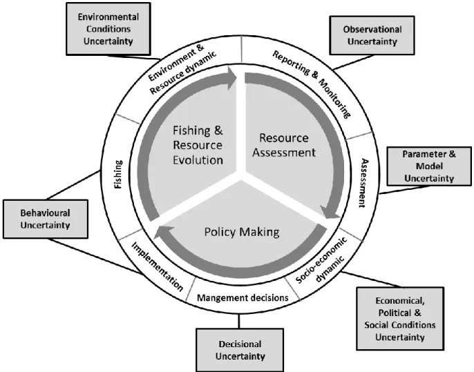
175Large uncertainty is common in most fisheries management activities. To embrace 176
uncertainties, fishery management can be viewed as an adaptive management cycle 177
(Figure 3, Walters 1986, Fulton et al. 2011) where a central fishery agency collects 178
information supporting decisions on regulations on annual or longer periods. 179
Uncertainty emerges at each step of the management cycle and can act to undermine 180
effective fishery management (Fulton et al. 2011). Previous surveys classified 181
uncertainties related to the resource dynamics, assessment and management procedure 182
and propose best practices to address those uncertainties (Figure 3, Hilborn & Peterman 183
1996; Charles 1998, Regan et al. 2002, Harwood & Stocks 2003, Peterman 2004, Hill et 184
al. 2007, Fulton et al. 2011, Link et al. 2012). Seven sources of uncertainties (sometimes 185
called error) that are important sources of risk in fisheries management have been 186
identified: uncertainties associated with environment conditions, observations, model, 187
socio-economic conditions, parameters, decisions and behaviours (adapted from 188
Hilborn & Peterman 1996, Figure 3). 189
2.2.1 Environmental conditions uncertainty 190
A major source of uncertainty in fishery systems stems from the inherent 191
unpredictability of the resource and ecosystem dynamics (Glaser et al. 2014, Planque 192
2015). In his seminal work on ecosystem resilience, Holling (1973) identified that 193
complex interactions (feedback mechanisms), stochastic and non-linear processes are 194
part of the restricting features of numerical modeling used for predictions. Without the 195
will to be exhaustive, environmental uncertainties encompass all spatio-temporal 196
variations in species and community abundance, distributions and interactions, changes 197
in life traits, periodic variability of environmental conditions or shifts in productivity 198
regimes (Link et al. 2012). For example, a typical concern in fishery management is the 199
definition of the stock recruitment relationship which is highly dependent on 200
environmental conditions and subject to random fluctuations (e.g. Fromentin et al. 201
2014). 202
2.2.2 Observational uncertainty 203
Uncertainty in observations arises from imperfect methods of observation and from 204
sampling error4. Such observation uncertainty leads to parameters estimation (or
205
inference) errors (i.e. imprecision, mis-specified parameter distributions and biased 206
parameter estimates) and structural errors (e.g. mis-specified migratory pattern and 207
stock composition). For example, the lack of fisheries-independent indices is a common 208
situation for highly migratory species (abundance indices relied mainly on catch per unit 209
effort, CPUE, Maunder & Punt 2004, Lynch et al. 2012). The logistical challenges of data 210
collection in such fishery are huge. Several sampling methods are available such as 211
tagging, larval and acoustic surveys which can provide abundance indices, but they are 212
constrained by high costs resulting in restricted spatial coverage (Leroy et al. 2015). 213
However, new methods take advantage of specific behavior of tuna species, aerial
214
surveys of tuna school counts and acoustic tagging surveys associated with fish
215
aggregating devices (FADs) are getting close to be a reliable solution to overcome this
216
4 Sampling error can be defined as the statistical differences between a sample of individuals and the population.
issue (Bauer et al. 2015, Capello et al. 2016). Mis-reporting of catch which is related to 217
illegal, unreported and unregulated (IUU) fishing is also a challenge for management of 218
highly migratory species (e.g. Fromentin et al. 2014). 219
2.2.3 Model and parameter uncertainty 220
Model and parameter uncertainties are the upshot of an incomplete, and potentially 221
misleading, representation of system dynamics (Hill 2007). Models are only abstractions 222
and there still be uncertainty about whether a given model structure (also called 223
structural uncertainty) is an appropriate representation of the system being studied. 224
Alternative model structures result in multiple model formulations that can achieve the 225
same level of fit to data (Lehuta et al. 2016). Model uncertainty can have a large impact 226
on achieving management objectives (Punt 2008). For example, even with the advent of 227
the EBFM, most of the models used in stock assessment are based on single-species age-228
structured population dynamics, ignoring important ecological interdependencies. 229
Furthermore, assessment models such as Virtual Population Analysis (VPA5) are very
230
sensitive to several assumptions about key biological dynamics such as the natural 231
mortality (Jiao et al. 2012) and selectivity patterns (Brooks et al. 2010). 232
2.2.4 Economical, political and social uncertainty 233
Uncertainty in economic, political and social conditions results from market fluctuations 234
which affect species price, as well as in fixed and variable costs of fishing effort. Such 235
variations affect expected profits and consequently the short-term dynamic behavior of 236
fishing fleets (Salas & Gaertner 2004). Consequently, the magnitude of catches might 237
vary in the short-term, affecting the population abundance. For example, in case of 238
substitutable resources on global market such as tuna species, modification in both local 239
and international political conditions and decisions (e.g. TAC in RFMOs) may also 240
constitute a source of uncertainty by altering prices and therefore economic incentives 241
(Sun et al. 2015, Guillotreau et al. 2017, Sun et al. 2017). 242
5 e.g. statistical VPA used in the International Commission for the Conservation of Atlantic Tunas (ICCAT),
2.2.5 Decisional uncertainty 243
Uncertainty in decision, changes in management objectives (resulting from an 244
unpredictable behaviour of the political authority) and the existence of multiple and 245
conflicting objectives constitute an important source of uncertainty (Anderson 1984, 246
Hilborn 2007). Political, social and economic pressures can alter management decisions 247
and lead to ignoring scientific advice claiming the argument of uncertainty in the 248
scientific advice (Rosenberg 2003, Delaney et al. 2007, Rosenberg 2007, Fromentin et al. 249
2014). For example quota reductions may not be implemented (e.g. Fromentin et al. 250
2014, Piet et al. 2010, Villasante et al. 2010, O’Leary et al. 2011). In international shared 251
fisheries6, strategic interactions play also a crucial role in the determination of common
252
management leading to cooperation between states through international arrangements 253
and institutions (e.g. RFMOs). Compared to domestic fisheries7, international fisheries
254
are subject to management difficulties mainly because of a lack of cooperation between 255
states (Munro 2004, McWhinnie 2009, Teh & Sumaila 2015). 256
2.2.6 Behavioural uncertainty 257
Uncertainty in the behaviour of resource users is the consequence of complex 258
interactions between economic and social drivers which can lead fishers to act as free-259
rider and undermine the intent of management actions (Fulton et al. 2011). Behaviour of 260
fishers concerning their spatio-temporal allocation of fishing effort to different métiers8,
261
and the reliability of catch and effort data reported, can change in an unexpected way as 262
a response of management regulations (Salas & Gaertner 2004, Vermard et al. 2012). 263
Mis-alignment between managers and users objectives has been claimed as the main 264
factor driven the uncertainty in fishers’ behaviour (Grafton et al. 2006). Divergence of 265
management intentions and response of resource users often leads to complex 266
management regulations based on an accumulation of input controls (i.e. control of 267
fishing effort, qualified of ‘band-aids’ approach, Hilborn et al. 2004). Uncertainty in the 268
behavior of resource users could be also the consequence of a lack of control or an 269
inadequate enforcement policy (Fulton et al. 2011). For example, IUU fishing can emerge 270
because of lack of control or and inadequate policy can be designed if there is no a direct 271
6 Shared fisheries refer to transboundary, straddling and highly migratory stocks. 7 Fisheries contained within one exclusive economic zone (EEZ).
link between the management lever (e.g. effort), indicator (e.g. catch) and objective (e.g. 272
constrained levels of fishing mortality, Fulton et al. 2011). 273
274
Figure 3: Schematic diagram of the rule-based adaptive management cycle and sources of uncertainties 275
that can undermine fisheries management (adapted from Fulton et al 2011). 276
3 Effect of uncertainties on optimal fishery management:
277
Does precautionary management prevail in face of
278
uncertainties?
279
3.1 Optimal fishery management problem
280Uncertainty is a central concern in fishery management, as described previously 281
complex simulation frameworks have been developed integrating ecological, economic 282
and social aspects to assess the robustness of HCRs on different kinds of uncertainty. 283
However, this approach does not allow deriving formal management rules. Feedback 284
solutions through the application of optimal control theory extensively used in fishery 285
economics studies have the ability to translate biological or ecological indicators (e.g. 286
stock) into harvest advice. The so-called ‘bang-bang’ or ‘constant-escapement’ 287
management policy finds its origin in the seminal work on feedback solutions made by 288
Clark & Munro (1975) in which the present value of the economic rent of the resource is 289
maximised by bringing the stock to an optimal level as quickly as possible. The optimal 290
escapement9 level resulting from the well-known golden rule of capital accumulation is
291
defined at the point where the internal rate of return of the stock is equal to the social 292
rate of discount (Clark & Munro 1975). Nevertheless, to achieve an efficient bang-bang 293
control, management's policy mechanisms must respond promptly and accurately 294
especially in presence of uncertainties (Roughgarden & Smith 1996). Before discussing 295
the impact of uncertainty on the optimal policy, let’s introduce the modeling framework 296
of a management problem with a single decision maker. 297
A typical discrete10 optimal dynamic management problem is defined as a social planner,
298
a hypothetical fishery manager who could be a corporation, a cooperative, a government 299
agency, or a regulatory body, someone who owns the rights to the exploitation of the fish 300
stock and which seeks to maximise the expected net present value of the resource 301
stock11. The manager decides in each period the level of a control variable (e.g. TAC) to
302
adjust the state variable (e.g. stock of fish). This decision is based on the current period 303
value function (e.g. profits from fishing) and future values which are down-weighted 304
using a discount factor. The state transition function depends on the current state and 305
control variables which ensure the Markov property. The manager’s problem can be set 306 as: 307 Subject to: 308
Where is the objective function (value function) and the 309
state transition function from period t to t+1. Each function depends on a set of 310
variables, the state variable (i.e. the stock) and control variable (i.e. the yield). The 311
9 Escapement level refers to the stock level after harvesting.
10 We only illustrate he discrete case which is sufficient to illustrate the principles involved.
11.We only focus our review on models grounded in subjective expected utility theory (SEU, see Shaw &
vectors of stochastic terms =( , ) applied on the objective function (e.g. stochastic 312
prices) or the transition function (e.g. stochastic shocks to the resource stock), vectors of 313
parameters =( , ) relating to the state transition and objective functions. Finally, δ 314
represents the discount factor. 315
Those kinds of Markov decision process (Puterman 2004) are generally solved using 316
stochastic dynamic programming techniques (Marescot et al. 2013). As highlighted in 317
Deroba & Bence (2008), stochastic dynamic programming is an efficient method for 318
defining an HCR which best meets the specified objective over a long term period. HCRs 319
can be derived both analytical and numerical, but because of their complexities most 320
fishery applications are numerical (e.g. in a deterministic framework Sandal & 321
Steinsman 1997, Grafton et al. 2000, Arnason et al. 2004). The computational cost of 322
such technique is high in face of the so called issue of ‘’the curse of dimensionality’’ 323
arising from searching over a wide range of policy strategy (Marescot et al. 2013). 324
Trade-offs between biological, economic realism and model complexity have limited 325
most fisheries applications to surplus production model. However recent studies have 326
tackled the resolution of optimal strategy in more complex settings such as the age-327
structured model (e.g. Tahvonen et al. 2017). This field of studies departs from 328
simulation-based evaluation of HCRs which consider complex modeling approach 329
evaluating the trade-offs between several indicators (e.g. studies involving MSEs). 330
Since the seminal work of Reed (1979), economic literatures have undertaken to study 331
the effect of different classes of abstracted uncertainty related to the previous 332
classification on optimal resource management policy. In the following section, we will 333
discuss the relative impacts of different classes of uncertainty on the optimal policy 334
related to the dynamic management which has been exposed. However, as pointed out 335
by Holland & Herrera (2009) findings and resulting recommendations from 336
bioeconomic models relying on optimal control theory (which found their basis in the 337
Bellman’s principle of optimality, Bellman 1957) are ambiguous or conflicting in many 338
cases. Model (structural) uncertainty relating to biological or economic assumptions has 339
been found to qualitatively and quantitatively affect the optimal policy. 340
To extract consistent and salient features of optimal policy we disregard in this section 341
the literature using complex model integrating into their model, age structuration (e.g. 342
Tahvonen et al. 2017), spatial processes (e.g. Costello & Polasky 2008), multispecies 343
interactions (e.g. Poudel & Sandal 2015) or comparison of different regulation tools (fee 344
versus quotas, e.g. Weitzman 2002). We focus our analysis on risk neutral profit 345
maximization objective12.
346
3.2 Uncertainty and precautionary management
3473.2.1 Qualitative optimal policy 348
McGough et al. (2009) provided a useful analytical solution of a general stochastic 349
fishery model on which we will stand to review the effects of uncertainties on optimal 350
policy. They concluded that the constant escapement policy is optimal under the 351
following specific structural assumptions: i) stochastic shocks affecting the stock 352
(growth) are independently and identically distributed (i.i.d.), ii) demand is perfectly 353
elastic, iii) objective implies risk neutrality and iv) marginal harvest costs are 354
independent of the quantity harvested (i.e. Schaefer's production function). Relaxing 355
one of these conditions should imply that the constant escapement policy is not optimal. 356
They demonstrated that functional assumption (linear or non-linear in state variable, 357
harvest) made on the objective function (profit function) alter the optimality of the 358
constant escapement policy. When profit exhibit a non-linear dependence on harvest, 359
the optimal policy swift toward a biomass-based rule smoothing harvest in order to 360
decrease the magnitude of the price reduction (downward slopping demand) or 361
decrease the magnitude of the cost augmentation (Cobb Douglas’ type production 362
function). Otherwise, considering a white noise (i.i.d. shocks on growth) does not affect 363
qualitatively the optimal policy, but they showed that allowing correlated environmental 364
shocks affecting the growth of the resource modify the optimal policy. The size of the 365
resource left loses its value at the expense of the size of the environmental shock which 366
provides useful information to predict future growth of the resource. 367
The constant escapement control rule is a specific policy. Catch and fishing mortality13
368
can also be used to define HCRs. The constant escapement rule involves taking all 369
biomass over some specified target level. The constant catch rule consists to harvest the 370
same biomass each year (or period) and leads to high fishing mortality when the 371
12 Or yield maximisation which is equivalent to the profit maximization objective when profit is a linear in
harvest. Furthermore, we focus on risk neutral framework and we leave the consideration about risk aversion utility function to integrate precautionary principles (Gollier et al. 2000, Chevé & Congar 2003).
biomass is at low level14, while the constant fishing mortality maintains the same fishing
372
mortality regardless of stock abundance (see supplementary materials, Appendix A). 373
From that basic HCRs, different variants have been implemented, adding more flexibility 374
related to the biomass level, to address the different weakness, such as depensatory 375
effects which can cause resource collapse. 376
We take advantage of the review of harvest policies produced by Deroba & Bence (2008) 377
to classify optimal found in the literature in 5 classes corresponding to common control 378
rules: i) constant escapement, ii) constant catch, iii) constant fishing mortality, iv) 379
biomass-based catch and v) biomass-based fishing mortality which could be assigned to 380
shock-based policy described in the theoretical result of McGough et al. (2009). In their 381
review, Deroba & Bence (2008) referred mainly on simulation-based studies which 382
analyse the performance of common HCRs relative to different objective functions15.
383
While Deroba & Bence (2008) include complex modeling framework, the general 384
qualitative findings of McGough et al. (2009) are in line with their observations (see 385
supplementary materials, Appendix B). However, the integration of the state 386
(observation) uncertainty about the size of resource seems to alter the optimality of the 387
constant escapement policy and favor a constant fishing mortality policy. 388
Therefore, based on these criteria, we reviewed the applications of optimal control 389
theory on fishery management to disentangle the qualitative effects of different classes 390
of uncertainty (Table 1 and Table 2). We compare optimal policy in the structural 391
assumptions setting define by McGough et al. (2009) by confronting what kind of control 392
rule is optimal and if greater level of uncertainty leads to more precautionary16 policy as
393
it expected under the scientific obligations to precautionary approaches. 394
3.2.2 Environmental conditions uncertainty - stochastic growth 395
3.2.2.1 Independent and identically distributed shocks 396
In surplus production biomass model, random fluctuations affecting the growth of the 397
stock are a stylised representation of the stochasticity observed in the recruitment, 398
productivity (i.e. carrying capacity) or mortality of the stock driven by environmental 399
14 Constant catch rule is defined as a depensatory policy (i.e. density independent).
15 We only keep the result based on the profit or yield maximization objective which can be linked to the
decomposition of McGough et al. (2009).
16 Precautionary means that uncertainty causes managers to choose less intensive harvest and maintain
conditions. Since the seminal work of Reed (1979), several authors have confirmed that 400
introducing stochastic growth (i.e. multiplicative i.i.d shocks in discrete setting or a 401
Wiener process in continuous setting) does not affect the optimality of the constant 402
escapement (CE) policy (Parma 1990, Sethi et al. 2005, Nostbakken 2008, Kapaun & 403
Quass 2013). However, as McGough et al. (2009) highlight the structural assumptions 404
behind this result are very restrictive. If the objective function does not respect the 405
linearity condition in harvest, the optimal policy is no longer the constant escapement 406
(Pindyck 1984, MacDonald 2002, Kugarajh et al. 2006, Nostbakken 2008, Sarkar 2009; 407
Kapaun & Quass 2013 and Kvamsdal et al. 2016). Under the non-linearity assumption, 408
the optimal HCR vary with the resource size and fit a biomass-based catch (BBC) type 409
rule defined by Deroba & Bence (2008). 410
Furthermore, increasing uncertainty surrounding the growth of the resource has a 411
different impact in term of caution if we consider linear or a non-linear objective 412
function. Nonetheless, quantitative results show only a small absolute difference. 413
Optimal feedback policies do not seem to be strongly affected by stochastic 414
environmental uncertainties. In the linear setting, increasing the uncertainty (variance 415
of the stochastic shocks) leads to an ambiguously more cautious harvest which in turn 416
preserves the resource level to higher level. When profits are non-linear in harvest the 417
resulting cautious of HCR is ambiguous. McDonald et al. (2002), Kugarajh et al. (2006) 418
and Kvamsdal et al. (2016) found that increasing uncertainty has the same effect that 419
increasing the discount rate in the deterministic case especially at low stock level. The 420
resulting optimal HCR is, therefore, more aggressive when uncertainty is high and 421
resource is scarce. However, their logistic growth model which includes a specific 422
depensation response creates an incentive to fish down the resource when the stock 423
falls below the critical depensation level. In such case, the stock will be unable to 424
recover. When the depensation assumption is relaxed, Sarkar et al. (2009) found that the 425
optimal harvest (HCR) size is a decreasing function of the growth uncertainty. Pindyck 426
(1984) has generalized the condition in which uncertainty lead to more or less cautious 427
harvesting behaviour when stochasticity is included in a non-linear model. Growth 428
fluctuations reduce the value of the stock, and because their variance is an increasing 429
function of the stock level, there is an incentive to reduce the stock level by harvesting 430
faster. Growth fluctuations also increase in average harvesting costs and create an 431
incentive to increase harvest rate. If we consider a fixed harvest rate, the expected 432
growth rate of the stock decreased which in turn reduces the harvest rate. Therefore, 433
Pindyck concludes that the effect of uncertainty on the feedback control rule is 434
indeterminate. Kapaun & Quass (2013) came to a similar conclusion in a discrete setting 435
assuming a convex cost function and infinitely elastic demand. They demonstrated that 436
the optimal HCR could be higher or lower than in the deterministic setting. 437
A special case of non-linear objective function concerns convex profits. This situation 438
typically involves schooling fisheries which face concave cost functions. When fish 439
presents schooling behaviours, as long as fishermen have the ability to locate the schools 440
harvest does not depend on the size of the resource. This structural assumption yields 441
incentives to fish down the stock at low level increasing the risk of collapse. 442
Furthermore, this assumption turns the HCR into a pulse-fishing type which induces to 443
harvest a lot above a threshold and then let the stock growth (Maroto & Moran 2008, 444
Maroto et al. 2012). Da Rocha et al. (2014) investigated the effect of growth uncertainty 445
when increasing returns are considering. They confirmed that convex profits conduct to 446
pulse fishing, but increasing growth uncertainty tends to fit a constant escapement 447
policy. 448
Overcapacity is widely recognized as a major problem affecting world fisheries. Even in 449
a regulated fishery, overcapacity in fishing fleets in response to (temporarily or 450
cyclical)17 positive rents is a major impediment to achieving economically productive
451
fisheries (Beddington et al. 2007). Most of the studies ignore the cost of investing in 452
fishing vessels by considering the capital as perfectly malleable. Introducing costly 453
capital adjustment turns the optimal policy into a biomass-based catch type. When the 454
objective function is linear in harvest, uncertainty in growth leads in most case to a more 455
precautionary harvest of the resource (e.g. Charles and Munroe 1985). However, when 456
stocks are fast growing and capital are low cost, investment in large fleet which offers 457
the opportunity to take advantage of positive recruitments events (positive shocks), 458
becomes a reliable strategy. This result holds even if we consider the objective function 459
to be non-linear in harvest (Poudel et al. 2015). Costly capital adjustment can also be 460
linked to policy adjustment18 (e.g. TAC adjustment). When a resource fluctuates
461
randomly, biomass-based or constant escapement HCR increases variability in catch to 462
17 Overcapacity can result from several sources such as periodic fluctuation of fish abundance (e.g. Fréon
et al. 2008), use of subsidies (e.g. Clark et al. 2004), fluctuation of variable costs (e.g. fuel price) or directly fish price which affect the profitability of the fishery (e.g. Sumaila et al. 2008). The high profitability of the initial phase of a developing fishery is typical case of overcapitalisation.
reflect environmental variation (Deroba & Bence 2008). A trade-off between more or 463
less responsive approaches to environmental variations which can lead to more or less 464
precautionary harvest depends on the linearity assumption of the objective function and 465
the forms of policy costs (Boettiger et al. 2016, Ryan et al. 2017). 466
3.2.2.2 Correlated and cyclical variations 467
Considering that environmental fluctuations are serially uncorrelated is a strong 468
assumption. Many observations showed that recruitment is serially correlated induced 469
by environmental signals (e.g. Koster 2005). Furthermore, growth rates of fish stocks 470
have been shown to be non-stationary. Cyclical environmental variations over large 471
range of temporal scales independently of fishing activity have been shown to induce 472
fluctuations of fish stock. For example, several studies have shown the influence of large 473
scale climatic variations such as the El Nino Southern Oscillation (e.g. Lehodey et al. 474
1997) or long term trend in physical factors such as the temperature (e.g. Ravier &
475
Fromentin 2004). 476
McGough et al. (2009) demonstrated that when environmental fluctuations are 477
correlated or cyclical are considered the optimal policy becomes sensitive to 478
environmental shocks which fit a biomass-based fishing mortality (BBF) HCR. This 479
result is in line with studies which include correlated or cyclical variations of fish stock 480
growth (e.g. Parma 1990, Walters & Parma 1996, Singh et al. 2006 and Carson et al. 481
2009). When fluctuations are cyclical, the optimal HCR followed closely environment 482
cycles with lower escapement when conditions are poor and higher when conditions are 483
good (Parma 1990, Walters & Parma 1996 and Carson et al. 2009). This investment 484
behavior taking advantage of good environmental condition to invest in the resource 485
reinforces recruitment fluctuations. Singh et al. (2006) found close results with a model 486
included simultaneously correlated random stock growth and costly capital adjustment 487
with a non-linear objective function. Under these assumptions, they showed that optimal 488
HCR implies to build up the fleet when environmental conditions are good (positive 489
serial correlation) in anticipation of higher future catch levels and decrease fleet when 490
conditions are poor. 491
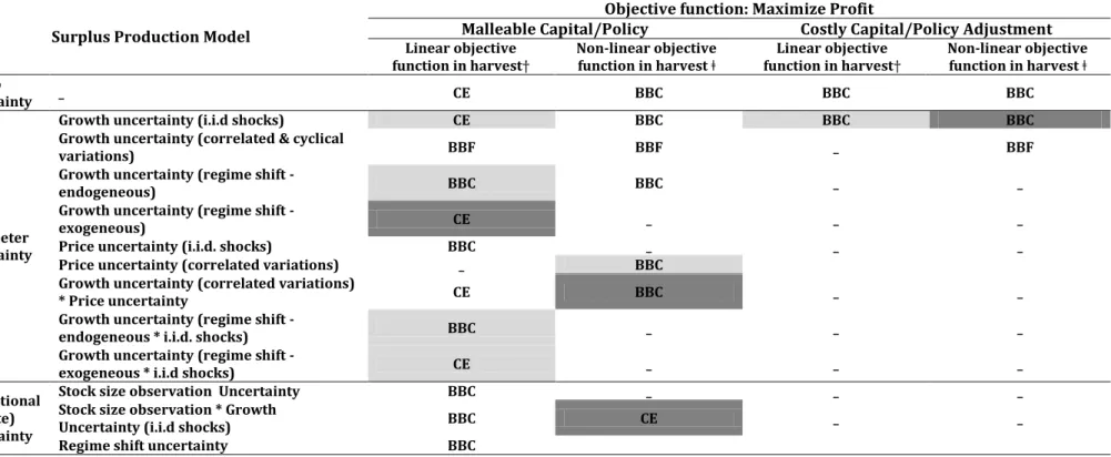
Table 1: Optimal HCRs policy and precautionary behaviour compared to the deterministic case based on a review of the available literature. 492
Surplus Production Model
Objective function: Maximize Profit
Malleable Capital/Policy Costly Capital/Policy Adjustment
Linear objective
function in harvest† Non-linear objective function in harvest ǂ function in harvest† Linear objective Non-linear objective function in harvest ǂ No
uncertainty _ CE BBC BBC BBC
Parameter uncertainty
Growth uncertainty (i.i.d shocks) CE BBC BBC BBC
Growth uncertainty (correlated & cyclical
variations) BBF BBF _ BBF
Growth uncertainty (regime shift -
endogeneous) BBC BBC _ _
Growth uncertainty (regime shift -
exogeneous) CE _ _ _
Price uncertainty (i.i.d. shocks) BBC _ _ _
Price uncertainty (correlated variations) _ BBC
Growth uncertainty (correlated variations)
* Price uncertainty CE BBC _ _
Growth uncertainty (regime shift -
endogeneous * i.i.d. shocks) BBC _ _ _
Growth uncertainty (regime shift -
exogeneous * i.i.d shocks) CE _ _ _
Observational (State) Uncertainty
Stock size observation Uncertainty BBC _ _ _
Stock size observation * Growth
Uncertainty (i.i.d shocks) BBC CE _ _
Regime shift uncertainty BBC
CE : Constant Escapement policy BBC: Biomass-based catch policy
BBF: Biomass-based fishing mortality policy
† Infinitely elastic demand associated with Schaefer’s type production function or yield maximization. ǂ Downward slopping demand or/and Cobb Douglas’ type production function non-linear in harvest. : More precautionary optimal policy
: Less precautionary optimal policy : Ambiguous effect or no effect
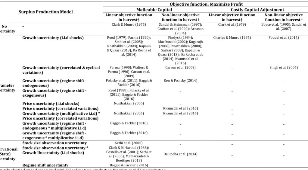
Table 2: References used for the construction of Table 1. 493
Surplus Production Model
Objective function: Maximize Profit
Malleable Capital Costly Capital Adjustment
Linear objective function
in harvest† Non-linear objective function in harvest ǂ Linear objective function in harvest† Non-linear objective function in harvest ǂ No
uncertainty
_ Clark & Munro (1975) Sandal & Steinsman (1997);
Grafton et al. (2000); Arnason (2004)
Clark et al. (1979) Boyce et al. (1995); Sandal et al. (2007)
Parameter uncertainty
Growth uncertainty (i.i.d shocks) Reed (1979); Parma (1990); Sethi et al. (2005); Nostbakken (2008); Kapaun & Quaas (2013); Da Rocha et
al. (2014)
Pindyck (1984); MacDonald (2002); Kugarajh
(2006); Nostbakken (2008); Sarkar (2009); Kapaun & Quass (2013); Da Rocha et al.
(2014); Kvamsdal et al. (2016)
Charles & Munro (1985) Poudel et al. (2015)
Growth uncertainty (correlated & cyclical variations)
Parma (1990); Walters & Parma (1996); Carson et al.
(2009)
Carson et al. (2009) _ Singh et al. (2006)
Growth uncertainty (regime shift - endogeneous)
Polasky et al. (2011); Baggio&
Fackler (2016) Ren & Poalsky (2014) _ _
Growth uncertainty (regime shift - exogeneous)
Reed (1988); Polasky et al. (2011); Baggio & Fackler
(2016)
_ _ _
Price uncertainty (i.i.d shocks) Nostbakken (2006) _ _
Price uncertainty (correlated variations) Kvamsdal et al. (2016) _
Growth uncertainty (multiplicative i.i.d) * Price uncertainty (correlated variations)
Nostbakken (2006) Kvamsdal et al. (2016) _ _
Growth uncertainty (regime shift - endogeneous * multiplicative i.i.d)
Baggio & Fackler (2016) _ _ _
Growth uncertainty (regime shift - exogeneous * multiplicative i.i.d)
Baggio & Fackler (2016) _ _ _
Observational (State) Uncertainty
Stock size observation uncertainty Sethi et al. (2005) _ _ _
Stock size observation uncertanty * Growth Uncertainty (i.i.d shocks)
Clark & Kirkwood (1986); Costello et al. (2001); Sethi et
al. (2005); Memarzadeh & Boettiger (2018)
Da Rocha et al. (2014) _ _
Regime shift uncertainty Baggio & Fackler. (2016)
† Infinitely elastic demand associated with Schaefer’s type production function or yield maximization. ǂ Downward slopping demand or/and Cobb Douglas’ type production function non-linear in harvest.
3.2.2.3 Regime shifts 494
Complex interaction and dynamic in fishery systems may induce sudden and drastic 495
switch between contrasting stable states (Scheffer et al. 2001, Folke et al. 2004). 496
Exogenous environmental shocks and fishing activity may trigger a regime shift from 497
high to low productive regimes or irreversible collapse of populations (review in Jiao 498
2009 and Kraberg et al. 2011). Catastrophic shifts such as fishery collapses have been 499
mainly attributed to overfishing as a result of economic factors and mismanagement, but 500
environmental stochasticity associated with depensatory mechanism may also be a 501
cause of fisheries collapse (Mullon et al. 2005). 502
Regime shifts pose difficult challenges for management (Crépin et al. 2012) which 503
depend whether the dominant factors are exogenously and/or endogenously 504
determined as well as on their severity and irreversibility (catastrophic consequences or 505
shift in productivity). The severity criterion appears to be less significant in the 506
determination of the precautionary of the optimal HCR. Therefore, we dissociate studies 507
on the basis of the likelihood of the shift (change in the stock growth function) is
508
exogenous or a function of management actions (e.g. TACs).
509
Reed (1988) seminal work applied a general surplus production model with a linear
510
objective function in harvest and stochastic exogenous and endogenous irreversible
511
regime shift (catastrophic collapse consequences). Uncertain exogenous shift reduces 512
the future value of the resource which gives incentives to harvest the resource in the 513
current period resulting in more aggressive HCR. However, endogenously driven shifts 514
result in more precautionary harvest which depends on how the shifting probability 515
increases as resource level decreases (density-dependent effect) compared to the 516
density-independent nature of the hazard rate function (density-independent effect). 517
When the population is able to recover after collapse (reversible shift), the resulting 518
HCR becomes more aggressive because of the reduction of the density-dependent effect. 519
Polasky et al. (2011) generalized these results considering two kinds of shifts:
520
catastrophic collapse or change in system dynamic (reduced growth). Their findings 521
confirmed Reed’s outcomes, when the risk is endogenous the cautious of the resulting 522
HCR depends on the severity of the consequence of the shift which gives more weight to 523
the density-independent effect. If the shift is reversible or implies non-catastrophic 524
consequence, the resulting HCR is more cautious. On the contrary, when the shift is 525
irreversible and lead to stock collapse the resulting HCR is ambiguous depending on 526
which of the opposite density-dependent and independent effects dominate. Ren & 527
Polasky (2014) examined the optimal management problem with a general utility 528
function rather than a linear function. They demonstrated that the shape of the utility 529
function considerably affects the optimal HCR which may become more or less 530
precautionary depending on the relative magnitudes of two kinds of effects acting in 531
opposite directions. Concomitantly, a regime shift lowers the future profit from the 532
fishery which reduces the profitability of the investment in the resource. Finally, Baggio
533
& Fackler (2016) extended the previous model by considering stochastic shocks (i.i.d.)
534
and non-catastrophic reversible shifts affecting growth of the resource. Their numerical
535
analysis confirmed the analytical results from Polasky et al. (2011) emphasising the
536
influence of growth stochasticity on the cautious of the optimal HCR. They also showed 537
that the endogenous switching probability changes the optimal policy to a biomass-538
based catch type with a far more precautionary strategy. In summary, the degree of
539
contrast and resilience (reversibility between states) as well as volatility of the resource
540
fluctuations has important impact on optimal policy.
541
3.2.3 Economical, political and social uncertainty - Stochastic price 542
Uncertainties related to economic conditions have been limited to market fluctuations 543
affecting fish price (Nostbakken 2006, Kvamsdal et al. 2016). Price uncertainty has been 544
found to play only a minor role in the determination of the optimal HCR. However, the 545
optimal policy is no longer a constant escapement. Kvamsdal et al. (2016) described a 546
smooth harvest policy as a function of stock size and price with a non-linear objective 547
function. Additionally, although price uncertainty has only a minor effect, volatility in 548
price leads to relatively more cautious harvest which buffers the increasing price effect 549
with the scarcity of the resource. 550
3.2.4 Observational uncertainty – Uncertain states 551
Perfect information has been assumed in most studies, however, fishery management 552
relies on indirect observations of fish stocks which are subject to high level of 553
uncertainties. Additionally, assessments methods are imperfect and subject to many 554
sources of bias. Relaxing the perfect observation assumption change considerably the 555
optimal HCRs and no longer fit Markov decision process framework needed to employ 556
standard stochastic dynamic programming method (Fackler & Pacifi 2014). 557
Clark & Kirkwood (1986) and Sethi et al. (2005) tackled the stock measurement 558
uncertainty problem and showed that the optimal HCR is less conservative than the 559
deterministic solution. Moreover, they found that the optimal policy becomes sensitive 560
to stock size (biomass-based catch policy) when measurement errors are introduced. In 561
the case where multiple uncertainties are confronted, measurement uncertainty has the 562
largest impact on the determination of the optimal HCR. Memarzadeh & Boettiger 563
(2018) argued that these counterintuitive results are supported by means of a 564
simplification which ensures that the transition probability between states is 565
independent of all previous states. They demonstrated through the implementation of a 566
partially observed Markov decision process19 approach which relaxed the full
567
observability assumption of the system's state that more conservative policy is optimal. 568
While state uncertainties concern primarily the size of the resource, in more complex 569
setting such as regime shift dynamics, the current regime may not be directly observed. 570
Using a partially a partially observed Markov decision approach Baggio & Fackler (2014) 571
showed that policy adjustment depends on the weight of belief in a given regime. 572
Additionally, optimal policy tends to be more or less precautionary depending on the 573
belief state. Past information are determinant in the definition the optimal policy, thus 574
anticipating future conditions may also affect the optimal HCR. Costello et al. (2001) 575
investigated the impacts of growth fluctuations shocks (i.i.d.) when an uncertain forecast 576
of environmental shocks is available. When new information is available, the optimal 577
escapement is no longer constant but varies with the shocks prevision and increases 578
substantially the profits. 579
3.2.5 Model and parameter uncertainty 580
Structural uncertainty arises when a system is imperfectly understood and represented 581
(Williams 2011). As we discuss previously, the choice of optimal HCR depends critically 582
on structural assumptions. The selection of an objective function and appropriate 583
uncertainties which represent the system determined the class and the precautionary of 584
the optimal HCR. The central objective in adaptive management is learning, which 585
19 Extension of Markov decision process in which unobservable state variables are replaced by a belief
should occur through the adjustments of decision making allowing by new information 586
(Walters 1986, Williams 2011). Model and parameter uncertainties can be addressed by 587
new modeling frameworks which extend the standard Markov decision process using 588
Bayes rule. Unknown parameters or functional forms of the system are replaced by 589
belief distributions updating through time and new information gathered (Fackler 2014, 590
Fackler & Pacifi 2014, Williams 2016, LaRiviere et al. 2017). Memarzadeh & Boettiger 591
(2018) are among the first implementations of adaptive management to renewable 592
resource management introducing model, parameters and observation uncertainties. 593
This promising framework should be a serious candidate to compete with simulation-594
based approaches such as MSE. However, such approaches still need to select pertinent 595
structural assumptions and uncertainties to include as potential candidate to 596
characterize the system. 597
Along with the development of modeling methods to address adaptive management, 598
more complex model such as stochastic age-structured model has been studied. 599
Bioeconomic studies surveyed have been criticised for being too simple to sustain 600
management guidelines. Trade-offs between simple and more complex models such as 601
age-structured are central when we evaluate the cost-benefits of using models for 602
management which in turn reduce ease of learning and communication. However only 603
few studies have undertaken to study uncertainties effect in age structured model 604
(Holden & Conrad 2015, Tahvonen et al. 2017). They found that such as for surplus 605
biomass model, the addition of random recruitment fluctuations (i.i.d. shocks) does not 606
affect strongly the optimal HCR. 607
3.3 Decisional uncertainty- the case of shared fisheries management
608Our review builds on the studies where decision making relied on a unique hypothetical 609
fishery manager who could be a corporation, a cooperative, a government agency, or a 610
regulatory body. However, many fish stocks are not solely distributed within a single 611
exclusive economic zone (EEZ). Thus, the assumption of a single manager or a 612
cooperative organization holds the responsibility of the decision making is no longer 613
acceptable. Shared fish stocks (Munro et al. 2004, Munro 2007) are a special case which 614
causes particular strategic management problems (McWhinnie 2009). Optimal 615
management studies leave aside the question of how stakeholders’ strategic 616
considerations are influenced by uncertainties. Two kinds of uncertainties arise in social 617
dilemmas20 such as shared fisheries, social and environmental uncertainty (van Dijk et
618
al. 2004). When we consider a group of stakeholders on which relies a common decision, 619
social uncertainty refers to the individual uncertainty about what their fellow group 620
members will decide. Whereas, environmental uncertainty relates to the characteristic 621
of the dilemma which defines the fishery system, the number of stakeholders involved 622
and also uncertainties related to fishery management previously introduced. A central 623
question in shared fisheries is, therefore, would interaction between social and 624
environmental uncertainty lead to more precautionary or to more aggressive 625
management. The economics of shared fisheries is anchored on game theory as the
626
management of internationally shared fish stocks involves the strategic interaction
627
between several countries. Several approaches have been used useful to understand
628
cooperation in such context, but two main strands of game literature applying to shared
629
fisheries can be considered, cooperative and non-cooperative dynamic or coalition
630
games (reviews in Hannesson 2011, Miller et al. 2013, Pintasssilgo et al. 2015).
Non-631
cooperative games involve competition between stakeholders in which only self-632
enforcing (e.g. through threats) cooperation are possible, while cooperative games, a 633
priori, suppose that cooperative behaviours are enforced through external binding 634
agreements (e.g. International Fisheries Agreements, IFA). Early game theory studies 635
showed that competitive behaviours lead to the well-known the tragedy of the commons 636
(Hardin 1968), while a joint exploitation of the resources is equivalent to the optimal 637
management under the sole manager hypothesis (Munro 1979). However, only a few 638
studies integrated uncertainty or incomplete information21 in the analysis of strategic
639
interaction in shared fisheries. Stochastic models22 provide key information to studies
640
anticipate how shocks and potential regime shifts in the system may affect the 641
cooperative solution and its stability compared to the sole ownership theoretical case. In 642
various settings included growth (recruitment), migration fluctuations, imperfect 643
monitoring or potential regime shifts, several works have shown ambiguous results of 644
20 Social dilemma refers to a situation where a group members experience a conflict between their
personal interests and the interests of the group to which they belong.
21 Imperfect information can concern player actions, e.g. monitoring of harvests (Laukkanen 2003, Tarui et
al. 2008) or the state of the system (Laukkanen 2003).
22 Stochastic models concern growth (recruitment) uncertainty in fish-war game type (Antoniadou et al.
2013, Diekert & Nieminem 2017) or in sequential game (Laukkanen 2003), the migration pattern of fish stock under climate change in fish-wars game (McKelvey et al. 2003), potential regime shifts in productivity or collapse which are exogenous (Fesselmeyer & Santugini 2013, Sakamoto 2014, Miller & Nkuiya 2016), or endogenous (Sakamoto 2014, Miller & Nkuiya 2016) in fish-wars game.