HAL Id: hal-00969339
https://hal.archives-ouvertes.fr/hal-00969339
Submitted on 2 Apr 2014
HAL is a multi-disciplinary open access
archive for the deposit and dissemination of
sci-entific research documents, whether they are
pub-lished or not. The documents may come from
teaching and research institutions in France or
abroad, or from public or private research centers.
L’archive ouverte pluridisciplinaire HAL, est
destinée au dépôt et à la diffusion de documents
scientifiques de niveau recherche, publiés ou non,
émanant des établissements d’enseignement et de
recherche français ou étrangers, des laboratoires
publics ou privés.
Supervisory hybrid model predictive control for voltage
stability of power networks
Rudy R. Negenborn, Giovanni Beccuti, Turhan Demiray, Sylvain Leirens,
Gilney Damm, Bart de Schutter, Manfred Morari
To cite this version:
Rudy R. Negenborn, Giovanni Beccuti, Turhan Demiray, Sylvain Leirens, Gilney Damm, et al..
Supervisory hybrid model predictive control for voltage stability of power networks.
Ameri-can Control Conference (ACC 2007), Jul 2007, New York, NY, United States.
pp.5444–5449,
Supervisory hybrid model predictive control
for voltage stability of power networks
R.R. Negenborn, A.G. Beccuti, T. Demiray, S. Leirens, G. Damm, B. De Schutter, M. Morari
Abstract— Emergency voltage control problems in electric
power networks have stimulated the interest for the imple-mentation of online optimal control techniques. Briefly stated, voltage instability stems from the attempt of load dynamics to restore power consumption beyond the capability of the transmission and generation system. Typically, this situation occurs after the outage of one or more components in the network, such that the system cannot satisfy the load demand with the given inputs at a physically sustainable voltage profile. For a particular network, a supervisory control strategy based on model predictive control is proposed, which provides at discrete time steps inputs and set-points to lower-layer primary controllers based on the predicted behavior of a model featuring hybrid dynamics of the loads and the generation system.
I. INTRODUCTION
Huge problems in the US and Canada [1], Italy, and The Netherlands due to power outages have shown the crucial role of a reliable operation of electricity distribution and transmission networks. A reliable and efficient operation of these networks is not only of paramount importance when these electricity systems are pressed to their limits of its performance, but also under regular operating conditions. Due to the deregulation in the European electricity market, the number and variety of actors increases. This number will even further increase as also large-scale industrial suppliers and small-scale individual households (via solar energy or wind energy installations) will start to feed electricity into the network [2]. With this increasing complexity faults and disturbances causing voltage instabilities are likely to occur more frequently.
In general, the behavior of power systems is characterized by complex interactions between continuous dynamics and discrete events, i.e., power systems exhibit hybrid behavior. Components such as generators and loads drive the con-tinuous dynamic behavior. They obey physical laws, and are usually represented by coupled differential and algebraic equations. Discrete events or discrete inputs cause discrete behavior through, e.g., breaking down or connecting of a transmission line, saturation effects in automatic voltage reg-ulators and power system stabilizers, on or off switching of R.R. Negenborn and B. De Schutter are with the Delft Center for Systems and Control, Delft University of Technology, Delft, The Nether-lands,[email protected], [email protected]. A.G. Beccuti and M. Morari are with the Automatic Control Laboratory, ETH Z¨urich, Switzerland,{beccuti,morari}@control.ee.ethz.ch. T. Demiray is with the Power Systems Laboratory, ETH Z¨urich, Switzer-land, [email protected]. S. Leirens is with the Auto-matic Control of Hybrid Systems group, Sup´elec, Rennes, France,
[email protected]. G. Damm is with the Laboratoire In-formatique, Biologie Int´egrative et Syst`emes Complexes, Universit´e d’Evry-Val d’Essonne, Evry, France,[email protected].
generators, connecting or disconnecting of loads, changing of transformer ratio settings, and connecting or disconnecting of capacitor banks; seasonal variations can also cause changes in power production capabilities as well as consumption and can modify the direction of power flows and thus cause switching behavior. The networks moreover typically span a wide range of time scales and large geographical areas.
To control such complex systems, hierarchical control in which control takes place at different layers based on space and/or time division is necessary [3]. The controllers at the lowest layer act directly on the actuators of the physical system, employing faster and more localized control. Higher-layer controllers supervise controllers of lower Higher-layers by pro-viding set-points or specifying constraints, employing slower and more overall control. The task of a higher layer is to steer the underlying layer in such a way that the performance of the physical system is optimal in some sense. Traditionally in hierarchical control, a layer either only provides continuous or only discrete values to a different layer. In the approach we propose, both continuous and discrete values are dealt with in an integrated way, i.e., we consider a hybrid approach.
The particular control problem we are dealing with is voltage stability after disturbances. After a disturbance, e.g., breaking of a transmission line, the generation and transmis-sion network may not have sufficient capacity to provide the loads with power; voltage instability may be the result. Con-trol actions have to be chosen that minimize negative effects of this voltage instability. Traditionally, offline static stability studies are carried out in order to avert the occurrence of voltage instability. The approach we propose is an application of online control that takes into account both the inherent temporal dynamics and that determines the most appropriate control sequence required to reach an acceptable and secure operating point. We consider a scheme used by a higher-layer controller that controls a power network to determine both discrete and continuous set-points for lower-layer controllers in such a way that negative effects due to voltage instability after disturbances are minimized. We hereby assume that a lower layer that accepts set-points at discrete time steps is already present.
This paper is organized as follows. In Section II we introduce the power network and the lowest layer of control that we consider. In Section III we introduce the voltage control problem and the objectives. In Section IV we present a control strategy for the higher layer based on model predictive control. Section V contains simulation results obtained on the considered power network.
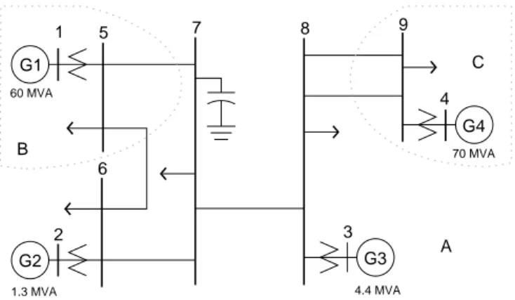
A 8 7 3 4.4 MVA C 70 MVA 4 1.3 MVA B 60 MVA 1 6 5 2 9 G4 G3 G2 G1
Fig. 1. Graphical representation of the IEEE 9-bus Anderson-Farmer network.
II. POWER NETWORK SYSTEM
A. Physical network
The case study under consideration is the 9 bus Anderson-Farmer network [4], depicted in Fig. 1, taken from the Dynamical Systems Benchmark Library1, whereto the reader
is referred for an exhaustive description. B. Components of the network
The considered network consists of 4 generators G1, G2, G3 and G4 (shown with their nominal apparent power
ratings) feeding the static loads at buses5 through 9, where G1 and G4 and the loads connected to buses 5 and 9 are
the aggregate representations for neighboring generators and loads. The synchronous machines are connected to the grid via lossless step-up transformers featuring a fixed turns ratio; a capacitor bank at node7 provides additional reactive power
to the system. The following list contains more details:
• Generators: Generators G2 and G3 represent single
physical machines, whereas G1 and G4 denote the
aggregate generators comprising several physical units. Therefore, G2and G3are described by a detailed
sixth-order model [5] including the mechanical equations and the electrical transient and sub-transient dynamics, whereas G1 and G4 are described by second-order
mechanical dynamics [5].
• Loads: The employed static loads comprise voltage
dependent and constant impedance types [6]. The loads are described with following classical formulation in terms of active and reactive power
Ph= shP0hvhα (1a) Qh= shQ0hvαh, (1b)
where h∈ {5, 6, 7, 8, 9}, vhis the voltage of bus h, P0h
(Q0h) is the active (reactive) power steady-state value at
node h, and sh ∈ {0, 0.02, . . . , 0.98, 1} per unit (p.u.)
represents the discrete load shedding factor applied to a load to relieve the strain of the power demand on the
1URL:http://psdyn.ece.wisc.edu/IEEEbenchmarks/
system. Voltage dependent loads correspond to α= 1
and constant impedance loads to α= 2.
• Capacitor bank: The capacitor bank locally stabilizes
bus voltages by injecting additional reactive power into the grid. It is represented as a (negative) purely reactive load of type (1b) with α = 2 and thus describes a
switched shunt capacitor.
• Transmission lines: The transmission lines between the
buses and components transfer the power from one location to another. The lines are represented by the
π model for transmission lines [5].
C. Primary control layer
In the network there is a primary, lower-layer, control layer that locally regulates power flows and voltage levels at the bus terminals of generators. Fig. 2 shows a schematic representation of the local controllers’ principle of operation. Feedback variables and corrective actions are depicted for each component [5]. The primary control layer consists of the following:
• Turbine governors: All generators feature a turbine
governor (TG) controlling the mechanical power Pm
acting on the shaft of the machine in order to satisfy the active power demand of the network and maintain the desired frequency ωref= 60 Hz. The TGs act on a
time scale of tens of seconds.
• Automatic voltage regulators: All generators feature an
automatic voltage regulator (AVR) maintaining the level of the excitation field Efd in the rotor windings at the
value required to keep the bus (stator) voltage close to the desired set-point. Saturation is included in the AVR to account for the maximum allowable current in the excitation system, i.e., Efdhas an upper limit value Emaxand a lower limit value Emin. Once a machine has
reached its saturation limit it cannot produce additional reactive power and can therefore no longer participate in sustaining the voltages in the network [5]. The AVR voltage reference ri of generator i, i∈ {1, 2, 3, 4}, can
be set in the range0.9 − 1.1 p.u. with steps of 0.01 p.u.
The AVRs act on a time scale of seconds.
v, i v v E P T − ω + v + − + ref,PSS ref ω fd m (network) ref 60 m = Hz damping torque Control input
Regulates mechanical torque to achieve active power balance
Gives a signal that increases Feeds field winding to create rotor flux
and control node voltage v
Governor Turbine
Turbine Synchronous Machine
Regulator Automatic Voltage
Power System Stabilizer
• Power system stabilizers: Generators G2and G3feature
a power system stabilizer (PSS) eliminating the pres-ence of unwanted rotor oscillations by measuring the rotational speed ω and adding a corrective factor vref,PSS
to the bus terminals’ voltage reference vref. Generators G1and G4feature no power system stabilizer since the
faster dynamics related to the rotor oscillations are not present in the related model equations. The PSSs act on a time scale of tenths of seconds.
D. Controls available to a higher control layer
Given the description of the network and the primary control layer, there is a number of controls available to a higher control layer in the form of set-point and reference settings. In particular the following can be adjusted:
• the voltage references for the AVRs; • the mechanical power set-point for the TGs; • the reference frequency for the TGs and PSSs; • the amount of load to shed;
• the amount of capacitor banks to connect to the grid.
Depending on the particular control problem a higher-layer controller will adjust the values of these controls. In particu-lar for the problem at hand the amount of load shed (defined by the variables sh) and the set-points of the AVRs (defined
by the variables ri) will be taken as the available controls.
III. EMERGENCY VOLTAGE CONTROL
A major source of power outages is voltage instability [7]. Voltage instability in general stems from the attempt of load dynamics to restore power consumption beyond the capability of the combined transmission and generation system. Typically, the capability is exceeded following the outage of one or more components in the network, such that the system cannot satisfy the load demand with the given inputs at a physically sustainable voltage profile in the network.
The control problem involves the case of emergency voltage regulation, in which the power system is initially in steady-state operation and subsequently subjected to a fault, modeled as the partial or total outage of a line. Due to the reduced transmission capacity of the network the requested load demand together with the given system configuration place the grid under an excessive amount of strain, so that corrective actions are required to avoid that the induced transients drive the system to collapse or cause unwanted and hazardous sustained oscillations. More specifically, the control objectives are:
1) Maintain the voltages between 0.9 and 1.1 p.u., i.e.,
sufficiently close to nominal values to ensure a safe operation of the system by keeping it sufficiently dis-tant from low voltages, which may lead to a collapse. 2) Effectively achieve a steady-state point of operation, while minimizing switching of the control inputs so that a constant and appropriate set of input values is ultimately applied to the power grid.
For this second objective, in particular the option of shedding load is to be avoided unless absolutely necessary in order to
fulfill the primary objective, as load shedding is the most disruptive countermeasure available.
IV. MODELPREDICTIVECONTROL
Model Predictive Control (MPC) [8], [9] has been tra-ditionally employed in the process industry and has shown promising performance also for a variety of other control problems [10]. The control action is obtained at each time step by minimizing an objective function over a finite horizon subject to the equations of the employed prediction model and the operational constraints, e.g., on inputs. The control problem is solved in a receding horizon fashion. The major advantage of MPC is its straight-forward design procedure. Given a model of the system, hard constraints can be incorporated directly as inequalities and one only needs to set up an objective function reflecting the control aim; soft constraints can also be accounted for in the objective by using penalties for violations.
A. Derivation of the prediction model
The performance of a predictive controller relies for a large part on the accuracy of the prediction model of the system. The prediction model has to describe well how the inputs affect the system behavior. Ideally a perfect model of the system would be used; however, such a perfect model can be very complex, thus making the optimization procedure in the controller slow. Instead, an approximation is used. If this approximation fits in a suitable form, relatively efficient optimization techniques can be used to determine the controls (e.g., linear or mixed-integer linear programming).
In order for the higher-layer controller that we are design-ing to meet its control objectives, it has to be able to predict how set-point changes influence the dynamics of the network. Therefore, the controller uses a model that includes both a representation of the physical network and a representation of the primary control layer.
The network, including the primary control layer, is ex-pressed [5] as a system of differential-algebraic equations (DAE)
˙x = f (x, u, v) (2a)
0 = g(x, u, v) (2b) where the state variables x are the generator dynamic variables, u denotes the system inputs, and the algebraic output variables v are the bus voltage magnitudes. The dif-ferential equations (2a) describe the synchronous machines and related primary controllers; the algebraic equations (2b) describe the classic load flow equations. See for the tech-nical details on the power system models used the location specified in footnote 1.
Determining the evolution of the network given an initial state and input trajectory over the horizon thus requires the solution of this DAE. Solving DAEs in general is a complex task, in particular when dynamics of different time scales are present, as is the case for the power systems. Variable step size methods, e.g., DASSL [11], are suitable for these cases, since they automatically choose a larger step size
when no fast dynamics are present, and a smaller step size when they are [12]. However, using these methods inside the optimization procedure of the MPC controller could be very time-consuming and could thus result in very slow control. Therefore, such a DAE model is not directly suitable as prediction model.
Instead of taking the continuous-time DAE as prediction model, we consider a discrete-time linearized model derived from this DAE. At each discrete sampling instant kTs the
continuous-time linearization of (2a) and (2b) around x0 = x(k), u0= u(k − 1), can be written as
˙x = Acx+ Bcu+ Fc v= Ccx+ Dcu+ Gc, where Ac =∂f∂x+∂f∂v(−∂g∂v)−1(∂x∂g), Bc = ∂f∂u+∂f∂v(−∂g∂v)−1 ∂g∂u Cc = (−∂g∂v)−1 ∂g∂x, Dc = (−∂g∂v)−1 ∂g∂u Fc= − ∂f ∂v(− ∂g ∂v) −1 (∂g ∂xx0+ ∂g ∂uu0+ ∂g ∂vv0− g(x0, u0, v0)) − (∂f ∂xx0+ ∂f ∂uu0+ ∂f ∂vv0− f (x0, u0, v0)) Gc= −(− ∂g ∂v) −1(∂g ∂xx0+ ∂g ∂uu0+ ∂g ∂vv0− g(x0, u0, v0))
when ∂g∂v is invertible, which is typically the case for power networks. The required Jacobians can either be derived analytically [13] or computed numerically. For the sake of simplicity we use the latter approach.
We assume small variations of the variables around which the model is linearized. If the variations are not small, mode changes have to be considered in the model, e.g., by using piecewise affine or similar models [13].
The continuous-time linearization is discretized with the sampling interval Ts, to obtain the following control model
in the affine expressions of x(k), u(k) and v(k) x(k + 1) = Ax(k) + Bu(k) + F
v(k) = Cx(k) + Du(k) + G (3)
wherein k denotes the discrete time step, and where
A = eAcTs B =RTs 0 e Acτdτ B c F = RTs 0 e Acτdτ F c C = Cc D = Dc G = Gc.
The simulation sampling time Ts is not necessarily equal
to the controller sampling time, although in the following we will take these equal. The value of Ts has to be chosen such
that the discrete-time approximation adequately reflects the dynamics of the continuous-time linearized model.
The obtained discrete-time approximation is employed as a prediction model in the optimal control problem formulation. In this regard, the optimal control formulation must be augmented with the appropriate hard constraints on the inputs
u(k) = [r(k)Ts(k)T]T, with r(k) = [r
1(k), . . . , r4(k)]T and s(k) = [s5(k), . . . , s9(k)]T), which are physically bounded.
For r(k) the admissible range is simply taken to be the
continuous relaxation of the discrete physical values, since adjusting AVR set-points is not invasive. However, load shedding is more invasive and since it is an extremely
expensive control action such an approximation might not be adequate. Therefore, for s(k) the control constraints are
taken as the actual discrete physically feasible values, at the cost of introducing a set of integer variables in the model; the employed control model is therefore by necessity hybrid in nature.
B. Optimal control problem
To account for the control objectives mentioned in Section III with their related order of importance a cost function is formulated similarly as in [14]. To maintain the voltages
v1, . . . , v9between0.9 and 1.1, let the auxiliary variables tj, j= 1, . . . , 9 defined by 0.9 − vj(k) ≤ tj(k) −1.1 + vj(k) ≤ tj(k) 0 ≤ tj(k) (4) denote upper bounds on the amount of violation of the voltage conditions. These upper bounds will be minimized. This formulation leads to nine variables at each sampling instant k, grouped in the vector t(k) = [t1(k), . . . , t9(k)]T.
To minimize the switching between control actions, define the variation of the manipulated variables as
∆u(k) = u(k) − u(k − 1) = [∆rT(k), ∆sT(k)]T
and the diagonal penalty matrices
Qt= diag(qt1, . . . , qt9), Q∆u= diag(q∆u1, . . . , q∆u9)
with all penalty weights inR+ and where the entries in Qt
and Q∆uare correlated to the corresponding ordering in t(k)
and∆u(k). Consider now the expression for the stage cost,
penalizing the worst voltage violation and input change,
S(k) = kQt t(k)k∞+ kQ∆u ∆u(k)k∞
and the formulation of the cost function
J(x(k), u(k − 1), U (k)) = N −1
X ℓ=0
S(k + ℓ|k) (5) which penalizes the predicted evolution S(k + ℓ|k) of S(k)
at step k+ ℓ using information available at step k over the
interval[k, k + N ].
The control action at each time instant k is obtained by minimizing the objective function (5) over the sequence of control inputs U(k) = [uT(k), . . . , uT(k + N − 1)]T subject
to the aforementioned input constraints and to inequalities (4) for the selected prediction model (3). Moreover, to reduce computational complexity, the load shedding control for the first prediction step only is computed, after which it is taken constant throughout the prediction horizon. The first step of the optimal sequence u∗
(k) thus obtained is then
applied to the physical network after having rounded the AVR references to the nearest feasible value. The procedure is then repeated at the successive sampling instant k+ 1.
Since we have a linear objective function with linear equality and inequality constraints, and since the decision variables are both continuous and discrete, the control law is the result of a mixed-integer linear programming problem, for which there exist good commercial and free solvers (such as, e.g, CPLEX, Xpress-MP, GLPK, lp solve, etc. [15], [16]).
V. SIMULATIONRESULTS
A. Scenarios
We study two scenarios. Scenario 1 starts out from the
system in steady state. At0.7 seconds the line connecting G4,
representing the largest generation capacity in the considered grid, to bus9 changes (possibly due to a partial fault) so that
its impedance increases to150%. Fig. 3 shows the resulting
open-loop evolution of the most important bus voltages. If no action is taken, voltages initially tend to progressively drift from the nominal region of operation until a series of sustained oscillations arises.
Scenario 2 involves a similar situation, only now the
impedance increases to 400%, e.g., due to a forest fire.
Fig. 5 shows the open-loop evolution if the higher-layer controller does not provide updated set-points to the lower-layer primary controllers. As can be seen the voltages quickly reach a series of fast oscillations.
B. Controller setup
For our network the penalty matrices are chosen such that a weight of 200 is placed on the violation of each
soft constraint; the inputs are weighted with the penalty coefficients 1 and 20 respectively for r(k) and s(k). The
prediction horizon is N = 8. At each sampling instant, the
linearization point is chosen by taking the current state x(k)
and the input applied at the preceding time instant u(k − 1).
The sampling interval is taken to be Ts= 0.25 seconds.
C. Results
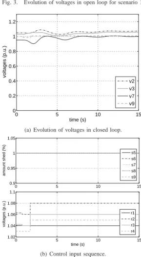
Fig. 4 depicts for scenario 1 the evolution of the system
when the proposed higher-layer MPC scheme is inserted in feedback. As shown the controller prevents the voltages from exceeding the upper and lower bounds by acting on the reference settings of all the AVRs. No load shedding is necessary. The system subsequently enters an acceptable steady-state condition with a constant input profile.
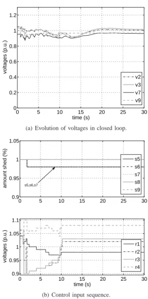
Fig. 6 depicts for scenario 2 the evolution of the system
with the MPC controller installed. Although the fault is significantly larger, the control prevents the voltages from crossing their limits, by providing set-points for the AVRs and shedding a minimal amount of load at node 7. After
about 20 seconds the system enters a new steady-state with
constant input profile. D. Discussion
The proposed controller works well for the studied cases, in which a rather high sampling rate of Ts = 0.25 seconds
was taken; indeed, this rate might have to be decreased in a more realistic setting, since the system is composed of large high-power components that may not allow for such a high actuation frequency. For the type of faults considered the simulations indicate that the predictions made with the linearized model are sufficiently accurate and that possible faults introduced due to saturation of the real system which are not modeled in the linearized system can be neglected. In fact, with a smaller fault, the sampling rate may be decreased, resulting in less frequent set-point updates to the
0 5 time (s) 10 15 0 0.2 0.4 voltages (p.u.) 0.6 0.8 1 1.2 v2 v3 v7 v9
Fig. 3. Evolution of voltages in open loop for scenario 1.
time (s) voltages (p.u.) 0 5 10 15 0 0.2 0.4 0.6 0.8 1 1.2 v2 v3 v7 v9
(a) Evolution of voltages in closed loop.
5 10 15 15 10 time (s) 5 0 1.02 1.04 1.06 1.08 1.1 voltages (p.u.) 0 0.9 0.95 amount shed (%) 1 1.05 r1 r2 r3 r4 s5 s6 s7 s8 s9
(b) Control input sequence.
Fig. 4. Simulation results for scenario 1 in closed-loop control with the proposed MPC supervisor.
lower control layer. With a smaller fault, the magnitude and frequency of oscillations occurring reduce in size.
VI. CONCLUSIONS AND FUTURE RESEARCH In this paper we have considered layered control of voltage instability in a particular power network. In this particular network a single higher-layer controller provides set-points to lower-layer controllers at discrete time steps such that the negative effects of voltage instabilities in the underlying physical system are minimized. The higher-layer controller
0 20 25 30 time (s) 15 10 5 0 0.2 0.4 0.6 0.8 1 1.2 voltages (p.u.) v9 v7 v3 v2
Fig. 5. Evolution of voltages in open loop for scenario 2.
time (s) 30 25 20 15 10 5 0 0 0.2 0.4 0.6 0.8 1 1.2 voltages (p.u.) v9 v7 v3 v2
(a) Evolution of voltages in closed loop.
0 5 time (s) 15 10 20 25 30 0.9 0.95 1 1.05 1.1 0.9 0.95 1 1.05 amount shed (%) voltages (p.u.) 0 5 10 15 20 25 30 s5,s6,s7 s9 s8 s7 s5 s6 r1 r2 r3 r4
(b) Control input sequence.
Fig. 6. Simulation results for scenario 2 in closed-loop control with the proposed MPC supervisor.
uses a model predictive control strategy to determine its actions. It uses a model based on a discrete-time linearized model of the continuous-time nonlinear dynamics given by a system of differential-algebraic equations (DAE). Simula-tions illustrate the potential of this supervisory approach.
Future research will focus on investigating the region of validity of the linearized model and if necessary replacing this with piecewise affine models; performing simulations on a network in which the neighboring loads and generators are not aggregated, whereas the supervisory controller uses an aggregated model; comparing the proposed approach with an approach that uses variable time steps to make the predictions, instead of the fixed time steps used currently; assessing the real-time technical viability of the method; and, investigating decentralized control schemes where the local controllers of several subnetworks negotiate among themselves on how they should determine their actions to obtain system-wide optimal performance.
ACKNOWLEDGMENTS
This research was supported by the project “HYbrid CONtrol: Taming Heterogeneity and Complexity of Networked Embedded Systems (HYCON)”, contract number FP6-IST-511368, the project “Multi-agent control of large-scale hybrid systems” (DWV.6188) of the Dutch Technology Foundation STW, an NWO Van Gogh grant (VGP79-99), and the BSIK project “Next Generation Infrastructures (NGI)”. We thank G. Hug-Glanzmann for her useful comments.
REFERENCES
[1] U.S.-Canada Power System Outage Task Force, “Final report on the August 14, 2003 blackout in the United States and Canada: causes and recommendations,” Tech. Rep., Apr. 2004. [Online]. Available: https://reports.energy.gov/BlackoutFinal-Web.pdf
[2] N. Jenkins, R. Allan, P. Crossley, D. Kirschen, and G. Strbac,
Embedded Generation. Padstow, UK: TJ International Ltd., 2000. [3] J. Bernussou and A. Titli, Interconnected Dynamical Systems:
Stabil-ity, Decomposition and Decentralisation. Amsterdam, The Nether-lands: North-Holland Publishing Company, 1982.
[4] R. G. Farmer and P. M. Anderson, Series Compensation of Power
Systems. Encinitas, California, USA: PBLSH, Inc., 1996.
[5] P. Kundur, Power System Stability and Control. New York: McGraw Hill, 1994.
[6] D. Karlsson and D. J. Hill, “Modelling and identification of nonlinear dynamic loads in power systems,” IEEE Transactions on Power
Systems, vol. 9, no. 1, pp. 157–163, Feb. 1994.
[7] T. V. Cutsem and C. Vournas, Voltage Stability of Electric Power
Systems. Dordrecht, The Netherlands: Kluwer Academic Publishers, 1998.
[8] J. M. Maciejowski, Predictive Control with Constraints. Harlow, UK: Prentice Hall, 2002.
[9] E. F. Camacho and C. Bordons, Model Predictive Control in the
Process Industry. Berlin, Germany: Springer-Verlag, 1995. [10] M. Morari and J. H. Lee, “Model predictive control: past, present and
future,” Computers and Chemical Engineering, vol. 23, pp. 667–682, 1999.
[11] L. R. Petzold, “A description of DASSL - A differential/algebraic system solver,” in 10th World Congress on System Simulation and
Scientific Computation, Montreal, Canada, Aug. 1983, pp. 430–432.
[12] K. E. Brenan, S. L. Campbell, and L. R. Petzold, Numerical Solution of
Initial-Value Problems in Differential-Algebraic Equations.
Philadel-phia, Pennsylvania, USA: SIAM, 1996.
[13] S. Leirens, J. Buisson, P. Bastard, and J.-L. Coullon, “A hybrid approach for voltage stability of power systems,” in Proceedings of
the 15th Power Systems Computation Conference, Li`ege, Belgium,
2005.
[14] T. Geyer, M. Larsson, and M. Morari, “Hybrid emergency voltage control in power systems,” in Proceedings of the European Control
Conference 2003, Cambridge, UK, Sept. 2003.
[15] A. Atamt¨urk and M. W. P. Savelsbergh, “Integer-programming soft-ware systems,” Annals of Operations Research, vol. 140, no. 1, pp. 67–124, Nov. 2005.
[16] J. Linderoth and T. Ralphs, “Noncommercial software for mixed-integer linear programming,” Optimization Online, Jan. 2005.