INDIVIDUAL LOSS RESERVING IN GENERAL INSURANCE USING NEURAL NETWORKS.
DISSERTATION PRESENTED
AS PARTIAL REQUIREMENT TO THE MASTERS IN MATHEMATICS
BY
ERNEST DANKWA
UNIVERSITÉ DU QUÉBEC À MONTRÉAL Service des bibliothèques
Avertissement
La diffusion de ce mémoire se fait dans le respect des droits de son auteur, qui a signé le formulaire Autorisation de reproduire et de diffuser un travail de recherche de cycles
supérieurs (SDU-522 – Rév.10-2015). Cette autorisation stipule que «conformément à
l’article 11 du Règlement no 8 des études de cycles supérieurs, [l’auteur] concède à l’Université du Québec à Montréal une licence non exclusive d’utilisation et de publication de la totalité ou d’une partie importante de [son] travail de recherche pour des fins pédagogiques et non commerciales. Plus précisément, [l’auteur] autorise l’Université du Québec à Montréal à reproduire, diffuser, prêter, distribuer ou vendre des copies de [son] travail de recherche à des fins non commerciales sur quelque support que ce soit, y compris l’Internet. Cette licence et cette autorisation n’entraînent pas une renonciation de [la] part [de l’auteur] à [ses] droits moraux ni à [ses] droits de propriété intellectuelle. Sauf entente contraire, [l’auteur] conserve la liberté de diffuser et de commercialiser ou non ce travail dont [il] possède un exemplaire.»
MODÉLISATION INDIVIDUELLE DES RÉSERVES EN ASSURANCE I.A.R.D. BASÉE SUR DES RÉSEAUX NEURONES.
MÉMOIRE PRÉSENTÉ
COMME EXIGENCE PARTIELLE DE LA MAÎTRISE EN MATHÉMATIQUES
PAR
ERNEST DANKWA
Tout d’abord, je voudrais remercier le Dieu Tout-Puissant pour sa grâce et ses bénédictions divines de vie et de soutien tout au long de ma période d’étude dans cette grande institution. Ensuite, ma profonde gratitude va à mon directeur de recherche, Mathieu Pigeon. Je le remercie pour tout son soutien, son inspiration, ses conseils et, surtout, son engagement envers l’excellence. Ils ont été essentiels non seulement pour le succès de ce travail mais aussi pour tout mon progrès et mon bien-être. Je suis également reconnaissant à tous les membres du corps professoral et au personnel du département de mathématiques qui ont créé un environnement d’étude productif pour moi . De plus, je reconnais la contribution significative de Co-operators qui a fourni les données sans lesquelles la rédaction de ce mémoire n’aurait pas été possible. Enfin, j’ai spécialement dédié ce travail à ma femme bien-aimée, Doris Borketey, à mes fils, Joshua et Mishael, à ma chère mère, Mary Ashyia, et à la mémoire de mon défunt père, S.M. Dankwa, en reconnaissance de leur amour et de leurs précieux sacrifices pour que mes études soient un succès.
LIST OF TABLES . . . v
LIST OF FIGURES . . . viii
RÉSUMÉ . . . x
ABSTRACT . . . xi
INTRODUCTION . . . 1
CHAPTER I GENERAL OVERVIEW . . . 3
1.1 The general insurance business . . . 3
1.2 Loss reserving and its importance in general insurance . . . 4
1.3 Legal requirements for loss reserves . . . 6
1.4 The claim development process . . . 8
1.5 Individual approach versus collective approach . . . 9
CHAPTER II CLASSICAL MODELS FOR LOSS RESERVING . . . 13
2.1 Literature review . . . 13
2.2 Loss triangles . . . 16
2.3 Chain-ladder method (CL) . . . 20
2.3.1 Mack’s model . . . 21
2.4 Generalized Linear Models (GLMs) . . . 25
2.4.1 Model selection and adequacy checks . . . 34
CHAPTER III INTRODUCTION OF STATISTICAL/MACHINE LEARN-ING TOOLS . . . 37
3.1 Literature review . . . 37
3.2 Neural networks . . . 39
3.2.1 Introduction . . . 39
3.2.3 Formal structure of the feed-forward neural networks . . . 42
3.2.4 Activation functions . . . 45
3.2.5 Estimation of parameters . . . 46
3.2.6 R packages for neural networks . . . 50
3.2.7 An illustrative example . . . 50
3.2.8 Strengths and weaknesses . . . 53
CHAPTER IV DESCRIPTION OF THE NEURAL NETWORK MODEL FOR LOSS RESERVING . . . 56
4.1 Background . . . 56
4.2 The individual framework for loss reserving . . . 57
4.3 Frequency-severity model . . . 58
4.3.1 Frequency model . . . 60
4.3.2 Severity model . . . 67
4.4 Predicting from the frequency-severity model . . . 69
CHAPTER V NUMERICAL ANALYSES . . . 72
5.1 Description and cleaning of data . . . 72
5.2 Descriptive statistics . . . 74
5.3 Application of classical models . . . 81
5.4 Application of new model . . . 83
5.4.1 Analyses of Frequency models . . . 83
5.4.2 Analyses of severity models and computation of RBNS reserves 87 5.4.3 Computation of RBNS reserves using classical generalized lin-ear models . . . 91
5.5 Comparison of results . . . 94
CONCLUSION . . . 105
APPENDIX A DATA DESCRIPTION AND SUMMARY STATISTICS . 107 APPENDIX B SUPPLEMENTARY RESULTS FOR CLASSICAL MOD-ELS . . . 116
APPENDIX C SUPPLEMENTARY RESULTS FOR NEURAL NETWORK MODEL . . . 119 C.1 Backpropagation method . . . 119 BIBLIOGRAPHY . . . 128
Table Page
2.1 A run-off loss triangle . . . 17
2.2 A data of loss payments made by an insurer . . . 18
2.3 Incremental Loss triangle . . . 19
2.4 Cumulative Loss triangle . . . 19
2.5 The complete cumulative Loss triangle . . . 24
2.6 Layout of Incremental Loss triangle under GLM . . . 30
2.7 Estimate of parameters of GLM Poisson using R package . . . 31
3.1 Incremental Loss triangle . . . 51
3.2 Training set of the fictitious data . . . 51
3.3 Estimated payments of the test set . . . 52
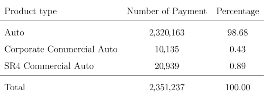
5.1 Distribution of payments by insurance product . . . 76
5.2 Incremental Loss triangle from the training set . . . 81
5.3 The summary of results for classical model . . . 83
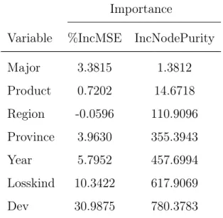
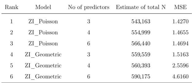
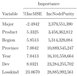
5.4 Results of random forest variable importance for number of payments 86 5.5 Results of the 1st six frequency models for the case when N is not categorized . . . 86
5.6 Results of the 1st six frequency models for the case when N is categorized . . . 87
5.7 Results of random forest variable importance for amount of payment 91 5.8 The summary of empirical results from neural network models with three predictors . . . 91
5.9 The summary of empirical results from neural network models with
five predictors . . . 92
5.10 The summary of empirical results from neural network models all seven predictors . . . 92
5.11 The summary of empirical results from GLM-Poisson models with three predictors . . . 93
5.12 The summary of empirical results from GLM-gamma models with three predictors . . . 93
5.13 Comparing empirical results of classical and neural network models 95 A.1 Description of variables in the training set . . . 108
A.2 Description of levels for the variable representing provinces . . . . 109
A.3 List of levels for the variable representing loss kinds . . . 110
A.4 List of levels for the variable representing valuation regions . . . . 111
A.5 Table showing payments made for each product type across all provinces . . . 112
A.6 Table showing payments made for each product type for all loss kinds . . . 113
A.7 Summary of payments by accident years . . . 114
A.8 Summary of payments by development years . . . 115
B.1 Further details of results of Mack model . . . 116
B.2 Further details of results of GLM-Poisson . . . 118
C.1 Results of the frequency models for the case when three predictors were used in the models . . . 121
C.2 Results of the frequency models for the case when four predictors were used in the models . . . 121
C.3 Results of the frequency models for the case when six predictors were used in the models . . . 122
C.4 The summary of empirical results from neural network models with four predictors . . . 122 C.5 The summary of empirical results from neural network models with
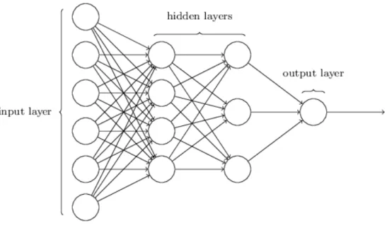
Figure Page 1.1 Claim development process. Adapted from (Duval & Pigeon, 2019). 8 3.1 A four-layer feed-forward neural network with two hidden layers
adapted from (Nielsen, 2015). . . 41
3.2 Plot of three most common activation functions used in neural net-works. . . 54
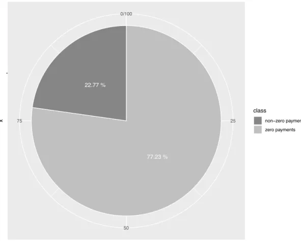
3.3 Estimated parameters of a two-layer feed-forward neural network. 55 5.1 Proportion of zero and non-zero payments made by the insurer . 75 5.2 Percentages of amount paid by provinces . . . 77
5.3 Proportions of total amount paid by development years . . . 78
5.4 Open and closed claims by accident years . . . 79
5.5 Chart showing frequency of reporting delay in years . . . 80
5.6 Trends of total payments in millions of dollars by accident and development years . . . 96
5.7 Predictive distribution of classical models . . . 97
5.8 Random forest variable importance plot for number of payment . 98 5.9 Random forest variable importance plot for amount of payment . 99 5.10 RBNS predictive distributions for neural network models with three predictors. . . 100
5.11 RBNS predictive distributions for neural network models with five predictors. . . 101
5.12 RBNS predictive distribution for neural network models with all seven predictors. . . 102
5.13 RBNS predictive distributions for GLM-Poisson severity models with three predictors. . . 103 5.14 RBNS predictive distributions for GLM-gamma severity models
with three predictors. . . 104 B.1 Supplementary plots from the Mack model . . . 117 C.1 RBNS predictive distributions for neural network models with four
predictors. . . 123 C.2 RBNS predictive distribution for neural network models with six
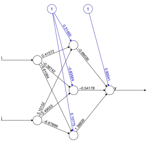
predictors. . . 125 C.3 Neural network plot of estimated parameters for three predictors. 126 C.4 Neural network plot of estimated parameters for five predictors. . 127
En assurance I.A.R.D, pratiquement tous les domaines d’activité tels que la con-ception de produits, la souscription, la tarification et la prise de décisions stratégi-ques et financières, peuvent être impactés par l’évaluation des réserves actuarielles. Les modèles classiques d’évaluation des réserves utilisent des données agrégées, souvent structurées sous la forme de triangles de développement. Dans de tels modèles, on suppose que les réclamations sont homogènes et que les paiements futurs ne dépendent que des années d’accident et de développement. Un incon-vénient majeur de ces modèles est de ne pas intégrer les caractéristiques individu-elles des réclamations qui peuvent permettre d’expliquer, en partie, l’hétérogénéité présente dans les données. Ces dernières années, cette hétérogénéité observée dans plusieurs bases de données d’assurance a motivé plusieurs chercheurs et chercheuses pour non seulement développer de nouvelles approches pour l’évalua-tion des réserves individuelles, mais aussi pour intégrer plusieurs outils d’apprentis-sage statistique afin de mieux prendre en compte les caractéristiques spécifiques des sinistres. Dans ce travail, nous explorons les réseaux de neurones en tant qu’outil d’apprentissage statistique et les intégrons dans un modèle d’évalua-tion individuelle des sinistres en assurance I.A.R.D. Nous proposons une approche de type fréquence-gravité dans laquelle un modèle linéaire généralisé est utilisé pour modéliser la fréquence des réclamations, et la sévérité des réclamations est mod-élisée à l’aide de réseaux de neurones. Nous appliquerons notre modèle à une base de données provenant d’une compagnie d’assurance canadienne et comparerons les estimations produites par ce modèle à celles obtenues à l’aide de certains modèles classiques.
Mots clés: Réserves individuelles, Réserve RBNS, Modèles linéaires généralisés, Modèle fréquence-sévérité, Apprentissage automatique, Réseaux de neurones.
In general insurance, virtually all areas of activity such as product design, un-derwriting, pricing, and strategic and financial decision making, can be impacted by the valuation of actuarial reserves. Traditional reserve valuation models use aggregate data, often structured in the form of development triangles. In such models, it is assumed that claims are homogeneous and that future payments depend only on years of accident and development. A major drawback of these models is that they do not integrate the individual characteristics of the claims which may help to explain, in part, the heterogeneity present in the data. In recent years, this heterogeneity observed in several insurance databases has mo-tivated several researchers to not only develop new approaches for the evaluation of individual reserves, but also to integrate several statistical learning tools in order to better take take into account the specific characteristics of claims. In this work, we explore neural networks as a statistical learning tool and integrate them into an individual claim assessment model in general insurance. We pro-pose a frequency-severity approach in which a generalized linear model is used to model the frequency of claims, and the severity of claims is modeled using neural networks. We will apply our model to a database from a Canadian insurance company and compare the estimates produced by this model with those obtained using some conventional models.
Keywords: Individual reserves, RBNS reserves, Generalized linear models, Fre-quency-severity model, Machine learning, Neural networks.
A unique feature of property and casualty insurance is that claims vary in several ways. While some claims may rarely occur, others may occur frequently. The amount of claims may also range from some few dollars to several billions of dollars. Moreover, while some claims may settle quickly, others may take several years to settle. For instance, following the September 11, 2001 terrorist attack in USA, Larry A. Silverstein, the leaseholder who suffered financial loss due to collapse of the building, claimed over $7 billion from his insurers. This led to a legal issue which was settled on December 2004 at an amount of $4.55 billion. Apart from the terrorist attack, the occurrence of floods and hurricanes have also had adverse impact on the insurance industry over the years. But irrespective of all these events, it is the primary responsibility of every insurer to ensure that an adequate amount of reserves is made available for the payment of future claims. However, for over several decades, the estimation and maintenance of loss reserves remain a major concern in property and casualty insurance. (Wenck, 1987) and (Leadbetter & Dibra, 2008) indicated that loss reserving is a major cause of insolvencies for several companies in the insurance industry.
This thesis explores a statistical/machine learning approach for loss reserving in the individual framework. It is not meant to be a comprehensive material on individual loss reserving and machine learning. However, it is laid out to give readers useful insights on existing loss reserving models and how the use of statis-tical/machine learning tools such as neural networks can help incorporate claim-specific features in loss reserving models. To an actuarial audience, it provides
significant contribution to the process of modeling and estimation of insurance data with respect to loss reserving. For a statistical audience, we make the con-cepts of statistical/machine learning more interesting by applying methods to real data set of an insurance company.
The rest of the work is organized as follows: In the first chapter, we will give a general overview of the property and casualty insurance to expose readers to the nature of the business and some concepts regarding loss reserving. In the second chapter, we shall discuss some classical models used for loss reserving and give an illustrative example. Next to that chapter, we shall discuss some statistical/machine learning tools and give theoretical and technical details of neural networks. We will introduce our proposed model for loss reserving in the fourth chapter, discuss the application of the classical and proposed models to an insurance data in the fifth chapter and draw conclusion of the studies.
GENERAL OVERVIEW
In this chapter, we shall expose our readers to property and casualty insurance business and highlight some key aspects of the business as well as some concepts regarding loss reserving.
1.1 The general insurance business
General insurance is a type of insurance that protects individuals and organiza-tions from the financial losses due to the occurrence of unpredictable events such as fire, motor accidents, flood, storm, earthquake, theft, travel mishaps and legal actions. In USA and Canada, general insurance is popularly known as property and casualty insurance while Europe and other parts of the world it is referred to as non-life insurance. By purchasing a general insurance policy, individuals and organizations, known as policyholders, transfer their financial risks to the insurance company, the insurer, in exchange for the payment of periodic (usually monthly or annual) amounts called premiums.
Some of the key operations insurers carry out in business include determining the right insurance products and features that meet their customers’ needs, select-ing and classifyselect-ing insured through a process called underwritselect-ing, usselect-ing analytic pricing methods to determine insurance cost and policy premiums, making
pay-ments for insurance claims and managing funds to ensure that adequate funds are made available to cater for future claims. The activities of insurance companies are regulated and governed by state laws. An insurer who fails to accumulate adequate resources for the payment of future claims becomes insolvent and may be required by law to cease operating. Therefore, in general insurance, the ability of an insurance company to meet its future obligations is very important to all stakeholders of the organisation including policyholders, management, investors and regulators.
1.2 Loss reserving and its importance in general insurance
The term loss reserve is described by Actuarial Standard of Practices (ASOP 43) as an insurer’s estimate of unpaid claims. It represents the insurer’s obligation for future payment resulting from claims due to the occurrence of events covered in the insurance policy. The term "technical provision" is also used in some actuarial literature to mean loss reserve. Loss reserve is usually the largest liability item for property and casualty insurers and it is a very significant factor used to determine the solvency of an insurance company. It is the responsibility of actuaries to develop, quantify, evaluate and monitor loss reserves.
Now, we shall examine the importance of accurate loss reserving practices to the key stakeholders of general insurance companies.
First and foremost, it is in the best interest of policyholders that reserves are estimated properly because they are direct beneficiaries of the payments of claims made by the insurance company. Insolvencies and defaults in the payment of claims adversely affect the standard of living of policyholders which cause the public and potential policyholders to lose faith in insurance as far as the provision of financial security is concerned. In order to prevent such misfortunes, insurers
must ensure they have adequate amount of money available to pay for future claims.
Unlike policyholders, investors are not direct beneficiaries of claim payouts, how-ever, they rely on the financial statements of insurance companies of which the estimate of loss reserves is a key input in most of the financial metrics. If reserves are miscalculated, the figures on balance sheets and income statements of the in-surer will be inaccurate. This means that the true financial position of the inin-surer will be misrepresented. Therefore, investors will not have accurate information to make effective decisions. Worst of it all, investors are likely to loss their in-vestment when an insurer becomes insolvent. Therefore, investors have interest in accurate loss reserving and good solvency measures of insurers.
Apart form policyholders and investors, the managers in the various department of an insurance company also, directly or indirectly, depend on accurate loss re-serving in order to make effective decisions on company operations such as product development, pricing, underwriting, strategic and financial decisions.
Accurate loss reserving helps the product development department to determine appropriate features of insurance products such as limits and deductibles of in-surance as well as reinin-surance needs for an inin-surance product. Estimates of loss reserves also affect pricing of insurance products. Underestimation of reserves can influence the insurer an insurer to lower premium of insurance products. This can lead to inability to pay for future claims. On the other hand, overestimation of reserves can influence the insurer to increase premium of insurance products. In that case, the insurer may loss its market share to another insurer offering com-petitive products at more affordable premiums. The claim department also need accurate loss reserving so that adequate amount will be available to carry out their functions such as payment of claims and legal costs. Accurate loss reserving
is also necessary for managers to make financial and strategic decisions such as investment of funds, allocation of capital among lines of business, entry and exit of lines business.
From the fiscal point of view, improper estimates of loss reserves has impact on the amount of taxes the insurance company pays to the government. Overesti-mation of loss reserves reduces the company’s taxable income for the company to pay less taxes to the government. However, the practice of using high level of loss reserve as a tax evasion mechanism is not encouraged since the company may end up having issues with tax authorities. In addition to that, announcements of high reserves may have adverse effects on share values, bond rating and man-agerial compensations because shareholders and bondholders may have difficulty distinguishing tax-motivated reserve from those that reflect true economic risks of the company.
Last but not least, insurance regulators rely on the financial statements of an insurer to carry out their supervisory role. Inaccurate reserves could result in a misstatement of the true financial position of an insurer. According to (Friedland, 2010), if a financially struggling insurer masks its true state with inadequate re-serves, a regulator may not become involved to help the insurer regain its strength until it is too late.
1.3 Legal requirements for loss reserves
Apart from protecting the interests of all stakeholders, it is important to mention that proper estimation of unpaid claims by insurers is a legal requirement. For instance, (Friedland, 2010) stated a New York insurance law passed in the early 1960s which says that "... every insurer shall maintain reserves in an amount estimated in the aggregate to provide for the payment of all losses or claims
incurred on or prior to the date of settlement whether reported or unreported which are unpaid as of such date and for which such insurer may be liable, and also reserves an amount estimated to provide for the expenses of adjustment or settlement of such claims." These days, the role of the Appointed Actuary has been created through insurance legislation in countries around the world to meet the legal requirements for accurate estimation of unpaid claims.
In Canada, the Insurance Companies Act (1991) stipulates federal laws that gov-ern the insurance industry. In this Act, the Office of the Superintendent of Fi-nancial Institutions (OSFI) is mandated to be the primary regulator of insurance companies responsible for setting guidelines concerning capital and solvency of insurers as well as standards for financial reporting. The Insurance Companies Act requires all federally regulated insurers to have an appointed actuary. It is a legal responsibility of the appointed actuary to value the actuarial and other policy liabilities of the company at the end of a financial year.
International Accounting Standards Board (IASB), an independent international organization for accounting and financial reporting, in the year 2005, issued Inter-national Financial Reporting Standard (IFRS 4) as the first guidance on account-ing for insurance contracts. The standard requires the disclosure of information that will help users understand the amounts in the insurer’s financial statements and evaluate the nature and extent of risks arising from insurance contracts. As of 1 January 2021, the IFRS 4 will be replaced by IFRS 17 which has more detailed approach to measurement and disclosure of an insurer’s obligations from insurance contracts irrespective of the nature of the contracts. OSFI formally recognized the IFRS 17 in May 2018, hence placing emphasis on maintaining capital requirement and solvency of insurers as well as creating comparable financial reporting across international boundaries.
1.4 The claim development process
In general insurance, the final settlement of claims usually takes some time. Every claim goes through a process before it is finally settled. The development process for a claim with number, say k, can be illustrated by a timeline as shown Figure 1.1. The occurrence/accident date is the exact date which the event that caused
Figure 1.1 Claim development process. Adapted from (Duval & Pigeon, 2019).
the financial loss occurred while the reporting date is the date on which the insured informed the insurer of the occurrence of the accident. It is common that the date of the accident may not be the same as the reporting date and the insurer may not be aware of the existence of a claim until several years later. When the occurrence of the accident is not reported to the insurer on the same date as the accident date, the time-lag between the accident date and the reporting date is called reporting delay. In Figure 1.1, for instance, T1(k) and T2(k) represent occurrence and reporting dates, respectively, and the time between T1(k) and T2(k) represents reporting delay. This situation is more frequent for liability insurance claims. Between the accident date and reporting date, the claim is said to be Incurred But Not Reported (IBNR).
After the accident is reported the settlement of the claim may take several years due to legal activities. Until a claim finally settles on a closing/settlement date, the insurer may make an initial payment and several other payments (or refunds).
In Figure 1.1, for instance, the final settlement occurred at T3(k). Before that date, M payments, Pt(k)
1 ,Pt(k)2 , . . . ,Pt(k)M were made at times t (k)
1 ,t2(k), . . . ,tM(k), respectively. Whereas claims from property insurance usually settle faster, claims from liability insurance or bodily injury often take a long time to settle. The time-lag between the reporting date and the settlement date is called closing/settlement delay. From Figure 1.1, the time between T2(k) and T3(k) represents closing/settlement delay. During the period between the reporting date and settlement date, the claim is said to be Reported But Not Settled (RBNS). Even after the settlement of a claim, the closed claim can be reopened due to unexpected new development or if a relapse occurs (Wüthrich & Merz, 2008). This will also call for several other payments before the claim finally closes.
When insurance companies do their periodic evaluations, it is expected by law that they estimate the total of unpaid claims. Actuaries, the professionals mandated to estimate reserves, put together Reported But Not Settled (RBNS) claims and Incurred But Not Reported (IBNR) claims to arrive at the total of unpaid claims.
1.5 Individual approach versus collective approach
Based on the granularity of data used to estimate loss reserves, a loss reserving model can be classified as a collective approach or an individual approach. In a collective approach for loss reserving, aggregate data for an entire portfolio is used for loss reserving. Usually, in a collective approach, individual claims are aggregated by accident period and developing delays and organized in a run-off loss triangle. (Denuit & Trufin, 2018) used a collective approach of loss reserving for long-tailed claims data. Classical models such as the chain-ladder and Mack’s model are based on the collective approach.
• They are easy to understand since the loss data is summarized in a run-off triangle.
• They are easy to implement since they apply straightforward formula. • They can be used with minimum computational requirements.
Despite the above advantages, the collective loss reserving models have the fol-lowing disadvantages.
• Collective models undermine heterogeneity in claims by their inability to incorporate any information about the individual claims.
• The pattern of claims do not remain the same for the future as it is assumed in some collective models such as the chain-ladder (Friedland, 2010). • According to (England & Verrall, 2002), the observed data in a run-off
triangles is typically small leading to large prediction error.
• (Charpentier & Pigeon, 2016) pointed out that the results of aggregate mod-els will not be enough when modern solvency laws call for full conditional distribution of future cash flows.
• With collective models there is a misalignment of risk functions when ratemak-ing is based on individual data and reservratemak-ing is based on aggregate data. • Some collective models such as the chain-ladder model only give best
esti-mates of reserve without providing any information about the variability of reserve and the level of risk.
On the other hand, the individual approach of loss reserving models the loss reserves of claims on individual policies. The total reserve is the sum of all reserves
of the various policies in the portfolio. The individual approach facilitates the study of each single claim to know its ultimate amount. One can also include claim specific features in the estimation of reserves. (Huang et al., 2015) and (Pigeon et al., 2013) presented examples of individual approach for loss reserving. Advantages of individual loss reserving models include the following.
• Unlike collective loss reserving models, the individual loss reserving models allow claim specific information to be incorporated in the loss reserving models.
• They offer much simpler way to investigate frequency and severity of claims separately.
• Individual loss reserving models provide information about variability of reserve.
• They help to align loss reserving with ratemaking function which is mostly based on individual data.
• They relax the assumption that the pattern of claim remain the same for future.
• They enable the establishment of reserves that meet modern solvency re-quirements. Risk of the insurer can be determined from full conditional distribution of future losses.
Despite the above advantages, the individual loss reserving models have the fol-lowing disadvantages.
• They are data oriented and require huge data to make meaningful predic-tions of future losses.
• The size of individual loss data tends to be huge which mean they require high computing powers.
• Individual loss reserving models tend to be more complicated than the col-lective loss reserving models.
After considering the individual and collective approaches to loss reserving, we decide to adopt the individual loss reserving approach in this work for two main reasons:
1. The advantages of the individual loss reserving approach far exceed that of the collective loss reserving approach.
2. Current solvency laws stipulated by the Office of the Superintendent of Fi-nancial Institutions (OSFI) require insurers to establish reserves that reflect the true risk of the company. Individual loss reserving approach ensures the compliance of modern solvency laws.
Therefore, we shall point it out that this research will give more attention to individual loss reserving methods. Readers interested in more applications of collective models should see (Wüthrich & Merz, 2008).
CLASSICAL MODELS FOR LOSS RESERVING
Loss reserving methodology has developed from very simple models to modern day complex ones. In this chapter, we shall discuss some classical models used for loss reserving in general insurance such as the chain-ladder (CL), Mack’s model (MC) and generalized linear models (GLMs).
2.1 Literature review
Over the past 30 years, various researchers have made significant contributions towards the development of models for loss reserving in general insurance. While some of these models are stochastic, others are deterministic. A useful taxonomy of loss reserving models over the years can be found in (Taylor, 2000). In general, there have been increased interest in stochastic claim reserving in recent times. That is, there is a substantial growth in loss reserving models that are defined in probabilistic environments to induce randomness in output rather than models whose output are fully determined by parameter values. However, the stochastic models are only used by a limited number of practitioners (England & Verrall, 2002). The deterministic models were first developed as computational algorithms that focused mainly on obtaining estimates for reserves. Although the stochastic models are less dominant in current loss reserving practices, various researchers
have used them to extend the assumptions of the deterministic models so that uncertainties of reserve estimates and even full predictive distributions of reserve estimates can be provided along with reserves estimates. Overview of the deter-ministic and stochastic models can be found in (Taylor, 2000), (England & Verrall, 2002), (Wüthrich & Merz, 2008) and (Friedland, 2010).
In loss reserving for general insurance, it is well known that the most fundamental method underlying both deterministic and stochastic methods is the chain-ladder. The basic idea of this method was already known to (Tarbell, 1934). The chain-ladder method is a deterministic approach to loss reserving traditionally based on run-off triangles. However, the stochastic version of the chain-ladder which allows the estimation of mean square error of estimated reserves can be found in (Mack, 1993) and (Mack, 1999).
In recent years, several researchers have contributed to various extensions of the chain-ladder model. For instance, (Gogol, 1993) and (Verrall, 2004b) proposed models that combine prior information derived from expert opinion on total cost of claims or estimate of loss ratio with observations from a database. (Miranda et al., 2012) also proposed a double chain-ladder model that make use of triangles developed from paid and incurred losses.
The chain-ladder method calculates loss reserves using run-off triangles of paid and incurred losses representing the sum of paid losses and case reserves. The approach is considered to be a collective or macro-level loss reserving (Wüthrich & Merz, 2008). In essence, the method works under the assumption that patterns of claims activities in the past will continue to be seen in the future (Friedland, 2010).
The limitations of the chain-ladder method and other macro-level reserving mod-els have been discussed by some researchers. These limitations include
over-parametrization of the chain-ladder method ((Wright, 1990) and (Renshaw, 1994)); unstable predictions for recent accident years (Bornhuetter & Ferguson, 1972); problems with the presence of zero or negative cells in run-off triangles (Kunkler, 2004); difficulties in separate assessment of RBNS and IBNR claims ((Schnieper, 1991) and (Liu & Verrall, 2009)) and difficulties in the simultaneous use of in-curred and paid claims (Quarg & Mack, 2004).
Various contributions have been made by researchers to address the issues of the chain-ladder method. (Bornhuetter & Ferguson, 1972) built a loss reserving model that incorporates prior information about the insurers exposure to loss. (Verrall, 2004a) and (Meyers, 2007) advanced the traditional loss reserving methods by combining the chain-ladder and Bornhuetter-Furguson methods with Bayesian methodology. This enabled them to derive predictive distributions for future losses. Other researchers developed methods to obtain variability of estimates and mean square error of prediction. For instance, (Schnieper, 1991) and (Liu & Verrall, 2009) suggested using simulations based on separate RBNS and IBNR run-off triangles.
Some researchers viewed the problem of loss reserving from the perspective of regression models. (Halliwell, 1996) introduced a generalized least-squares ap-proach in loss reserving. Further contributions to this apap-proach were made by other authors including (Hamer, 1999) and (Ludwig et al., 2011).
Since the early 1990s, the use of generalized linear regression in loss reserving has gained increasing interest in actuarial literature. There exist an extensive literature that investigate the statistical basis of the chain-ladder method with a focus on the distributional assumptions of the aggregate data and the use of generalized linear regression models. For example, (Murphy, 1994) and (Bar-nett & Zehnwirth, 2000) studied the chain-ladder technique within the context
of normal linear regression. (England & Verrall, 2002) revealed that a normal model as an approximation to the negative binomial model provides a link to Mack’s model. (Wright, 1990) and (Mack, 1991) also studied the link between the chain-ladder technique and the Poisson distribution. The implementation of the Poisson distribution using standard statistical methodology can be found in (Renshaw & Verrall, 1998). (Verrall, 2000) provided more details on the negative binomial model and its relationship to the over-dispersed Poisson model. The gamma model proposed by (Mack, 1991) also received considerable attention in literature. (Wüthrich, 2003) generalised the gamma cell distribution model in (Taylor, 2000) by using the Tweedie’s compound Poisson distribution for claims reserving.
Having reviewed the some of the work done in literature, we shall describe the chain-ladder, Mack’s model and generalized linear models in details.
2.2 Loss triangles
Estimates for macro-level models are often based on run-off triangles that summa-rize loss data based on occurrence/accident years and development years. Table 2.1 gives the format of a loss triangle over I and J accident and development years, respectively. For accident years i, i = 1, . . ., I, and development years j, j = 1, . . . , J, Ci, j represents the cumulative amount of payment for the loss. An incremental loss triangle can be obtained from the cumulative loss triangle by taking the difference of cumulative payments for successive development years. That is,
Yi,1 = Ci,1, i = 1, . . . , I
Table 2.1 A run-off loss triangle Development year Acc. year 1 2 3 . . . J 1 J 1 C1,1 C1,2 C1,3 . . . C1,(J 1) C1,J 2 C2,1 C2,2 C2,3 . . . C2,(J 1) .. . ... ... ... . . .
i Ci,1 Ci,2 . . . Ci,(J i+1) ..
. ... ... . . .
I CI,1
Yi, j is described as incremental payment for accident year i and development year j. The cumulative loss triangle forms the basis of the macro-level models discussed in the subsequent sections.
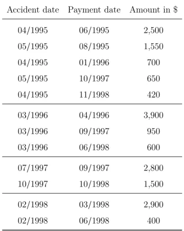
We shall use Table 2.2 as a fictitious loss data of an insurer to illustrate the concepts in classical loss reserving.
Example 2.2.1. The information provided in the records of the insurer can be explained as follows: In the year 1995, two accidents occurred in April and May, respectively. For those accidents, five payments have been made by the insurer from the year 1995 through to 1998. In the year 1996, one accident occurred of which 3 payments have been made as of year 1998. Two accidents occurred in the year 1997 and two payments have been made as of year 1998. Finally in the year 1998, one accident occurred of which two payment have been made by the insurer.
In Example 2.2.1, an incremental loss triangle can be construct by taking note of the following
Table 2.2 A data of loss payments made by an insurer Accident date Payment date Amount in $
04/1995 06/1995 2,500 05/1995 08/1995 1,550 04/1995 01/1996 700 05/1995 10/1997 650 04/1995 11/1998 420 03/1996 04/1996 3,900 03/1996 09/1997 950 03/1996 06/1998 600 07/1997 09/1997 2,800 10/1997 10/1998 1,500 02/1998 03/1998 2,900 02/1998 06/1998 400
following the notation in Table 2.2, we have: i = 1, . . ., 4, which corresponds to the years 1995, 1996, 1997 and 1998, respectively.
• We have four development years since the records indicate payments were made for losses in the years from 1995 through to 1998. Also, following the notation in Table 2.2, we have j = 1, 2, 3, 4.
The incremental loss triangle summarizes the total amount of loss paid in the development years, j, for each accident, i. For instance, in accident year 1995, a total payment of 4,050 (i.e. 2,500+1,550) was made in the development year 1; 700 was made in development year 2; 650 was made in development year 3; and 420 was made in development year 4 etc. The summary of incremental losses for
Example 2.2.1 is given in Table 2.3.
Table 2.3 Incremental Loss triangle Development year Acc. year 1 2 3 4 1995 4,050 700 650 420 1996 3,900 950 600 1997 2,800 1,500 1998 3,200
The cumulative loss triangle sums all loss made up to a development years, j, for each accident, i. For instance, in accident year 1995, a total payment of 4,050 (i.e. 2,500+1,550) was made in the development year 1; 4,750 (i.e. 4,050+700) was paid in development year 2; 5,400 (i.e. 4,750+650) was paid in development year 3; and 5,820 (i.e. 5,400+420) was paid in development year 4 etc. The summary of cumulative losses for Example 2.2.1 is given in Table 2.4.
Table 2.4 Cumulative Loss triangle Development year Acc. year 1 2 3 4 1995 4,050 4,750 5,400 5,820 1996 3,900 4,850 5,450 1997 2,800 4,300 1998 3,200
2.3 Chain-ladder method (CL)
Among all the loss reserving techniques, the chain-ladder method is the most popular, both in theory and practice. The method is recognized in actuarial lit-erature as a computational algorithm for the estimation of loss reserves. (Mack, 1993) presented a distribution-free derivation of the chain-ladder method. Several extensions of the technique have been made in literature including conditional pre-diction error of the distribution free CL method and multivariate CL (Wüthrich & Merz, 2008). As proposed by (Mack, 1993), the key assumptions of the distri-bution free chain-ladder are defined as follows:
Definition 2.3.0.1 (Chain-ladder method).
(CL1): Cumulative claim amounts for different years of occurrence are independent. (CL2): There exist development factors j such that Ci,(j+1) = jCi, j, for i = 1, . . ., I
and j = 1, . . ., J 1.
The development factors of the CL method, j, are unknown and estimated by the expression below:
bj = ÕJ j i=1 Ci,(j+1) ÕJ j i=1 Ci, j for j = 1, . . ., J 1.
Furthermore, the estimator for the total cost of claims for each year of occurrence and that of reserve as given as follows:
b
Ci,J = (bJ i+1⇥ . . . ⇥ bJ 1)Ci,(J i+1) b
Ri = Cbi,J Ci,(J i+1) b R = I ’ i=2 b Ri.
The algorithm functions under the assumption that the pattern of claim activities in the past will be the same for future claims. It is shown that the development factors are uncorrelated even though they are not independent. Another useful property under the assumptions given above is that the estimator of the total claim is unbiased hence providing a justification for the reserve estimates. These properties and other related ones are well illustrated in (Wüthrich & Merz, 2008). Despite the fact that the method is intuitive and simple, it has several flaws:
• The development factor is identical for all years of occurrence which is not the case in practice if there is a change in jurisdiction or management. • It is impossible to make an estimate of the accuracy of estimate since the
method is deterministic. Confidence intervals of estimated reserves cannot be easily obtained using the algorithm.
• Individual claim characteristics are not incorporated in the algorithm. • Over-parametrization may affect recent estimates of reserve since the
eval-uation of reserve tends to be a product of many estimates.
2.3.1 Mack’s model
The stochastic version of the CL algorithm was proposed by Mack (1993). The advantage of Mack’s model is that, the model enables one to estimate the uncer-tainties of the reserve estimates in addition to estimates for reserves. The Mack’s model has interesting properties and has laid the foundation for many research works in loss reserving.
In the Mack’s model, the cumulative amount of claims payment for accident year, i, and development year, j, is denoted by Ci, j, for i = 1, . . ., I and j = 1, . . ., J.
Given below are the hypothesis of the Mack model: Definition 2.3.1.1 (Mack’s model).
(MC1): Cumulative claim amounts for different years of occurrence are independent. (MC2): The development factors, 1, . . . , J 1 and cumulative payments satisfy the
expression below:
E[Ci,(j+1)|Ci,1, . . . ,Ci, j] = jCi, j for j = 1, . . ., J 1.
(MC2b): The cumulative payments, (Ci, j), j = 1, 2, . . . form a Markov chain and there exist strictly positive variance parameters, 2
1, . . . , J 12 , such that for 1 i J and 1 j J 1, we have the expression below:
Var[Ci,(j+1)|Ci,1, . . . ,Ci, j] = 2jCi, j.
Similar to the chain-ladder algorithm, the development factors are estimated by bj = ÕJ j i=1 Ci,(j+1) ÕJ j i=1 Ci, j for j = 1, . . ., J 1.
The variance parameters are also estimated as follows: b2 j = J 1j 1 J j ’ i=1 Ci, j⇣Ci,(j+1)C i, j bj ⌘2 b2 J 1 = min hb4 J 2 b2 J 3 ,min⇣bJ 32 ,bJ 22 ⌘i.
The hypotheses bring out very useful properties of the Mack’s model some of which are given as follows:
• Concerning ultimate cost of claims we have
E[Ci,J|Ci,(j i+1)] = Ci,(j i+1) J 1 J 2. . . j i+1, for 1 i J. • The estimator, bj is an unbiased estimator for j.
• The estimators b1, . . . , bJ 1 are uncorrelated.
• Given Ci,(j i+1), bCi,J is an unbiased estimator for E[Ci,J|Ci,(j i+1)]. • bCi,J is an unbiased estimator for E[Ci,J].
• The estimator, b2j, is an unbiased estimator for j2.
Details about the estimators of the Mack’s model, proof of the their properties and other useful remarks can be found in (Wüthrich & Merz, 2008).
Using the Mack’s model, the estimate for reserve for accident year, i, is given by E[Ci,J|Ci,(j i+1)] Ci,(j i+1) =Ci,(j i+1)(bj i+1⇥ . . . ⇥ bJ 1 1).
Consequently, the reserve estimate for the Mack’s model and that of the chain-ladder algorithm are the same.
Example 2.3.1. In this example, we recall Table 2.4 which is the cumulative loss triangle for Example 2.2.1. We shall give an illustration of how the development factors and reserves are estimated. The result is the same for both the Mack’s model and the chain-ladder method.
By applying the expression of the estimator given in sections 2.2 and 2.3, we can calculate the development factors as:
b1 = 4,750+4,850+4,3004,050+3,900+2,800 = 1.293023 b2 =
5,400+5,450
4,750+4,850 =1.130208 b3 = 5,8205,400 = 1.077778.
amount as follows; b C2,4 = C2,3⇥ b3 =5,450 ⇥ 1.077778 = 5,873.889 b C3,3 = C3,2⇥ b2 =4,300 ⇥ 1.130208 = 4,859.896 b C3,4 = C3,2⇥ b2⇥ b3= 4,300 ⇥ 1.130208 ⇥ 1.077778 = 5,237.888 b C4,2 = C4,2⇥ b3 =4,137.674 b C4,3 = C4,3⇥ b1⇥ b2= 4,676.434 b C4,4 = C4,4⇥ b1⇥ b2⇥ b3 =5,040.157.
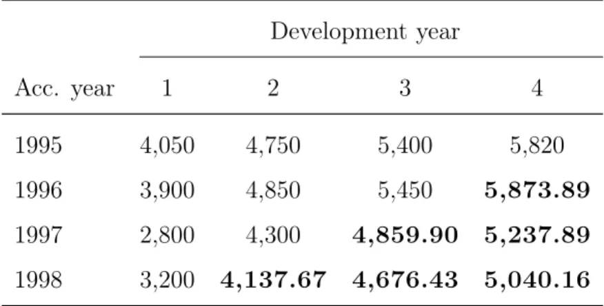
The above results helps to complete Table 2.4 by filling the unknown values in the lower portion of the table. The complete table of known loss amounts and the predicted loss amounts (in bold characters) for the insurer is shown in Table 2.5.
Table 2.5 The complete cumulative Loss triangle Development year Acc. year 1 2 3 4 1995 4,050 4,750 5,400 5,820 1996 3,900 4,850 5,450 5,873.89 1997 2,800 4,300 4,859.90 5,237.89 1998 3,200 4,137.67 4,676.43 5,040.16
Once the table is completed, we apply the formulas for estimating reserves, bRi. That is, the values on the diagonal, representing the latest loss amounts, are sub-tracted from the corresponding ultimate loss (found on the last column of the table) to get the reserves for each accident year. The total reserve is the sum of all the
calculated accident year reserves. This is illustrated below: b R2 = Cb2,4 C2,3 =5,873.89 5,450 = 423.89 b R3 = Cb3,4 C3,2 =5,237.89 4,300 = 937.89 b R4 = Cb4,4 C4,1 =5,040.16 3,200 = 1,840.157 b R = 4 ’ i=2 b Ri = 3,201.93.
Even though the Mack’s model for loss reserving is widely applied, easy to under-stand and produces a measure of uncertainty unlike the traditional chain ladder, it has some drawbacks that have drawn the attention of several authors. For example:
• Over-parametrization issue can lead to loss of predictive power since a lot of information that are not included in the estimation of the parameters become useless ((Wright, 1990).
• Non-robustness to outliers and failure of the method to include tail factors (Verdonck et al., 2009).
• Unstable prediction for recent accident years (Bornhuetter & Ferguson, 1972).
2.4 Generalized Linear Models (GLMs)
The use of Generalized linear models in loss reserving is described as parametric methods that allow assumptions to be made on the distribution of claim amounts. Generalized linear models (Nelder & Wedderburn, 1972) were developed as a generalization of the ordinary linear regression. In general, when we have a data
of size n and p set of covariates, the ordinary linear regression model can be written mathematically as:
Yi = 0+ 1Xi1+ 2Xi2+ . . . + pXip+ "i, i = 1, ..., n
where: Yi and Xi1, . . . ,Xip represent the ith observation of the response and pre-dictor variables, respectively; 0. . . p are regression parameters, and "i is the ith residual value which is assumed to be independent and normally distributed with mean 0 and constant variance, 2.
Linear regression models are easy to understand and implement. Results are also easy to interpret. However, for practical purposes, there are several drawbacks:
• The normality assumption is very restrictive. Most insurance data do not follow normal distribution.
• The constant variance assumption does not hold in real application.
• Application of a normal model is affected by issues with real data sets such as missing values, collinearity, high percentage of zeros etc.
The introduction of Generalized linear models relaxes the normality assumption imposed by the ordinary linear regression and allows the response to come from a large family of distributions called the linear exponential family which includes the normal distribution. The probability density function of random variable, Y, whose distribution is a member of the linear exponential family, is given by:
fY(y; ✓, ) = c(y; )exp
⇣y✓ a(✓)⌘ ,
where ✓ is referred to as canonical parameter; , a dispersion parameter, a(·), a log-partition function and c(·), a base function.
Members of the linear exponential family such Bernoulli, Binomial, Poisson, gamma, normal, and inverse-gaussian distributions have desirable statistical properties. For instance, the mean and variance of the response variable can be specified, respectively, as;
E[Y] = a0(✓) = µ Var[Y] = a00(✓).
Generalized linear models allow for the choice of a link function, g, whose inverse transforms the linear predictor to get the target response variable. That is, an appropriate link function, not necessarily linear, can be chosen under GLM ap-proach to expresses a relationship between the linear predictor and the mean of the response. Thus, we have,
g(E[Yi]) = g(a0(✓i)) = X0i . In other words:
E[Yi] = g 1(X0i ), where represents regression parameters and X0
irepresents a vector of explanatory variables for the ith observation. Therefore, the mean of the response vary with the characteristics of the individual observations. This implies that, unlike the classical linear regression, the variance of the response under GLM, is not constant but a function of the mean which may vary with regressors.
The estimation of parameters under GLM follow maximum likelihood procedures. The log-likelihood function is given by:
l(y; , ) = n ’ i=1 ln⇣f (yi, , ) ⌘ = n ’ i=1 ln⇣c(yi, ) ⌘ + ⇣yi✓ a(✓)⌘.
When the first derivative of the log-likelihood, l(y; , ) is taken with respect to the parameters and set to zero, we arrive at the system of estimating equations given by: @l(y; , ) @ t = n ’ i=1 yi µi g0(µi)a00(✓i)xi,t =0, t = 0, 1, . . . , p.
Usually, it is not convenient to solve the equations by hand. They are solved using numerical methods. The inverse of the Fisher information matrix gives the variance of the parameters as follows:
Var[b] = I(b) 1= n ’ i=1 1 g(µi)2Var[Y i]2xi,txi,u,
where t = 0, 1, . . ., p and u = 0, 1, . . ., p. It has been shown that, by the law of large numbers, the estimator for asymptotically follows a normal distribution with mean zero and variance equal to the inverse of the fisher information matrix. That is:
p
n(b ) ! N(0, I 1( )), as n ! 1.
GLM is used as a collective approach for loss reserving by making a distribution assumption on the incremental loss payments, Yi, j. For instance, it is popular to assume that Yi, j follows a Poisson distribution which is a member of the linear exponential family. As seen in the previous classical models, the accident years, i, and development year, j, are used as predictor variables to explain the response variable, Yi, j under the hypothesis below:
Definition 2.4.0.1(Generalized Linear Model for increments).
(GLM1): The random variable Yi, j for different accident years and/or development years are independent.
(GLM2): The probability density function of random variable Yi, j ,is f (y; ✓i, j, i, j) = c(y; i, j)exp⇣ y✓i, j a(✓i, j)
i, j ⌘
,
where ✓ is referred to as canonical parameter; , a dispersion parameter, a(·), a log-partition function and c(·), a base function.
We summarize the structure of the stochastic models for claim reserving in the framework of generalized linear models as follows:
• The incremental claim amounts Yi, j belongs to the exponential family. • E[Yi, j] = µi, j is the mean function.
• ⌘i, j = g(µi, j), where g(·) is the link function.
• The linear predictor ⌘i, j, is a linear combination of factor effects i and j.
We consider a multiplicative structure with parameter for each row, i, and each column j as given below:
E[Yi j] = ↵i⇥ j.
Here, the factor effect, ↵i, denote expected exposure of the accident year while j denote expected cashflow of the development year. The multiplicative structure is linearized naturally by the choice of a logarithmic link function. With the logarithm link given as g(·) = ln(·). Therefore,
⌘i, j = ln(E[Yi, j]) = ln(↵i) + ln( j).
The model can be made identifiable by imposing additional constraints such as Õ
j j = 1and ↵1 =1. Then we have 2J 1 parameters to estimate given by:
A regression problem comes out when we define a the design matrix for the linear predictor.
Z1,j = [0 . . . 0 0 0 0 . . . 0 1 . . .]0 Zi, j = [0 . . . 1 0 0 0 . . . 0 1 . . .]0,
where the 1’s correspond to positions where i and j are observed respectively. Thus, we can write the mean in a convenient form as follows:
E[Yi j] = eZi, j .
The estimates for the parameters are obtained using maximum likelihood proce-dures. Then, the estimates of future increment payments is given by
bYi, j = g 1(b0+b↵i+bj).
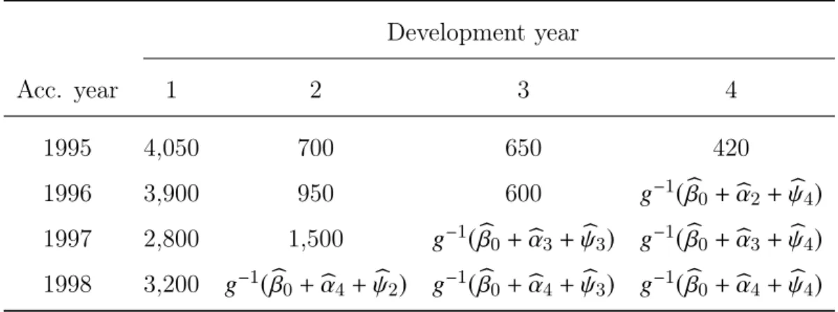
Example 2.4.1. With reference to the increment table in Example 2.2.1, the GLM layout will be of the form in Table 2.7.
Table 2.6 Layout of Incremental Loss triangle under GLM Development year Acc. year 1 2 3 4 1995 4,050 700 650 420 1996 3,900 950 600 g 1(b0+b↵2+ b 4) 1997 2,800 1,500 g 1(b0+b↵3+b3) g 1(b0+b↵3+ b4) 1998 3,200 g 1(b 0+b↵4+ b2) g 1(b0+b↵4+b3) g 1(b0+b↵4+ b4)
We estimate the unknown parameters ↵i and j from the triangle of known data with the maximum likelihood method. The estimate of reserve is the sum of
predicted claims for the unknown part of the triangle. In the following, we use the notation 5 for the lower triangle of data, i.e., the set of all (i, j), where Yi, j is unknown but predicted using the GLM parameter estimates. Then,
ˆ R = ’
i, j25 bYi, j.
Example 2.4.2. In this example we illustrate how to obtain the parameters of a GLM for the data given in Example 2.2.1. First, we assume that the increments follow a Poisson distribution which is a member of the linear exponential family. With a multiplicative structure for the row effects and column effects, a natural choice of link function the logarithmic function. Using R package, we implement the GLM estimation by specifying a data frame which consist of the increment payments and their corresponding accident years, i, and development years, j. The results of estimated parameters from the R package are given in Table 2.8.
Table 2.7 Estimate of parameters of GLM Poisson using R package Parameter Estimate Intercept: b0 8.214769 b↵2 0.009217 b↵3 -0.105382 b↵4 -0.143863 b2 -1.227503 b3 -1.781636 b4 -2.174514
The estimated parameter are used to predict the unknown incremental values fol-lowing the structure in Table 2.7. The sum of the predicted values gives the
esti-mate of reserves. bY2,4 = exp(b0+b↵2+ b4) = exp(8.21477 + 0.00922 + 2.17451) = 423.8889 bY3,3 = exp(b0+b↵3+ b3) = exp(8.21477 + 0.10538 + 1.7816) = 559.8958 bY3,4 = exp(b0+b↵4+ b4) = 377.9919 bY4,2 = exp(b0+b↵4+ b2) = 937.6744 bY4,3 = exp(b0+b↵4+ b3) = 538.7597 bY4,4 = exp(b0+b↵4+ b4) = 363.7227 b RGLM = bY2,4+ bY3,3+ bY3,4+ bY4,2+ bY4,3+ bY4,4 = 3,201.933.
It is interesting to find that the estimate of reserves for the GLM-Poisson model coincides with that of the chain-ladder and Mack’s model. The structure of the chain-ladder estimator and that of the Poisson model give an intuitive explanation to why they lead to the same amount of reserve. For the chain-ladder method, the development factors which are also known as link ratios, j, are unknown and estimated by the expression below:
bj = ÕJ j i=1 Ci,(j+1) ÕJ j i=1 Ci, j for j = 1, . . ., J 1.
Thus, the development factors are outcome of certain ratios. Similarly, when a multiplicative structure is adopted for the GLM-Poisson model, the incremental values are product of certain ratios. That is, considering a multiplicative structure with parameter for each row, i, and each column j as given below:
E[Yi j] = ↵i⇥ j.
Here, the factor effect, ↵i, denote expected exposure of the accident year. In other words, the expected ultimate claims amount (up to the latest development year so far observed). j denote expected cashflow of the development year (the
proportion of ultimate claims to emerge in each development year). According to (Wüthrich & Merz, 2008), the maximum likelihood estimators for ↵i and j are given by: b↵i = ÕI i j=1Xi, j ÕI i j=1 j bj = ÕI j i=1 Xi, j ÕI j i=1 ↵i for all i = 1, . . ., I and j = 1, . . ., J.
Thus, the proportion factors j express the ratio of the sum of observed incremen-tal values for certain development year j with respect to certain ultimate claims, i.e., j denotes the proportion of claims reported in development year j. The parameters ↵i refer to the ratio of the sum of observed incremental values for a certain origin year i to corresponding proportion factors. In other words, if the incremental claim amounts and respective proportions factors are known, it is simple to derive the corresponding ultimate claim ↵i for origin year i. One can note the principal similarities with the chain-ladder technique, where development factors are also the outcomes of certain ratios. Readers who are interested in the formal proof that the chain-ladder estimator and the estimator in the Poisson model lead to the same reserve should see (Wüthrich & Merz, 2008).
The use of GLM is important and more practical in general insurance because insurance data is rarely normal. Availability of literature and applicable software make the implementation of GLM very feasible and convenient. In addition to the the estimate of reserves, one can obtain measures of variability and confidence intervals.
2.4.1 Model selection and adequacy checks
In order to fit a GLM, one has to identifying a subset of predictors that are associated with response variable. Effective variable selection can also lead to parsimonious models with better prediction accuracy and easier interpretation. Some of the methods for selecting best subset of predictors are best subset and stepwise model selection procedures. To perform best subset selection, we fit all possible combinations of the predictors and look at the resulting models with the goal of identifying the one that is best. The problem with best subset selection is that it cannot be applied with large number of predictors. Therefore, stepwise methods which explore a far more restricted set of models are attractive alter-natives to best subset selection. The three main types of stepwise methods are forward selection, backward selection and hybrid version. Forward selection be-gins with a model containing no predictors and then adds predictors to the model one-at-a time until all of the predictors are in the model. At each step the variable that gives the greatest additional improvement to the fit is added to the model. Backward stepwise selection begins with the full least squares model containing all predictors and then iteratively removes the least useful predictor. In the hy-brid version, variables are added to the model sequentially, in analogy to forward selection. After adding each new variable, the method may remove any variable that no longer provide an improvement in the model fit.
One way of choosing an optimal model is to use a criterion to estimate out-of-sample prediction error and thereby relative quality of statistical models for a given set of data. The Akaike Information Criterion (AIC) and the Schwarz or Bayesian Information Criterion (BIC) are examples of such criterion based procedures.
AIC = 2L + 2p BIC = 2L + p(log(n))
where L is the log-likelihood, p is the number of predictors in the model and n is the number of observation. With AIC and BIC criteria, the model with the smallest value of computed AIC or BIC is selected as the optimal model.
Deviance is another important idea associated with a fitted GLMs. It can be used to test the fit of the link function and linear predictor to the data, or to test the significance of a particular predictor variable (or variables) in the model. We define the deviance or likelihood ratio statistic, D, as
D = 2[Ls(ˆ✓) Lm( ˆ)]
where ˆ✓ and ˆ are the MLEs of the saturated and proposed model, respectively. Also, Ls(ˆ✓) and Lm( ˆ) are the log-likelihoods corresponding to the saturated model and the proposed model respectively. The saturated model is an uncon-strained model which has number of parameters equal to the number of observa-tions. The proposed model is the model of interest with p number of parameters. Under some conditions,
D ⇠ 2 n p.
If the proposed model is poor, D, will be larger than value predicted by the 2 n p distribution.
As an alternative to the approaches just discussed, we can directly estimate the test error using the validation set and cross-validation methods. We can com-pute the validation set error or the cross-validation error for each model under consideration, and then select the model for which the resulting estimated test error is smallest. Under the validation approach, the whole data set is divided into training set and test set. The model is trained using the training set and pre-dictions are made on the test set. This procedure can be repeated several times by using cross-validation. The validation approach has an advantage relative to AIC and BIC in that, it provides a direct estimate of the test error, and makes
fewer assumptions about the true underlying model. It can also be used in a wider range of model selection tasks, even in cases where it is hard to pinpoint the model degrees of freedom (e.g. the number of predictors in the model) or hard to estimate the error variance. For the reasons mentioned above, we shall use more of validation method for model selection in this work. For an advanced discussion on the topic of model selection and adequacy tests, we refer readers to (James et al., 2013).
Some concerns on the use of GLM are as follows:
• The assumption concerning the distribution of the claims may not hold. • The link or variance function may not be appropriate. This may affect the
predictiveness of the model.
• GLM can suffer substantial precision losses if the right predictor variables are not used in the model.
INTRODUCTION OF STATISTICAL/MACHINE LEARNING TOOLS
In this chapter, we shall review some fundamental statistical/machine learning tools that have become very useful for loss reserving in general insurance. The review will be followed by a detailed discussion on neural networks.
3.1 Literature review
There has been a growing interest in the use of statistical/machine learning tools such as the decision trees and neural networks in actuarial literature due to in-creased amount of data and computing powers.
According to (Quan & Valdez, 2018), decision trees are useful for modelling in-surance data because they do not require any probability distribution about the response and can handle missing data problems usually associated with real data-sets. They are also useful for detecting non-linear effects and possible interactions among explanatory variables.
The very first regression tree algorithm known as the Automatic Interaction De-tection (AID) was developed by (Morgan & Sonquist, 1963). More details about the historical development of decision trees can be found in (Loh, 2014). A popular algorithm known as Classification and Regression tress (CART) was introduced
by (Breiman et al., 1984). CART algorithm included additional features into the existing tree models such as pruning trees instead of using stopping rules, se-lecting trees by cross-validation, handling missing values by surrogate splits and obtaining linear splits by random search. (Breiman, 2001) and (Friedman, 2002) have shown that the use of random forests and gradient boosting further improves the predictive performance decision trees by minimizing over-fitting and bias. In addition to that, random forests have embedded algorithms that compute variable importance measures which are used for variable selection in machine learning. There have been some interesting applications of decision trees in actuarial science. For instance, (Olbricht, 2012) and (Lopez et al., 2016) used tree based models for mortality studies. In the context of loss reserving, (Wüthrich, 2018a) modeled the number of payments using regression trees in a discrete time framework based on individual claims data. Furthermore, (Guelman, 2012), (Lee & Lin, 2018) and (Duval & Pigeon, 2019) implemented gradient boosting algorithms to estimate loss cost and insurance reserves.
Apart from decision trees, neural networks have also garnered increasing interest in recent years. The first step to neural networks was made by (McCulloch & Pitts, 1943). They modeled a simple neural network called the Threshold Logic Unit(TLU) using an electrical circuit. Over the years, the basic network has developed into complex multi-layer networks with applications of such networks cutting across many research areas. Readers who are interested in the history of neural networks can refer to (LeCun et al., 2015), (Goodfellow et al., 2016), and (Shmueli et al., 2017).
The concept and application of neural network is relatively new in insurance. However, there have been many successful applications in other fields such as fi-nance. (Trippi & Turban, 1992) presented some interesting financial applications
of neural networks such as bankruptcy predictions, currency market trading, pick-ing stocks, detectpick-ing fraud in credit card and monetary transactions and customer relationship management.
An early application of neural networks in loss reserving was given by (Mulquiney, 2006), who used artificial neural networks in insurance loss reserving. Also, (Wüthrich, 2018b) improved the traditional chain-ladder method to incorporate claims specific features using neural networks. (Gabrielli & Wüthrich, 2018) de-veloped a stochastic simulation machine that generates individual claims histories of non-life insurance claims based on neural networks. This simulation machine provides a fully calibrated synthetic insurance portfolio of individual claims histo-ries for back-testing preferred claims reserving methods. Furthermore, (Gabrielli et al., 2019) and (Kuo, 2019) used a deep learning approach to embed classical parametric models such as the over-dispersed Poisson model into neural networks.
3.2 Neural networks
3.2.1 Introduction
Neural networks (NN) are flexible data-driven machine learning tools that assume underlying functions that are much more complex than those used in traditional regressions. They are able to solve classification and regression problems by com-bining non-linear transformations of predictors.
The architecture and operations of neural networks draw inspiration from the bi-ological activity of the human brain. The human brain learns from experience by processing huge amounts of information sent by human senses through inter-connected neurons. In a same manner, neural networks connect nodes and layers into structures that make predictions from data. When large number of layers are