Does it pay to be a doctor in France?

Laboratoire d’Economie de Dauphine

WP n°1/

2014

Brigitte Dormont

Anne-Laure Samson

Pôle Laboratoire d’Economie et de Gestion des Organisations de Santé (LEGOS) Place du Maréchal de Lattre de Tassigny 75775 Paris Cedex 16

08

Autom

ne

Document de travail

Does it pay to be a doctor in France?

Does it pay to be a doctor in France ?

Brigitte Dormont

, Anne-Laure Samson

February 17, 2014

Abstract

This paper examines whether general practitioners’ (GPs’) earnings are high enough to keep this profession attractive. We set up two samples, with longitudinal data relative to GPs and executives. Those two professions have similar abilities but GPs have chosen a longer education. To measure if they get returns that com-pensate for their higher investment, we study their career pro…les and construct a measure of wealth for each individual that takes into account all earnings ac-cumulated from the age of 24 (including zero income years when they start their career after 24). The stochastic dominance analysis shows that wealth distributions do not di¤er signi…cantly between male GPs and executives but that GP wealth distribution dominates executive wealth distribution at the …rst order for women. Hence, while there is no monetary advantage or disadvantage to be a GP for men, it is more pro…table for women to be a self-employed GP than a salaried executive.

JEL Classi…cation : D31, J31, I11, C23

Keywords: GPs, executive, self-employed, earning pro…le, longitudinal data, stochas-tic dominance

1

Introduction

Physicians have all over the world earning levels that put them on top of the earning dis-tribution (Cutler and Ly [2011]). In the United States, specialists and generalists earn respectively, in 2010, 5.8 and 3.9 times the per capita GDP. For France the corresponding …gures are, respectively, 4.4 and 2.7 times the per capita GDP. GPs earn less than spe-cialists in every country, except United Kingdom. Taking high earners1 _{as a benchmark,} one computes that GPs’earnings amount to 0.92 times their average earnings in the US

We thank, for their useful comments and suggestions, all participants to the 27eme Journées de microéconomie appliquée (2010), to the 59eme AFSE Congress (2010), to the 8th World Congress on Health Economics (2011) and to the 10thTEPP Conference - Research in health and labour economics (2013). We also wish to thank Nicolas Pistolesi for kindly providing us his programs to test for stochastic dominance. We gratefully acknowledge …nancial supports from DREES (Direction de la Recherche, des Etudes, de l’Evaluation et des Statistiques) of the Ministry of Health and from the Health Chair - a joint initiative by PSL, Université Paris Dauphine, ENSAE and MGEN under the aegis of the Fondation du Risque (FDR).

y_{PSL, Université Paris Dauphine, LEDa-Legos} z_{PSL, Université Paris Dauphine, LEDa-Legos}

and in France, while specialist earnings represent 1.37 (US) and 1.47 (France) of high earners’earnings.

In France, physicians providing ambulatory care are general practitioners or specialists who are mainly self-employed and paid through a fee-for-service scheme. The National Health Insurance o¤ers a compulsory coverage on the basis of a …xed price per consultation or procedure, which is set by a bargaining process between the National Health Insurance and doctors’associations. Physicians who want to charge more than the negotiated fees have to register in "payment sector 2", where they can charge higher fees, in contrast with "sector 1" physicians2. Access to sector 2 was opened to GPs in 1980 but closed in 1990, in order to monitor primary care prices. Currently, most GPs are self-employed (90%) and belong to sector 1 (87%). They are paid the reference fees and their incomes depend only on the level and composition of their activity.

Currently, GPs’ associations complain about insu¢ cient earnings and demand an increase in the level of the negociated fees or a reopening of access to sector 2. Their arguments call upon the length of their studies, their responsabilities and high number of work hours. They a¢ rm the return to be a GP is too low in France to keep the profession attractive. Of course, raising the negociated fees would induce higher costs for health insurance and liberalizing balance billing would jeopardize coverage.

Are these claims legitimate? To answer this question, it is not possible to refer to any equilibrium price on the market for ambulatory care, because of the existence of health insurance and numerous information asymetries. Turning to the market for education, one could ask whether the return on medical schools is su¢ cient, given the level of GP earnings. In principle, the only question at stake is the length of medical education. Indeed, tuition fees are rather low because medical schools are publicly …nanced in France. Currently, the number of applicants to medical schools shows that there is an excess demand for medical education. Places in medical schools have been …xed since 1971 through a numerus clausus. Consequently, access to medical education is limited through a competitive examination that take place at the end of the …rst year. The number of candidates is so high that the proportion of students who pass this examination is rather low, between 10 and 20 %, depending on the year considered. In addition, many applicants pay dual private courses to increase their chances to pass the examination and most of those who failed repeat the …rst year, showing that the medical profession is attractive in France.

Yet, it is still not clear that it is desirable to be a GP. Indeed, the competitive examination at the end of the …rst year is common to GPs and specialists. The split between them is performed after 6 years of education by the mean of another competitive examination, called les épreuves classantes nationales (ECN). It is observed that after the ECN not all GP positions are chosen by medical students: for example, 14 % GP positions were not provided in 2004 and 16 % in 2011, whereas all specialist positions are chosen, except for public health and occupational medicine. On the other hand, it is worth noticing that some very successful medical students choose to be GP, even though their good rank give them access to more lucrative specialties.

Finally, some people point out the rising share of women among GPs as a signal of decline of the profession. Women represented 25 % of GPs in 1984, 38 % in 2004 and 41 % in 2011. Currently, they represent more than 60 % of medical students.

The aim of this paper is to examine if GPs’ earnings are high enough to keep this profession attractive. For this purpose, we perform a comparison between GPs’and

ecutives’earnings. In France executives hold a PhD or a diploma of one of the Grandes Ecoles, which are elite engineering or business schools. Access to these Grandes Ecoles is obtained through passing a competitive examination, which is very selective: only 5 to 12 % of applicants pass the examination.3 _{Hence, executive have passed a selective} competitive examination like physicians. Both have high abilities and high levels of hu-man capital, but physicians have chosen a longer education. Do they get returns that compensate for this higher investment?

To answer this question, we set up two samples, with longitudinal data relative to GPs and executives that are observed over the same period and are similar in abilities. We study their career pro…les and compare the present values of GP and executive careers. Our approach is mostly descriptive and comes down to compare net incomes and wealth observed ex post. Actually, one particular executive that we observe could have chosen to enter a medical school, but he/she didn’t. We have no mean to control for the individual heterogeneity that contributes to drive choices in education. And in France there is no lotteries like in Netherland that select randomly applicants for admission to medical schools (Ketel et al. [2013]).

So, our analysis is mostly retrospective and compares the career values of people who have chosen to be GP and executive, more precisely, self-employed GP and salaried executive. However, comparing wealth distributions with criteria of stochastic dominance is likely to enlighten how ex ante choices can be driven.

We have at our disposal remarkable administrative sources of information that provide longitudinal observations for GPs and executives on a rather long time span. Moreover, access to …scal data enabled us to compute doctors’ earnings net of charges, while it is hardly ever possible to measure correctly self-employed individuals’ earnings. Our samples concern 1,400 GPs and 4,800 executives that are observed over 1980-2004. In-tentionally, we chose to focus on beginners to examine their subsequent career: in our samples all GPs set up their practices and all executives started their career during the observation period.

A descriptive analysis …rst shows how length of studies and career beginning di¤er markedly for GPs and executives. These two professions also experienced opposed demo-graphic changes: while the number of doctors per cohort is decreasing over time because of a numerus clausus policy aiming at monitoring the number of doctors, the number of executive per cohort is increasing rapidely. Secondly, an econometric analysis performed on yearly earnings enables us to compare the average in‡uences of experience and cohort e¤ects on GP and executive earnings. Finally, we construct a measure of wealth for each individual in accumulating all his/her yearly earnings, begining at the same age (24) for GP and executives, including zero or low-income years that occurs sometimes for execu-tives who do not start their career at 24, and that concerns all doctors because of their longer education. Then we compare the GP and executive wealth distributions with sto-chastic dominance analysis to examine if it pays to be a GP in France. More exactly, we check the following conjecture: if people with enough ability can choose freely between a GP and executive career, long run equilibrium should imply a higher return to study for GPs that compensate their higher investment. Consequently wealth distributions should not di¤er signi…cantly di¤erent between executives and GPs.

Our …ndings con…rm this conjecture for men, but show that GP wealth distribution

3_{Of course, the degree of selectivity varies a lot between the best schools and less selective ones, that}

admit applicant in higher proportions. As shown below, our executive sample concerns people that were admitted to the most selective schools.

dominates executive wealth distribution at the …rst order for women. Hence, it is more pro…table for women to be a employed GP than a salaried executive. Since our self-employed GPs are paid fee-for-service with the same …xed fee schedule for men and women and can freely allocate their working time over their career and within the week, these …ndings give support to Claudia Goldin’s (2014) interpretation of the gender gap in pay, i.e. that there is a penalty that a¤ect the remuneration of salaried workers that are asking for greater ‡exibility in their time allocation, here our female executives.4 _{Our results can} be interpretated as an illustration of such a mechanism. At least, they can explain why women with high abilities appply to medical schools in proportions that are continuously increasing.

This paper is organized as follows. In section 2, we provide an overview of the litera-ture devoted to earning comparisons between physicians and other professions, as well as comparisons between self employment and paid employment. In section 3 we describe the setting-up of our GP and executive samples and perform a descriptive analysis. Econo-metric estimations are presented in section 4 and stochastic dominance analysis on wealth distributions in section 5. The …nal section concludes.

2

Literature

There is not much literature about physicians’earnings in industrialised countries. Nichol-son and Propper [2012] review the literature on the rate of return to medical training, with the idea that high rates of return can be seen as evidence for the existence of en-try barriers. The general conclusion of several studies on US data is that the …nancial returns from entering medicine are comparable with the returns experienced by similar occupations. However, most studies show that the return to be a GP is much lower than the returns to be specialized in non primary-care. More precisely, Weeks et al. [1994, 2002] used US data on average income and number of hours per age and occupation for years 1990 and 1997 to perform earning comparisons over a working lifetime between primary care physicians, specialists, dentists, attorneys and graduate of business schools. They show that students who chose a career in primary care medicine got a poorer …-nancial return than those who chose business, the law, to be specialists or dentists. In addition to the fact that they are not based on the use of microdata, these results might be a¤ected by a selection bias because the abilities of individuals might explain their allocation between the di¤erent type of education. More recently, Ketel et al. [2013] use individual Dutch data on doctors to examine earnings pro…le of doctors and people of similar ability up to 22 years after the begining of their studies. Their evaluation is free of selection bias, thanks to the fact that admittance to medical school in Netherlands is determined by a lottery. They …nd large returns to be a doctor.

Studies about selfemployed professionals are rather scarce. Pioneering work was per-formed in 1945 by Friedman and Kuznets [1945] who compared physicians with other professionals (lawyers, dentists) on fairly small samples. Some rare papers are devoted to earnings comparison between self employment and paid employment. Hamilton [2000] compares earnings of self employed and salaried workers of any level of abilities. He shows that most entrepreneurs enter and persist in business despite the fact that they have both

4_{As stated by Goldin [2014], "The gender gap in pay would be considerably reduced and might}

vanish altogether if …rms did not ...disproportionately reward individuals who labored long hours and worked particular hours".

lower initial earnings and lower earnings growth than in paid employment, resulting in a median earnings di¤erential of 35 percent for individuals in business for 10 years. Pointing out some aspects of self-employment such as autonomy and freedom, Hamilton concludes that that the self-employment earnings di¤erential re‡ects entrepreneurs’willingness to sacri…ce substantial earnings in exchange for the nonpecuniary bene…ts of owning a busi-ness.

Lazear and Moore [1984] use data on self-employed workers to understand why earnings pro…les are increasing with age for salaried workers. Such pro…les can be seen as an incentive provided to discourage shirking or as a re‡ection of human capital accumu-lation. Lazear and Moore [1984] assume that earnings pro…les should be steeper for salaried workers to discourage shirking, while there is no agency problem in self employ-ment. Taking self employed workers as a control group, they can separate empirically the e¤ects of human capital accumulation from incentive e¤ects. Their results are in favor of pro…les due to the desire to provide incentives, rather than on-the-job training.

Finally, it is worth quoting a paper by Welch [1979], who examined the relation between cohort size and earning levels of salaried workers. He showed that cohort size have a signi…cant income-depressant e¤ect that declines but do not vanish over the career. On self-employed GPs, Dormont and Samson [2008] showed that large variations in cohort size due to restrictions in the number of places in medical schools also resulted in sizeable earnings gaps between cohorts.

3

Data: two comparable panels of GPs and

execu-tives

3.1

Self-employed GPs

The …rst data set is a representative panel of all self-employed GPs practicing in France betwen 1980 and 2004. The sample is drawn from an administrative …le compiled by the public health insurance scheme (Caisse Nationale d’Assurance Maladie des Travailleurs Salariés, CNAMTS). This is a random draw of about one-tenth of the whole population of GPs. For each physician i and at each year t; we have information on age, gender, year of starting pratice, year of graduation, location, type of practice (exclusively self-employed vs GPs combining self-employement with a salaried or hospital activity), on the level and composition of annual activity (mostly home and o¢ ce visits) and on annual earnings. These earnings correspond to the total fees earned by the GP during the year. In order to use a comparable measure of remuneration between GPs and executives, we matched this data set with tax records and computed GPs’annual income, i.e. GPs’earnings net of all expenses (eg. rent for the o¢ ce and secretarial services) and all contributions, but before income tax5.

We considered four restrictions to make the sample more homogeneous. First, as we observe only income generated by self-employment activity, we concentrate exclusively on self-employed GPs, which do not receive unobserved earnings from an accessory salaried

5_{As there is no common identi…er between the two data sets, they cannot be merged and tax records}

can only be used to simulate GPs’income. We therefore include predicted income rather than observed income in our panel. A detailed description of the methodology can be found in Dormont and Samson [2009].

activity at hospital or elsewhere (fully self-employed GPs represent 87% of all GPs in 2004). Incomes observed in the dataset are therefore GPs’total practice income. Second, we concentrate on sector 1 GPs (86% of GPs in 2004), for whom fees are …xed. Indeed, sector 2 GPs are a minority and represent a very heterogeneous population in terms of activity (with some sort of specialties, like acupuncture or herbal therapy, that are not recognized as deserving special fees by health insurance). Moreover, we are interested in examining if fees set by the National Health Insurance are su¢ cient for o¤ering GPs a confortable income without balance billing. Third, GPs practicing in overseas territories are excluded because they are di¢ cult to follow on a longitunal basis. Finally, we select GPs who are observed from the beginning of their practice.

Given these restrictions, the initial sample contains 9,039 GPs who began their prac-tice between 1980 and 2004 and who are observed over the 1980-2004 period. This panel contains 53,096 observations and is unbalanced: GPs can begin their practice at any time between 1980 and 2004. A very few quantity of GPs leave the sample - 1.5% - for unobserved reasons, which are likely to be multiple: they can move to another region, become salaried, die or quit the profession.

3.2

Executives

The second dataset is a representative panel of French salaried workers working in a …rm between 1976 and 2008 in the private or semi-public sector; it excludes self-employed workers and workers from the public sector. This panel is built using an administrative source, the DADS (Déclarations Annuelles de Données Sociales), which are mandatory reports of employees’earnings by all French employers. The panel is drawn by selecting all salaried workers born in october of an even year. These workers are followed every year from 1976 to 2008, except in 1981, 1983 and 1990 which are missing years due to the population census. This panel contains information on the employee (age, gender, region of location), on his/her job (annual gross and net salary before income tax, annual number of days worked, socioeconomic category, part-time/full-time job) and on his/her …rm (business sector, size of the …rm, location, date of start and end of work in this …rm). Note that when workers work in di¤erent …rms within one year (simultaneously or consecutively), we de…ne the annual income as the sum of all incomes, and the annual number of days worked as the sum of all days worked during the year. The characteristics of the …rm and of the job recorded for this year are those of the job that provides the greatest part of annual income.

To make it comparable to the sample of GPs, we restrict this sample to the 1980-2004 period and exclude workers working in overseas territories. In addition, we have to select salaried workers with abilities and level of human capital that are comparable to GPs. The number of years of education being unfortunately not recorded in this dataset, we used the socioeconomic category "executives" to select high-skilled workers. However, the whole category of executives at a given year is too broad to re‡ect high skilled workers as it includes individuals who got a promotion and turn to be executives during their career, without having, initially, a high level of education. We therefore added three restrictions to identify high-skilled workers comparable to GPs.

Firstly, we restrict our sample to individuals who are executives at the beginning of their career.

22 and 27 years old, so that we exclude atypical individuals with very long studies or multiple grade repetitions.

Thirdly, we impose these individuals to be executives at least during the …rst two years of their career. Imposing to be executive during the whole career observed in the dataset is too restrictive because individuals often have di¤erent socioeconomic categories during their career. Mechanically, it would lead to an under representa-tion of the oldest salaried workers in our sample. Indeed, there are some errors in the coding of the socioeconomic category and the category classi…cation changed throughout the period.

To sum up, GPs are compared to high-skilled executives, de…ned as individuals who are executives during at least their two …rst years of career and who start to work between 22 and 27 years old. We checked that our criteria led us to select the targetted population by using another data set that records information on individuals’level of education and diploma ("Enquêtes Emploi"6_{). This is indeed the case as nearly 80% of the individuals} who meet our two criteria are executives who come from selective "grandes écoles" or who have between 5 and 9 years of post high-school education at university.

To sum up, the sample consists of 14,736 executives who began their career between 1980 and 2004 and are observed over period 1980-2004 (127,030 observations). This panel is unbalanced: executives begin their career at any time between 1980 and 2004 and 2% of executives leave the sample before 2004 (for reasons that are not recorded).

4

Descriptive analysis

4.1

Primary comparison of GPs and executives’income

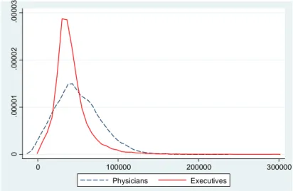
Using these two samples, it is possible to compare GPs’ and executives’ yearly income (…gure 1 and table 1). Remind that we use the same de…nition of income for the two samples: for GPs and executives, it corresponds to the annual level of income net of all contributions, and before income tax. It is worth noting that for the entire analysis, we are forced to adopt an unusual strategy to study incomes: we do not distinguish full-time from part-time workers and we do not measure full-time equivalent incomes. Indeed, these two variables (part time/full time and number of days worked during the year) are available for executives and not for GPs. Hence our income comparison will take as given the unobserved work duration chosen by each individual, which reinforces the retrospective nature of our analysis.

Table 1 and …gure 1 show that GPs’ income are higher than executives’: over the 1980-2004 period, the median income is 47,228e for GPs and 37,444e for executives. GPs’income are higher than executives’at nearly all points of the distribution, except at the bottom. Indeed, we …nd that the proportion of GPs with "low" income is higher than for executives and that the value of the …rst decile of income is higher for executives. The same pattern can be found at the very top of the distribution: while sector 1 GPs’ income are necessarily limited (given …xed fees and a theoretical maximum of 24 hours of work per day), this is not the case for executives. Figure 1 shows a higher proportion of

6_{Note that these surveys cannot be used for our study as individuals are followed for a maximum of}

Table 1: Distribution of income for physicians and executives D1 Q1 Median Q3 D9 Physicians 15,585 30,038 47,228 69,023 88,076 Executives 21,282 28,969 37,444 49,046 66,327

executives with high levels of income. However, despite of what is observed at the bottom and top of the distribution, GPs earn more than executives.

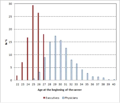
But the relevance of such a comparison pertinent can be questionned since it doen’t take into account that GPs are older than executives over the 1980-2004 period because of di¤erences in the demographic trends of the two professions (see below) and because they start working later (…gure 2). GPs begin their career between the ages 25 and 40, while executives begin between the ages 22 and 27 years old. This di¤erence in age at the beginning of the career re‡ects di¤erences in the duration of studies. Comparing GPs and executives’income should therefore control for the di¤erence of composition (by age) of the two professions and should take into account this di¤erence in the length of studies. More precisely, GPs and executives’ income should not be compared over the pooled 1980-2004 period but should be compared at each age to account for di¤erences in the characteristics of the two populations but also to take into account that di¤erences in income between the two professions may vary by age.

Figure 1: Distribution of physicians and executives’income (1980-2004)

0 .0 00 01 .0 00 02 .0 00 03 0 100000 200000 300000 Physicians Executives

Figure 2: Distribution of age at the beginning of the career for physicians and executives

4.2

Allowing for di¤erences in length of studies

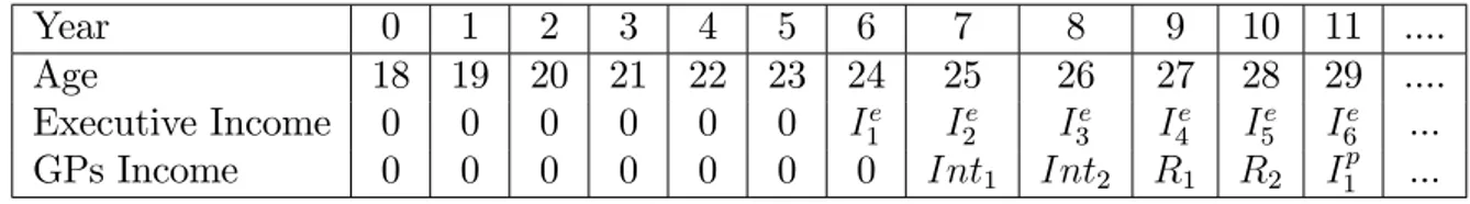
Table 2 describes two examples of trajectories of individuals who decide to become GPs or executives at the end of high school, when they are 18 (year 0).

Suppose that an individual decides to become an executive. In general, the duration of his studies is about 5 years and he begins his career at the age of 24. His income is denoted Ie, where e denotes that he is an executive. In practice, executives can begin their career some years later, especially because of grade repetition or failure to competitive exams, or because they experience di¢ culties in …nding a job and obtain only work placements. Table 2 provides an example, but there is a large variability of situations in our data.

Consider now an individual who decides to become a doctor. The duration of his studies is longer than for an executive: about 6 years in medical schools and 1 to 3 addi-tional years (depending on the time period) that are divided between medical school and training (called "medical internship"). More precisely, a typical trajectory for a GP is the following: he earns no income during the …rst six years, then he gets a small remuneration for his internship (that lasts 2 years in our example: Int1 and Int2). After graduation, GPs usually do not begin practicing as self-employed, but replace some doctors during holidays or short periods. During these periods, that can last several years (two years in our example), they earn incomes, denoted R1; R2; :::: Finally, GPs begin their own practice and earn their …rst income I₁p;where 1 denotes the …rst year of practice and p that he is a GP. In our example, the GP begins his practice at the age of 29, i.e. 5 years after an executive.

This …ve years di¤erence in the duration of studies and therefore in the age from which GPs and executives start having an income must be taken into account when comparing GPs and executives’ wealth, i.e. when cumulating their incomes over time. Therefore, our methodology will consists in comparing GPs and executives’ wealth from the age

Table 2: Summary ofthe beginning of careers of GPs and executives

Year 0 1 2 3 4 5 6 7 8 9 10 11 .... Age 18 19 20 21 22 23 24 25 26 27 28 29 .... Executive Income 0 0 0 0 0 0 I₁e I₂e I₃e I₄e I₅e I₆e ... GPs Income 0 0 0 0 0 0 0 Int1 Int2 R1 R2 I1p ...

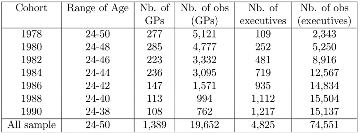
of 24, the theoretical age at which executives begin working 7_{. The year a GP or an} executive turned 24 will be de…ned as a "cohort". For GPs, available cohorts (de…ned by the year a GP turned 24) were all cohorts 1976 to 2000 whereas, for executives, available cohorts were only even cohorts from 1978 to 20048_{. To select a common set of cohorts,} each one containing at least 100 individuals (to perform a robust statistical analysis), seven cohorts were selected: 1978, 1980, 1982, 1984, 1986, 1988 and 1990. The number of observations per cohort is provided in table 3. As stated above, we restricted our samples to beginners and GP and executive earnings are recorded over the 1980-2004 period. Hence, our individuals are not observed over the same portion of lifetime. Individuals who belong to the 1978 cohort are observed until a maximum age of 50 years whereas individuals who belong to the 1990 cohort are observed until a maximum age of 38 years, as shown in table 3.

In the following, we consider two de…nitions of income.

The income earned from the beginning of the career, denoted I. Here the career is de…ned by the entrance on the labor market (and the …nding of a job) for the salaried executive and by the setting up of his/her practice by the GP, much later because of the extra duration of medical studies and of replacements. Refering to the examples provided in table 2, this income is Ie

1 ; I2e ; I3e ; I4e ; I5e ; I6e ; :::received from year 6 on by the executive. As for the GP, it is I1p; :::received from year 11.9 To compare the values of GP and executive trajectories, we have to accumulate in-dividuals’yearly incomes, with taking the same age as starting point. Hence we have to encompass a part of the individuals’educational trajectories. For this purpose, we consider another de…nition of income ‡ow, that starts from the age of 24 and that we denote Inc: Refering to the examples of table 2: from the age of 24 on (year 6), the ‡ow of income received by the executive is Inc = I1e ; I2e ; I3e ; I4e ; I5e ; I6e ; :::; and the ‡ow of income received by the GP is Inc = 0 ; Int1 ; Int2 ; R1 ; R2 ; I1p ; ::: In other word, to take into account the di¤erences in the duration of their studies, GP and executive wealths are compared from the age of 24.

7_{Actually, we observe the age of career start. Of course, all executives do not begin their career at}

24; part of them start later, for example at the age of 26. In that case, the individual income is set to 0 from 24 to 26 years old. On the contrary, very few executives begin their career before the age of 24, at 22 years old for example. In that case, our main results are obtained considering only the income earned from the age of 24. In a sensitivity analysis, we also include the income earned before the age of 24.

8_{Recall that salaried workers who are in our dataset are born in october of an even year.}

9_{Of course, these are particular …gures taken as examples: in our data we observe exactly at what}

Table 3: Number of observations per cohort

Cohort Range of Age Nb. of Nb. of obs Nb. of Nb. of obs GPs (GPs) executives (executives) 1978 24-50 277 5,121 109 2,343 1980 24-48 285 4,777 252 5,250 1982 24-46 223 3,332 481 8,916 1984 24-44 236 3,095 719 12,567 1986 24-42 147 1,571 935 14,834 1988 24-40 113 994 1,112 15,504 1990 24-38 108 762 1,217 15,137 All sample 24-50 1,389 19,652 4,825 74,551

4.3

The cohort pyramids

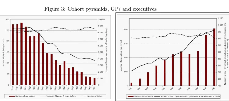
Figure 3 displays the "cohort pyramids" of GPs (on the left hand side) and executives (on the right hand side)10_{. Each cohort is de…ned by the year an individual turned 24. These} pyramids show very di¤erent patterns. On the right hand side, the number of executives per cohort has been growing rapidly and continuously from 1978 on, which results from the increase in the number of students with high skilled diploma (black line) but not from demographic changes: the number of births 24 years before the year considered (dotted line) is very stable accross the cohorts11_.

On the contrary, the number of GPs has decreased continuously from 1978 on. This pattern can be explained by the evolution of the numerus clausus 5 years before, which is the number of students allowed to go on with their medical education at the end of their …rst year of medicine. The variation of the numerus clausus is represented with the black line; introduced in 1971, it remained fairly constant until the end of the seventies (i.e. for GPs belonging to cohorts 1982 and before). Then, a restrictive policy was implemented, which resulted in a sizeable reduction in the numerus clausus (see Dormont and Samson [2008] for more details.

Table 4 presents the main characteristics of two cohorts, 1980 and 1990 for GPs and executives. Both professions experienced a large increase in the proportion of women. For individuals who belong to the 1990 cohort, nearly 44% of GPs are women and 28% of executives are women. Due to di¤erences in the demographic trends of the two professions (cf. …gure 3), over the 1980-2004 period, GPs are older than executives (GPs belonging to the 1990 cohort are 34.5 years old on average versus 31.3 for the executives of the same cohort). However, given a higher duration of studies for GPs, they also have a lower level of experience (4.7 years versus 7.1 for executives in the 1990 cohort). Again, whatever cohort is considered, GPs’ income is, on average, higher than executives’. Individuals belonging to the 1990 cohort have a lower level of income than those of the 1980 cohort, mostly because di¤erences in the level of experience between the two cohorts are not taken into account.

10_{Note that these pyramids cover a larger range of cohorts than the one used for this analysis:}

1978-1998.

11_{Note that the French economic situation provides an explanation for the few atypical years of the}

graph. Indeed, the decrease in the number of executives between cohorts 1990 and 1992 can be explained by the huge increase in the unemployment rate of executives observed between 1993 and 1995. Conversely, the increase in the number of executives between cohorts 1994 and 1996 can be explained by the decrease in the unemployement rate between 1998 and 2001.

Table 4: Description of the cohorts

Variable Cohort GPs Executives % of women 1980 20.6 13.9 1990 43.7 27.9 Average Age 1980 38.9 37.5 1990 34.5 31.3 Average Experience 1980 9.7 11.3 1990 4.7 7.1 Average Income (e) 1980 53,189 44,598

1990 51,191 37,498

Figure 3: Cohort pyramids, GPs and executives

5

Econometric Analysis

The econometric analysis is performed, as it is usual, on yearly income earned from the beginning of the career. Refering to the examples provided in table 2, we consider for the executive the yearly incomes received from year 6 on, i.e; Ie

1 ; I2e ; I3e ; I4e ; I5e ; I6e ; :::; and for the GP only I₁p; :::received only from year 11 on, and analyze the determinants of di¤erences in income between GPs and executives.

5.1

Empirical Speci…cation

Consider Iict the log of income (in 2004 Euros) in year t of the individual i (doctor or executive) belonging to cohort c: Our speci…cation is the following:

Iict = a + Zit0 b + Xi0d + '(t) + e+ c+ uit (1) where uit = i + "it

i = 1; ::::N ; c = 1; :::; C; t = 1; :::; T i = doctor or executive

Vector X0

i includes constant variables. For physicians and executives, it includes gender and two dummies characterizing whether the individual experienced a tem-porary break or left prematurely the sample, during the part of his career observed in our data set.

Vector Z0it includes time-varying variables. For physicians and executives, it in-cludes 22 regional dummies, speci…c to the region of work. For executives, we also include variables speci…c to the …rm size, the activity sector as well as, depending on the speci…cations, the annual number of days worked and a dummy indicating whether the individual works part time or full time. In order to make both estima-tions, on physicians and executives, comparable, our main speci…cation does not include these last two variables (which are not observed in the sample of physicians). '(t)is a quadratic function of time

e; e = 1; ::::; 25; are experience …xed e¤ects, where experience is de…ned as the number of years elapsed since the beginning of practice (in the examples of table 2, year 6 for the executive, and year 11 for the GP).

c; c = 1978; 1980; :::; 1990 (even years only) are cohort …xed e¤ects, where the cohort denotes the year the individual turned 24.

i is an individual speci…c e¤ect . For physicians, it could refer to their ability to attract and retain patients as well as their preference for leisure in the labour/leisure trade-o¤. For executives, it could refer to their intrinsic motivation, their ability to negociate their salary at the beginning of their career or their dynamism. "it is a disturbance that captures all events that lead physicians or executives to a decrease or an increase of their income at a given year. For physicians, it mainly refers to shocks of demand (transitory increase in demand for health care due to epidemics for example) or variations in the level of medical density in the same area of practice. For executives, it can refer to transitory, and volontary or not, periods of unemployment.

Model (1) includes experience, cohort and time e¤ects. In the literature, it is widely known that this kind of speci…cation generally raises identi…cation issues (see for example Deaton [1997]). Here we avoid such identi…cation problems because we use a quadratic function of time and, above all, because of our de…nition of cohort and experience, to-gether with variability in age of career beginning. Indeed, cohort is de…ned as the year the individual turned 24 while experience is de…ned as the number of years elapsed since the beginning of the career, which is de…ned, for executives by the …rst year he gets a real wage and for GPs, by the …rst year he sets up his practice (in examples of table 2, these are year 6 and 11, respectively, for the executive and the GP). Because age at

the beginning of the career varies considerably between individuals (see …gure (2)) and among one cohort, this prevent any colinearity between time, cohort and experience.

It is also important to underline that the structure of the sample is in‡uenced by the fact that we selected beginners. In 1980, all individuals have 1 year of experience; in 1981, the sample is composed of the same individuals, who then have 2 years of experience as well as new individuals who begin their career this year and who have 1 year of experience; and so on until 2004. The level of experience increases by 1 each year but the identi…cation between the experience and the time e¤ect is made possible by the fact that there beginners every year. Note however that the time e¤ects must be interpreted with caution: they represent the evolution of income over the 1980-2004 period for individuals who began their practice between 1980 and 2004 (and not for the whole population of physicians or executives who work during the 1980-2004 period).

Model (1) is a random e¤ect model estimated by feasible generalized least squares. This estimator is consistent as long as variables X0

i and Zit0 are uncorrelated with the error term. In our case, some variables, like the regional dummies, or the variables indicating a transitory break or a permanent leave are likely to be endogeneous ; the Hausman test for …xed e¤ects leads to the rejection of the null hypothesis that the random-e¤ect model provides consistent estimates. However, we prefer this speci…cation over a within speci…cation, that provides consistent estimates even when the explanatory variables are correlated with the individual speci…c component of the perturbation, i, but that would unable us to identify the e¤ect of most of our variables (most of them are constant over time, such as the cohort e¤ect, or have very little variation over the years).

Note that our estimates may be a¤ected by a selection biais. Indeed, as mentionned in section 3 ("data"), less than 2% of executives and GPs experience a temporary break or leave the sample prematurely. However, because these individuals leave the sample for various reasons, that are not observed in the dataset, we cannot deal with this problem by using Heckman’s selection model: participation in the sample cannot be speci…ed by a single participation equation. Following Verbeek and Nijman (1992), we simply added 2 dummies in each of the regression, indicating whether the GP or the executive left prematurely the sample or experienced a temporary break. This procedure does not correct for attrition biais, but it allows to test for its existence. Our estimates show that these dummies are jointly signi…cant and negative, suggesting that individuals who are in this situation have lower earnings. However, our main …ndings are probably una¤ected by a selection bias: the estimates are not a¤ected by the introduction of these participation dummies (probably because very few individuals are concerned).

5.2

Results

The estimated cohort, experience and time e¤ects are presented on …gures (4), (5) and (6). The other estimated coe¢ cients are presented in table A1 in the appendix. We mainly concentrate on the interpretation of the experience and cohort e¤ects.

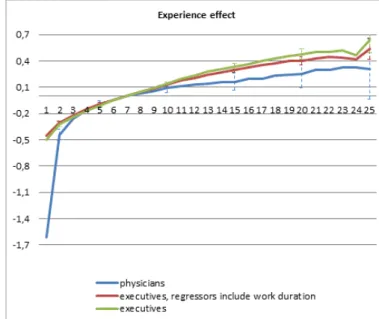
Figure 4 shows that, for both physicians and executives, income is an increasing and concave function of experience. However, at the beginning of the career (between 1 and 5 years), the pattern of physicians’ career pro…le is much steeper than the one of executives. During these years, physicians are characterised by a process of patient recruitment and their income grows rapidly. After 10 years of experience, physicians’

career pro…le becomes ‡atter than executives’. This di¤erence is consistent with Lazear and Moore (1984) prediction of a ‡atter earnings-pro…le for self-employed workers, who do not need productivity incentives as salaried workers.

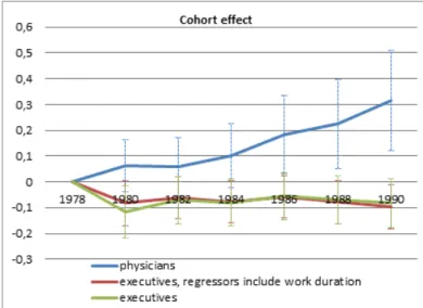
Cohort e¤ects (…gure 5) are very di¤erent between physicians and executives. For physicians, cohort e¤ects increase over the years. On the part of the career observed in our data set, physicians belonging to the 1980 cohort earn, on average 5% more than those belonging to the 1978 cohort (the reference category); those belonging to the 1984 cohort earn 10% more and those belonging to the 1990 cohort earn 30% more than the reference category. On the contrary, cohort e¤ects for executives exhibit a much ‡atter pro…le (most cohort e¤ects are not signi…cantly di¤erent from 0) and are even slighlty decreasing over the years.

What factors could explain such di¤erences in the two pro…les? Indeed, individuals belonging to the same cohort have turned 24 during the same year. Therefore, executives who belong to one cohort have experienced the same demographic context at the begin-ning of their career (the same unemployment rate and the level of competition between a given number of high-skilled individuals entering the labour market). Physicians who belong to one cohort have faced the same numerus clausus 6 years before or face the same demographic context at the beginning of their career about 6 years later. There-fore, the pattern of the cohort e¤ect is strongly driven by the evolution of the number of students with high-skilled diploma (for executives) and by the numerus clausus (for physicians). Comparing …gure (5) and (3), one can interpret these cohort e¤ects. The increase in income over the years for physicians can be explained by the decrease in the numerus clausus: less competition for patients between beginners favors higher income at the beginning of the practice but also throughout the career (see Dormont and Samson [2008] for more details). The contrary occurs for executives: a higher degree of competition between individuals arrving on the labor market at the same time prevents any cohort-linked increase in income.

The quadratic function of time shows an increase in income for both physicians and executives over the 1980-2004 period.

Table A1 in the appendix present the other estimated coe¢ cients. For executives, men earn 19% more than women, a gap consistent with the one found in di¤erent studies that measure the gender gap in pay for salaried workers when controlling for various explanatory variables such as experience, …rm sector of activity, …rm size, etc. (Meurs [2014]). As it is generally found in the literature, a rather small proportion of gender gap for executives can be ascribe directly to work duration: when we do not control for the number of days worked per year and the part time/full time dummy, the executive gender gap reaches 21%. As shown by Goldin [2014], however, this does not preclude that there is a large penalty in pay for women who ask for ‡exible schedules. As for physicians, men earn 41% more than women. Since our sample concerns sector 1 physicians, with …xed fees, this gender gap in pay re‡ects entirely di¤erent level of activity, i.e. a di¤erent number of consultations, each of whom is paid the same, whatever the GP’s gender.

We estimated equation (1) separately for men and women. Cohort e¤ects are very similar between men and women, for both physicians and executives. Experience e¤ects are very similar for male and female physicians, but di¤er slightly between male and female executives, with higher returns for women than for men.

Equation (1) also controls for regional dummies and, for executives only, for sectorial dummies or size of the …rm.

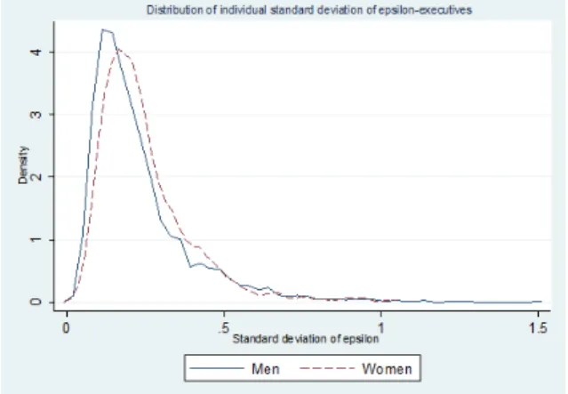
From speci…cation (1), we computed ("i), which is the individual standard deviation of the disturbance "it. More precisely, it represents the "within individual career" level of variability in income, once controlling for all explanatory variables (the experience and cohort e¤ects in particular). For physicians, part of this variability can be chosen (it can result from decisions to work more or less at a given year), or can be exogeneous (a transitory increase or decrease in demand, a variation in the level of medical density). For executives, this variability can also be chosen or constrained (it can refer to transitory, and volontary or not, periods of unemployment). The average level of individual variability is always higher for physicians (0.327) than for executives (0.237). This suggests that physicians have much more ‡exibility in their allocation of time throughout their career. Moreover, on average, this variability is, whatever the profession considered, always higher for women than for men: among physicians, it reaches 0.366 for women but 0.312 for men ; among executives, the gap is smaller: the average level of variability is 0.253 for women and 0.232 for men. This also suggests more variability in women’careers, and especially in female physicians’careers. The distribution of ("i)separately for men and women, is presented on …gure (7) for physicians and on …gure (8) for executives. For both professions, the distribution of ("i) for women is clearly on the right of that of men, meaning that a higher proportion of women experience a high level of variability during their career.

To sum up, this econometric analysis shows that GPs and executives have quite dif-ferent career pro…les. They suggest that GPs have more freedom in the allocation of their working time over their life. Their income are also favored by a low level of numerus clausus.

Figure 5: Cohort e¤ects for doctors and executives

Figure 6: Time e¤ects for doctors and executives

Figure 8: Distribution of individual standard deviation of epsilon - Executives

6

Comparison of wealth distributions

To compute wealth for each individual in accumulating all his/her yearly incomes, we have to take the same age as starting point. While econometric estimates were performed on income from the beginning of the career (I), we now consider income from the age of 24 on, that we denote Inc: As an illustration, the reader can refer to the examples provided in table 2: from year 6 on, the ‡ow of income received by the executive is Inc = Ie

1 ; I2e ; I3e ; I4e ; I5e ; I6e ; :::; and the ‡ow of income received by the GP is Inc = 0 ; Int1 ; Int2 ; R1 ; R2 ; I

p

1 ; :::This de…nition of income encompass a part of individual’s educational trajectory: it includes zeros for executives who start their career older than 24. As concerns doctors, it takes into account their longer education, with zero incomes until year 6 and small revenues from internship and replacements afterwards, before they set up their practice and perceive their …rst income I₁p (table 2): A stated above, considering this de…nition of income ‡ow enables us to take di¤erences in the duration of education into account when building wealth.

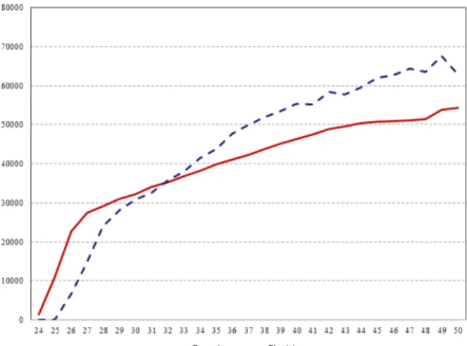
Figure 9 displays for GPs and executives the values of median incomes (Inc) by age. It shows that the median income of GPs is lower than the one of executives until the age of 32. Afterwards, GP median income is higher, which might enventually provide a pay-o¤ for their higher investment in education.

Wealth is de…ned as follows:

Wj(a) = a X =24 1 (1 + r) Inc j ; (2)

with j = e (executives) or p (physicians). r is a discount rate set at 3 %, with alternative hypotheses of 1% or 5 %. We consider a de…nition of wealth Wj_{(a)for di¤erent} ages. Of course, the appropriate concept for comparing careers is wealth over lifetime. However, we know that doctors are likely to earn less than executives at young ages because of their longer studies. If this higher investment in education is at some point paid o¤, it can be informative to compare wealth at di¤erent ages. Notice that the composition of the samples varies when we consider di¤erent ages for wealth computation: while age span lies between 24 and 50, recent beginners are not observed beyond the age of 38 (see table 3).

We compare the GP and executive wealth distributions with stochastic dominance analysis to examine if it pays to be a GP. Stochastic dominance analysis o¤ers the possi-bility to compare and order earnings distributions. Indeed, information about mean and variance of wealth is not su¢ cient: under the veil of ignorance, the individual aiming at choosing between GP and executive career does not know at which place of wealth distribution he/she would be situated. Following the methodology set up by Davidson and Duclos [2000] and used by Lefranc et al [2004], we ran non-parametric tests of stochastic dominance between GP and executive wealth distributions.

If people with requested ability can choose freely between a GP and executive career, long run equilibrium should imply a higher return to study for GPs that compensate their higher investment. Consequently wealth distributions should not di¤er signi…cantly at the equilibrium between executives and GPs.

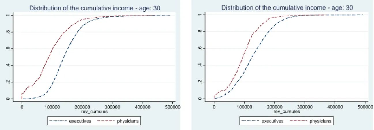
The stochastic dominance analysis was performed for men and women separately, and for wealth computed at age 30, 40 and 48. The cumulative distributions of wealth are given in graphs 10, 11 and 12. When wealth is computed at the age of 30, we …nd that the wealth distribution of executive dominates GP distribution at the …rst order for men and women. When people are 40, executive distribution of wealth still dominate GP distribution of wealth, but at the second order only, for men and women. At the age of 48, which is the oldest age we can consider, the results di¤er between men and women: on the one hand, GP and executive distributions of wealth are not anymore signi…cantly di¤erent for men; on the other hand, GP wealth distribution dominates executive wealth distribution at the …rst order for women.

These results show that the pay-o¤ for higher investment in education implied by medical studies takes a non negligible amount of time to be e¤ective: it is not yet realized at the age of 40. At the age of 48, we …nd that it is more pro…table for a woman to be a self-employed GP than a salaried executive, whereas there is no monetary advantage or disadvantage to be a GP rather than an executive for a man.

Figure 9: Annual level of income, including zeros for education and small revenues from intership and replacements (median by age)

Figure 10: Comparison of wealth distributions at the age of 30 0 .2 .4 .6 .8 1 0 100000 200000 300000 400000 500000 rev_cumules executives physicians

Distribution of the cumulative income - age: 30

Men-wealth at age 30 0 .2 .4 .6 .8 1 0 100000 200000 300000 400000 500000 rev_cumules executives physicians

Distribution of the cumulative income - age: 30

Women-wealth at age 30

Figure 11: Comparison of wealth distributions at the age of 40

0 .2 .4 .6 .8 1 0 500000 1000000 1500000 rev_cumules executives physicians

Distribution of the cumulative income - age: 40

Men-wealth at age 40 0 .2 .4 .6 .8 1 0 500000 1000000 1500000 rev_cumules executives physicians

Distribution of the cumulative income - age: 40

Figure 12: Comparison of wealth distributions at the age of 48 0 .2 .4 .6 .8 1 0 500000 1000000 1500000 2000000 rev_cumules executives physicians

Distribution of the cumulative income - age: 48

Men-wealth at age 48 0 .2 .4 .6 .8 1 0 500000 1000000 1500000 2000000 rev_cumules executives physicians

Distribution of the cumulative income - age: 48

Women-wealth at age 48

7

Conclusion

Is it desirable to be a GP in France, or should the National Health Insurance raise the conventional fees? For men, our …ndings show that there is no monetary advantage or disadvantage to be a GP rather than an executive. To claim higher fees, GPs should prove to have speci…c disutility associated with their profession, for example, a higher number of hours of work. When compared with executives, however, it is not obvious that GPs work a longer time.

It is true that GPs have longer studies than executives. Our …ndings show that the pay-o¤ in terms of wealth, for their higher investment in education takes a non negligible amount of time to be e¤ective: it is not yet realized at the age of 40. But at the age of 48, the wealth distributions of male executive and GPs do not di¤er signi…cantly. Morevover, since the average GP income exceeds executive income from the age of 32 on, it is very likely that at older ages male GPs’wealth dominate male executives’wealth.

In France as in most other countries GPs are at the bottom of the distribution of physician income: in 2004, their average monthly income was about 5,000 e whereas it was 8,500 for all specialists. A monetary advantage would a fortiori be observed if we considered specialists.

Despite this already favorable situation, GPs succeeded recently in convincing the National Health Insurance that they were treated unfairly. The fees have been raised by 4.5% (2011) and the introduction of a P4P has induced an additional increase of GP income of about 7.6 % (2012). These measures will probably favor GPs over executives in the future.12

For women our …ndings show there is a clear monetary advantage to be a GP rather than an executive. At the age of 48, which is the oldest age we can consider, GP wealth distribution dominates executive wealth distribution at the …rst order for women. Is it only a monetary advantage which is at stake? Actually, being a self employed physician

12_{However, we observe strong cohort e¤ect linked to the evolution of the numerus clausus over the}

years. Given the recent increase in the numerus clausus, the relative advantage of GPs might be reduced in the future.

o¤ers the possibility to allocate the working time freely over the week and over life time. The sources of gender gap in pay are di¤erent if the income depends on the number of consultations with …xed fees or if it results from the processes of hiring, wage seting and promotion within the …rm. As shown by Goldin (2014), one source of gender gap in pay is a way to manage the personnel that result in earnings that are non linear with respect to hours. Executive is the kind of profession where earnings have a non linear relationship with respect to hours and where there is a high penalty for ‡exible schedule. On the contrary, being GP in sector 1 with …xed fees per consultation is close to the perfect linear-in-time earnings (even with …xed charges for the o¢ ce, etc.). Our …ndings show that women with abilities and a high level of human capital have a clear advantage to be a GP.

A current statement asserts that it is not attractive to be GP and that it explains the rise in the proportion of women. Our results show another story. It is equivalent for men to be executive or GP and it much more advantageous for women to be a GP. The relative return for medical studies is higher for women. Hence the strong increase in the share of women in medicine faculties.

8

References

Cutler, David M. and Dan P. Ly (2011). "The (Paper) Work of Medicine: Under-standing International Medical Costs", Journal of Economic Perspectives, Vol. 25, n 2; p. 3-35.

Davidson, Russell and Jean-Yves Duclos (2000). "Statistical inference for sto-chastic dominance and for the measurement of poverty and inequality", Econometrica, Vol. 68, p.1435–1364.

Deaton, Angus (1997). The Analysis of Household Survey: a Microeconometric Ap-proach to Development Policy. The John Hopkins University Press.

Dormont, Brigitte and Anne-Laure Samson (2008). "Medical demography and intergenerational inequalities in General Practitioners’earnings", Health Economics, Vol. 17, p. 1037-1055

Dormont, Brigitte and Anne-Laure Samson (2009). "Démographie médicale et carrières des médecins généralistes: les inégalités entre générations", Economie et Statis-tiques, Vol. 414, p. 3-30

Friedman, M. and Simon Kuznets (1945). Income from Independent Professional Practice. National Bureau of Economic Research: New-York.

Goldin, Claudia (2013). "A grand Gender Convergence: Its Last Chapter".

Ameri-can Economic Association Presidential Addres, http://scholar.harvard.edu/…les/goldin/…les/grandgenderconvergence.pdf Hamilton, Barton H. (2002). "Does enterpreneurship pay? An Empirical Analysis of

the Returns to self-employment", Journal of Political Economy, Vol. 108, n 3, p. 604-631 Ketel, Nadine, Edwin Leuven, Hessel Oosterbeek and Bas Van der klaauw (2013). "The returns to medical school in a regulated labor market: Evidence from ad-mission lotteries", Working Paper

Lazear, EP. and RL. Moore (1984). "Incentives, productivity, and labor con-tracts". Quarterly Journal of Economics, Vol. 99, p. 275–296.

Lefranc, Arnaud, Nicolas Pistolesi and Alain Trannoy ( 2004). "Le revenu selon l’origine sociale", Economie et Statistiques, Vol. 371, p. 49–82.

Moeurs, Dominique ( 2014). Hommes/Femmes: une impossible égalité profession-nelle?", Opuscule du CEPREMAP n 32:

Nicholson, Sean and Carol Propper (2012). "Medical Workforce" in Handbook of Health Economics Volume 2, ed. by M.V. Pauly, T. G. McGuire and P.P. Barros, North Holland, p. 873-925.

Verbeek, Marno and Theo Nijman (1992). "Testing for selectivity bias in panel data models", International Economic Review, vol. 33, p. 681-703

Weeks, William B., Amy E. Wallace, Myron M. Wallace and H. Gilbert Welch (1994). "A comparison of the educational costs and incomes of physicians and other professionals", New England Journal of Medicine, Vol. 330, n 18, p. 1280-1286

Weeks, William B. and Amy E. Wallace (2002). "The more things change: revisit-ing a comparison of educational costs and incomes of physicians and other professionals", Academic Medicine, Vol. 77, n 4, p. 312-319

Welch, Finnis (1979). "E¤ects of Cohort Size on Earnings: The Baby Boom Babies’ Financial Bust", Journal of Political Economy, Vol. 87, n 5, p. S65-S97

9

Appendix

Table A-1 - Regression Estimates - Random e¤ect model

Log(income) Log(income) Log(income)

GPs Executives (1) Executives (2)

Variables common to GPs and executives:

Experience effects See figure (4)

Cohort effects See figure (5)

Time trend See figure (6)

female -0.415*** -0.178*** -0.210*** (0.033) (0.011) (0.012) Champagne-Ardennes -0.113 0.043* 0.026 (0.100) (0.023) (0.028) Picardie 0.345*** -0.034** -0.012 (0.088) (0.016) (0.020) Haute Normandie 0.375*** -0.002 -0.028 (0.091) (0.016) (0.020) Centre 0.129* -0.024* -0.045*** (0.076) (0.013) (0.017) Basse Normandie -0.122 -0.079*** -0.128*** (0.104) (0.022) (0.027) Bourgogne 0.170** -0.060*** -0.047** (0.084) (0.018) (0.022) Nord 0.347*** -0.015 -0.003 (0.065) (0.011) (0.014) Lorraine 0.200*** -0.076*** -0.099*** (0.075) (0.019) (0.024) Alsace -0.042 -0.060*** -0.062*** (0.074) (0.014) (0.017) Franche-Comté 0.201** -0.014 0.003 (0.090) (0.017) (0.022) Pays de la Loire 0.271*** -0.069*** -0.071*** (0.061) (0.013) (0.016) Bretagne -0.026 -0.092*** -0.097*** (0.062) (0.015) (0.019) Poitou Charentes 0.209** -0.131*** -0.150*** (0.085) (0.020) (0.025) Aquitaine 0.133** -0.070*** -0.074*** (0.063) (0.014) (0.018) Midi Pyrénées 0.067 -0.107*** -0.107*** (0.067) (0.010) (0.012) Limousin 0.061 -0.074** -0.068* (0.108) (0.029) (0.036) Rhône Alpes -0.085 -0.038*** -0.045*** (0.057) (0.006) (0.008) Auvergne 0.226** -0.026 -0.050* (0.101) (0.023) (0.028) Languedoc Roussillon 0.017 -0.118*** -0.128*** (0.068) (0.019) (0.023) PACA -0.086 -0.059*** -0.060*** (0.055) (0.010) (0.012) Corse -0.388* -0.253* -0.337** (0.209) (0.133) (0.161) Temporary break -0.278*** -0.014 -0.052*** (0.036) (0.009) (0.010) Leave Prematurely -0.233*** -0.029*** -0.105*** the sample (0.042) (0.011) (0.012) Variables specific to GPs: MEP Physicians -0.027 - -(0.031) Years between PHD and

1rst year of practice

0.009 (0.008)

Variables specific to Executives: Log(number of days worked) - 0.695*** (0.004) -Full time work - 0.292***

-(0.006) Firm size [50-99] - 0.038*** 0.044*** (0.006) (0.008) Firm size [100-199] - 0.031*** 0.058*** (0.006) (0.007) Firm size [200-499] - 0.024*** 0.061*** (0.005) (0.006) Firm size [500-1999] - -0.002 0.030*** (0.005) (0.006) Firm size [>2000] - -0.016*** 0.014** (0.005) (0.006) Agriculture - -0.305*** -0.212* (0.091) (0.113) Manufacture of food prod. - 0.042** 0.081***

(0.017) (0.022) Consumer goods industry - 0.019* 0.053***

(0.012) (0.014) Car industry - 0.028* 0.076***

(0.014) (0.018) Capital goods industry - 0.004 0.037***

(0.009) (0.011) Intermediate good industry - 0.028*** 0.059***

(0.010) (0.013) Energy - 0.059*** 0.112*** (0.015) (0.018) Construction industry - -0.004 0.005 (0.013) (0.016) Trade - 0.022** 0.045*** (0.010) (0.012) Transport - -0.018 0.024 (0.016) (0.020) Finance - 0.079*** 0.119*** (0.011) (0.014) Property business - -0.067*** -0.060** (0.022) (0.028) Business services - 0.013 0.027*** (0.008) (0.010) Education - -0.209*** -0.308*** (0.017) (0.021) Administration - -0.076*** -0.130*** (0.015) (0.019) Constant 10.452*** 6.222*** 10.608*** (0.081) (0.049) (0.048) Nb of Observations 17, 976 61, 002 61, 094 Standard errors in parentheses