HAL Id: pastel-00005275
https://pastel.archives-ouvertes.fr/pastel-00005275
Submitted on 21 Jul 2009
HAL is a multi-disciplinary open access
archive for the deposit and dissemination of sci-entific research documents, whether they are pub-lished or not. The documents may come from teaching and research institutions in France or abroad, or from public or private research centers.
L’archive ouverte pluridisciplinaire HAL, est destinée au dépôt et à la diffusion de documents scientifiques de niveau recherche, publiés ou non, émanant des établissements d’enseignement et de recherche français ou étrangers, des laboratoires publics ou privés.
time-dependent road networks
Giacomo Nannicini
To cite this version:
Giacomo Nannicini. Point-to-point shortest paths on dynamic time-dependent road networks. Com-puter Science [cs]. Ecole Polytechnique X, 2009. English. �pastel-00005275�
Point-to-Point Shortest Paths
on Dynamic Time-Dependent
Road Networks
Th`ese pr´esent´ee pour obtenir le grade de
DOCTEUR DE L’ECOLE POLYTECHNIQUE
par
Giacomo Nannicini
Soutenue le 18 juin 2009 devant le jury compos´e de:
Dorothea Wagner Universit¨at Karlsruhe, Karlsruhe Rapporteur Roberto Wolfler-Calvo Universit´e Paris Nord, Paris Rapporteur Gilles Barbier DisMoiO `u, Paris
Philippe Goudal Mediamobile, Ivry sur Seine Frank Nielsen Ecole Polytechnique, Palaiseau
Leo Liberti Ecole Polytechnique, Palaiseau Directeur de th`ese Philippe Baptiste Ecole Polytechnique, Palaiseau Co-directeur de th`ese Daniel Krob Ecole Polytechnique, Palaiseau Co-directeur de th`ese
3 Abstract
The computation of point-to-point shortest paths on time-dependent road networks has many practical applications which are interesting from an indus-trial point of view. Typically, users are interested in the path leading to their des-tination which has the smallest travel time among all possible paths; it is nat-ural to model the shortest paths problem on a time-dependent graph, where the arc weights are travel times that depend on the time of day at which the arc is traversed. We study both fully combinatorial methods and mathemat-ical formulation based methods. From a combinatorial point of view, if we impose some restrictions on the arc weights, the problem can be solved in polynomial time with the well known Dijkstra’s algorithm. However, apply-ing Dijkstra’s algorithm on a graph with several millions of vertices and arcs, such as a continental road network, may require several seconds of CPU time. This is not acceptable for real-time industrial applications; therefore, the need for speedup techniques arises. Bidirectional search is a standard technique to speed up computations on static (i.e. non time-dependent) graphs; however, as the arrival time at the destination is unknown, the cost of time-dependent arcs around the target node cannot be evaluated, thus bidirectional search can-not be directly applied on time-dependent networks. We propose an algorithm based on an asymmetric bidirectional search, which allows the extension to the time-dependent case of hierarchical speedup techniques, well known for static graphs. Our method deals efficiently with dynamic scenarios where arcs weights can change, so that we can take into account real-time and forecast traf-fic information as soon as it becomes available. We achieve average query times for time-dependent shortest paths computations that were previously only pos-sible on dynamic graphs with static arc costs. We discuss the integration of our algorithm with an existing real-world industrial application. For general arc weight functions, the problem is not polynomially solvable; we propose a mathematical programming formulation which is a Mixed-Integer Linear Pro-gram (MILP) if the time-dependent arc weights are linear or piecewise linear functions, whereas it is a Mixed-Integer Nonlinear Program (MINLP) if the arc weights are nonlinear functions. We study efficient algorithms for both classes of problems, and test them on benchmark instances taken from the literature, as well as shortest paths instances. We propose new branching strategies within the context of a Branch-and-Bound algorithm for MILPs. Computational ex-periments show that, by generating good branching decisions, we enumerate on average half the nodes enumerated by traditional strategies. Our approach is also competitive in terms of total computational time. Finally, we present a general-purpose heuristic for MINLPs based on Variable Neighbourhood Search, Local Branching, Sequential Quadratic Programming and Branch-and-Bound. Experiments show the reliability of our heuristic with respect to methods pro-posed in the literature.
Contents
1 Introduction 9
1.1 Motivation . . . 9
1.2 Definitions and Notation . . . 12
1.2.1 The FIFO property . . . 13
1.2.2 Choice of the cost functions . . . 13
1.3 Mathematical Programming Formulations for the TDSPP . . . 14
1.3.1 Definition of mathematical program . . . 15
1.3.2 Formulation of the TDSPP . . . 18
1.3.3 Analysis of the formulations . . . 20
1.4 Related Work . . . 21
1.4.1 Early history . . . 21
1.4.2 Dijkstra’s algorithm . . . 23
1.4.3 Label-correcting algorithm . . . 24
1.4.4 Hierarchical speedup techniques for static road networks . 26 1.4.4.1 Highway Hierarchies . . . 26
1.4.4.2 Dynamic Node Routing . . . 28
1.4.4.3 Contraction Hierarchies . . . 30
1.4.5 Goal-directed search: A∗ . . . 31
1.4.5.1 The ALT algorithm . . . 32
1.4.6 The SHARC algorithm . . . 33
1.5 Contributions . . . 35
1.6 Overview . . . 38
I
Combinatorial Methods
41
2 Guarantee Regions 45 2.1 Definitions and main ideas . . . 462.2 Computing the node sets . . . 49
2.3 Query algorithm . . . 51
2.4 Implementation . . . 53
2.4.1 Storing node sets . . . 53
2.4.3 Drawbacks of guarantee regions . . . 57
3 BidirectionalA∗Search on Time-Dependent Graphs 59 3.1 Algorithm description . . . 59
3.2 Correctness . . . 61
3.3 Improvements . . . 63
3.4 Dynamic cost updates . . . 66
4 Core Routing on Time-Dependent Graphs 69 4.1 Algorithm description . . . 69
4.2 Practical issues . . . 72
4.2.1 Proxy nodes . . . 72
4.2.2 Contraction . . . 73
4.2.3 Outputting shortest paths . . . 74
4.3 Dynamic cost updates . . . 74
4.3.1 Analysis of the general case . . . 75
4.3.2 Increases in breakpoint values . . . 75
4.3.3 A realistic scenario . . . 76 4.4 Multilevel Hierarchy . . . 77 5 Computational Experiments 79 5.1 Input data . . . 79 5.1.1 Time-dependent arcs . . . 80 5.2 Contraction rates . . . 81 5.3 Random Queries . . . 85 5.3.1 Local Queries . . . 92 5.4 Dynamic Updates . . . 93 6 A Real-World Application 97 6.1 Description of the existing architecture . . . 97
6.2 Description of the proposed architecture . . . 99
6.2.1 Load balancing and fault tolerance . . . 102
6.3 Updating the cost function coefficients . . . 104
II
Mathematical Formulation Based Methods
107
7 Improved Strategies for Branching on General Disjunctions 111 7.1 Preliminaries and notation . . . 1127.2 A quadratic optimization approach . . . 113
7.2.1 The importance of the norm ofλ . . . 117
7.2.2 Choosing the setRk . . . 118
7.2.3 The depth of the cut is not always a good measure . . . 119
CONTENTS 7
7.3.1 Generating a pool of split disjunctions . . . 124
7.4 Computational experiments: quadratic approach . . . 126
7.4.1 Comparison of the different methods . . . 127
7.4.2 Combination of several methods . . . 132
7.5 Computational experiments: MILP formulation . . . 139
8 A Good Recipe for Solving MINLPs 145 8.1 The basic ingredients . . . 146
8.1.1 Variable neighbourhood search . . . 146
8.1.2 Local branching . . . 147
8.1.3 Branch-and-bound for cMINLPs . . . 147
8.1.4 Sequential quadratic programming . . . 148
8.2 The RECIPE algorithm . . . 149
8.2.1 Hyperrectangular neighbourhood structure . . . 149
8.3 Computational results . . . 151
8.3.1 MINLPLib . . . 152
8.3.2 Optimality . . . 154
8.3.3 Reliability . . . 155
8.3.4 Speed . . . 155
9 Computational Experiments on the TDSPP 157 9.1 Input data . . . 157
9.2 Numerical experiments with the linear formulation . . . 159
9.2.1 Formulation . . . 159
9.2.2 Computational results . . . 160
9.3 Numerical experiments with the nonlinear formulation . . . 162
9.3.1 Formulation . . . 163
9.3.2 Modifications to RECIPE . . . 163
9.3.3 Computational results . . . 164
III
Conclusions and Bibliography
167
10 Summary and Future Research 169 10.1 Summary . . . 16910.2 Future research . . . 173
Chapter 1
Introduction
1.1
Motivation
Route planners and associated features are increasingly popular among web users: several web sites provide easy-to-use interfaces that allow users to select a starting and a destination point on a map, and a path between the two points satisfying one or more criteria is computed. Possible criteria are, for example: minimize travel time, total path length or estimated travel cost. Similar capa-bilities can be found in GPS devices; as these usually have a limited amount of memory and CPU power, several devices now use different kinds of wireless connections in order to query a web service, which computes the desired path using more sophisticated algorithms than those available on the portable de-vice.
Users are typically interested in the fastest path to reach their destination, i.e. the shortest path in terms of travel time. However, usually only static infor-mation is taken into account when computing this kind of shortest paths, while it is well known that the travel time over a road segment depends on its conges-tion level, which in turn is dependent on the time instant at which the road segment is traversed. This implicitly requires complete knowledge of both real-time and forecast traffic information over the whole road network, so that we are able to compute the traversal time of a road segment for each time instant in the future. This assumption is obviously unrealistic; nevertheless, several statistical models exist which are able to predict to a certain degree of accuracy the evolution of traffic. This kind of analysis is made possible by traffic sensors (electromagnetic loops, cams, etc.) that are positioned at strategic places of the road network and constantly monitor the traffic situation, providing both high-level information such as the congestion level of a highway and low-level information such as the travel time in seconds over a particular road segment. Using a large database of historical traffic information and statistical analysis tools we can compute speed profiles for the different road segments, i.e. cost functions that associate the most probable travel speed (and thus travel time)
over a road segment with the time instant at which the segment is traversed. Typically there will be several classes of these speed profiles, e.g. one class of profiles for weekdays and another one for holidays. A road network such that the travel time over a road segment depends on the time instant at which the segment is traversed is called time-dependent. One practical problem arises: as road networks may be very large, traffic sensors cannot cover all road seg-ments. In real-world scenarios, only a small part of the road network is con-stantly monitored, while the remaining part is not covered by sensors and, as a consequence, by speed profiles. However, the monitored part of the road net-work corresponds to the most important road segments, e.g. motorways and highways. For long distance paths, the traffic congestion status of these seg-ments is the most important for determining the total travel time, and is also the most significant from a user’s point of view: it is reasonable to assume that a car driver which asks for the fastest path to reach the destination wants to avoid traffic jams on high importance roads, which have a large influence on the total travel time, while congestions at local level near the departure or the destination point are less important, as well as more difficult (if not impossible) to foresee. Thus, in a realistic situation only a part of the road network is pro-vided with real-time and forecast traffic information, while the remaining part is associated with static travel times.
This scenario is further complicated by the fact that the speed profiles may not be the most accurate traffic information available. Indeed, it is clear that real-time information, as detected by the traffic sensors, gives the best estima-tion of travel times for the time instant at which it is gathered. Moreover, sev-eral predictive models for short and mid-term traffic forecasting exist, which are beyond the scope of this work and will not be discussed here; these mod-els are based on the real-time information and capitalize on the temporal and spatial locality of traffic jams, so that they are able to predict congestions with a larger degree of accuracy with respect to speed profiles, which only take into account historical data. In the end, the historical speed profiles are not the only source of traffic information: they provide a good estimation of long term traf-fic dynamics, but for short and mid-term forecasting more accurate dynamic data is available. Therefore, the cost functions that associate travel times to road segments and the time at which the segment is traversed should ideally be dynamic, i.e. they should be based on historical speed profiles, but they should be frequently updated in order to take into account both real-time traf-fic information and short and mid-term traftraf-fic forecastings. In the following we will assume that the time required for each shortest path computation is much shorter than the time interval at which real-time traffic information (and thus traffic forecastings) is updated, so that computations can always be carried out before the cost functions are modified. This is realistic in industrial applica-tions, since a shortest path should be computed very quickly (no more than a second), whereas traffic information is typically updated every few minutes.
1.1 Motivation 11
Under reasonable assumptions, the problem of finding the shortest path in terms of travel time on a time-dependent road network is theoretically solved in polynomial time by Dijkstra’s algorithm (see Section 1.2.1 and Section 1.4.2). However, an application of Dijkstra’s algorithm over a continental sized road network may require several seconds of CPU time, and in several real-world scenarios this may be too long. For instance, consider the web service scenario: if we assume that there may be several shortest path queries per second, then each shortest path computation should take no more than a few milliseconds. This situation also arises in the case of GPS devices: real-time and forecast traf-fic information may be diftraf-ficult to deliver to limited capabilities devices for several reasons (bandwidth, secrecy, etc.), so that the most efficient choice is gathering the traffic information on a server machine with large computational power, which should then quickly provide answers to shortest path queries to all connected devices. This motivates our need for speedup techniques. It is easy to develop heuristic strategies, e.g. for long distance paths we can restrict the search to motorways after a few kilometers away from the starting point, thus neglecting all less important roads. However, both from a theoretical and a practical point of view we are more interested in exact methods, or at least methods with a (small) approximation guarantee. While in other shortest paths applications only exact solutions may be interesting, a small approximation fac-tor is practically acceptable when dealing with road networks, since the input data (i.e. travel times) is affected by measurement errors anyway, and traffic forecasts may fail to be exact.
In the general case, i.e. without restrictions on the cost functions, the time-dependent shortest path problem is NP-hard (see Section 1.2.1). For very large networks, there is no hope of solving it to optimality within a short time; there-fore, for real-time applications we are more interested in a restriction of the problem which is polynomially solvable. However, the study of the general case finds application as a mean to verify that the solutions to the polynomially solv-able restriction of the problem are meaningful for the network users, even when the restrictions are lifted. We model the time-dependent shortest path problem in a general network through a mathematical program. The greatest advantage of employing a mathematical program is the flexibility of the resulting model: we can choose arbitrary cost function, and easily add complicating constraints that would be difficult to satisfy with a Dijkstra-like approach. For instance, taking into account prohibited turnings is straightforward within the mathe-matical programming formulation that we propose. This program is a mixed-integer linear program or a mixed-mixed-integer nonlinear program, depending on the functions which model the travelling time over the arcs of the network. In-stead of searching for specialized algorithms to solve the time-dependent short-est path problem in the general case, we study general-purpose algorithms for mixed-integer linear programs and mixed-integer nonlinear programs. This al-lows us to improve the performance with respect to the literature of existing
algorithms that solve very large classes of problems, one of which is the routing problem that is the specific subject of this thesis.
1.2
Definitions and Notation
Consider an intervalT = [0, P ] ⊂ R and a function space F of positive functions f : R+ → R+ with the property that ∀τ > P f (τ ) = f (τ − kP ), where k =
max{k ∈ N|τ − kP ∈ T }. This implies f (τ + P ) = f (τ ) ∀τ ∈ T ; in other words,f is periodic of period P . We additionally require that f (x) + x ≤ f (y) + y ∀f ∈ F, x, y ∈ R+, x ≤ y; this ensures that our network respects the FIFO
property when the functions are interpreted as travel times (see Section 1.2.1). The juxtapositionf ⊕ g of two functions f, g ∈ F is a function ∈ F defined as (f ⊕ g)(τ ) = f (τ ) + g(f (τ ) + τ ) ∀τ ∈ R+. Note that this operation is neither
commutative nor associative, and should be evaluated from left to right; that is, f ⊕ g ⊕ h = (f ⊕ g) ⊕ h. The minimum min{f, g} of two functions f, g ∈ F is a function∈ F such that (min{f, g})(τ ) = min{f (τ ), g(τ )} ∀τ ∈ T . We define the lower bound off as f = minτ∈T f (τ ), and the upper bound as f = maxτ∈T f (τ ).
Consider a directed graphG = (V, A), where the cost of an arc (u, v) is a time-dependent function given by a functionc : A → F; for simplicity, we will write c(u, v, τ ) instead of c(u, v)(τ ) to denote the cost of the arc (u, v) at time τ ∈ T . We defineλ, ρ : A → R+asλ = c and ρ = c, i.e. ∀(u, v) ∈ A λ(u, v) = c(u, v) and
ρ(u, v) = c(u, v); we assign their own symbol to these two functions because they will be used very often in the following.
We denote the distance between two nodess, t ∈ V with departure from s at timeτ0 ∈ T as d(s, t, τ ). The distance function between s and t is defined as
d∗(s, t) : T → R+, d∗(s, t)(τ ) = d(s, t, τ ). We denote by Gλthe graphG weighted
by the lower bounding functionλ; the distance between two nodes s, t on Gλis
denoted bydλ(s, t). Similarly, we denote the graph G weighted by ρ as Gρ.
Given a pathp = (s = v1, . . . , vi, . . . , vj, . . . , vk = t), its time-dependent cost is
defined asγ(p) = c(v1, v2) ⊕ c(v2, v3) ⊕ · · · ⊕ c(vk−1, vk). Its time-dependent cost
with departure time atτ0 ∈ T is denoted as γ(p, τ0) = γ(p)(τ0). We denote the
subpath ofp from vi tovj byp|vi→vj. The concatenation of two pathsp and q is
denoted byp + q.
We callG the reverse graph of G, i.e. G = (V, A) where A = {(u, v)|(v, u) ∈ A}. ForV′ ⊂ V , we define A[V′] = {(u, v) ∈ A|u ∈ V′, v ∈ V′} as the set of arcs
with both endpoints inV′. Correspondingly, the subgraph ofG induced by V′is
G[V′] = (V′, A[V′]). We define the union between two graphs G
1 = (V1, A1) and
G2 = (V2, A2) as G1∪ G2 = (V1∪ V2, A1∪ A2).
We can now formally state the Time-Dependent Shortest Path Problem: TIME-DEPENDENTSHORTESTPATHPROBLEM(TDSPP): given a directed
graph G = (V, A) with cost function c : A → F as defined above, a source node s ∈ V , a destination node t ∈ V and a departure time
1.2 Definitions and Notation 13
τ0 ∈ T , find a path p = (s = v1, . . . , vk = t) in G such that its
time-dependent costγ(p, τ0) is minimum.
We will assume that our problem is to find the fastest path between two nodes with departure at a given time; the “backward” version of this problem, i.e. finding the fastest path between two nodes with arrival at a given time, can be solved with the same method (see (39)).
1.2.1
The FIFO property
The First-In-First-Out property states that for each pair of time instantsτ, τ′ ∈
T with τ′ > τ :
∀ (u, v) ∈ A c(u, v, τ ) + τ ≤ c(u, v, τ′) + τ′,
The FIFO property is also called the non-overtaking property, because it basi-cally says that ifT1 leavesu at time τ and T2 at timeτ′ > τ , T2cannot arrive at
v before T1 using the arc(u, v). Note that our choice of the function space for
the time-dependent arc cost function in Section 1.2 ensures that the FIFO prop-erty holds. Although FIFO networks are useful for the study of those means of transportation where overtaking is rare (such as trains), modelling of car trans-portation yields networks which do not necessarily have the FIFO property. For the TDSPP, the FIFO assumption is usually necessary in order to mantain an acceptable level of complexity: the SPP in time-dependent FIFO networks is polynomially solvable (85), even in the presence of traffic lights (5), while it is NP-hard in non-FIFO networks (117).
In Part I we will deal with time-dependent graphs for which the FIFO prop-erty holds. This is motivated by the fact that the real-world time-dependent data provided by the Mediamobile company1 consists in functions which
sat-isfy the FIFO property. However, at the beginning of this thesis this was not clear because data gathering and manipulation was still in progress. Hence, the parts of this work dealing with mathematical programming are motivated by the study of non-FIFO networks. The original idea was to consider only FIFO functions, so that the TDSPP is polynomially solvable, and to use a mathemati-cal programming formulation of the TDSPP on non-FIFO networks in order to verify the quality of the solutions found.
1.2.2
Choice of the cost functions
In order to implement an efficient algorithm for shortest paths computations on time-dependent graphs we must be able to efficiently carry out several op-erations between time-dependent functions, e.g.: computing the composition
and the minimum of two functions, obtaining lower and upper bounds (see Sec-tion 1.4.3). Moreover, the funcSec-tions should be as quick as possible to evaluate. The practical difficulty of dealing with time-dependent cost function depends on the complexity of the cost function (40). For real-time applications, we want to keep this difficulty as low as possible; thus, a natural choice is to use piece-wise linear functions to model arc costs, which allow for some flexiblity while being simple to treat algorithmically. Furthermore, piecewise linear functions have the advantage that the FIFO property can be easily enforced: it is straight-forward to note that the condition f (x) + x ≤ f (y) + y ∀x ≤ y translates to
df(x)
dx ≥ −1.
Although all theoretical considerations are valid for general cost functions, through the rest of this work when dealing with FIFO networks we will assume that from a practical point of view the time-dependent cost functions on arcs can be represented by piecewise linear functions. In particular, this holds through Part I.
When lifting the restrictions on the arc costs, a reasonable model to take into account perturbations due to traffic on an arc is to consider a constant cost, which represents the travelling time in traffic-free conditions, plus a summa-tion of Gaussian funcsumma-tions, each one centered on a traffic congessumma-tion. Formally, for each arc(i, j) ∈ A we have:
c(i, j, τ ) = cij + h X k=1 ake −(τ −µk)2 2σ2k ,
where cij is the travelling time over arc (i, j) in uncongested hours, and h is
the number of traffic congestions over one day. Each congestion is centered at timeµk, and has in practice no effect more than 3σk away from the mean
µk. Note that this cost function is not necessarily FIFO, thus we cannot employ
Dijkstra-like algorithms. Therefore, we will deal with it through a mathematical programming formulation.
1.3
Mathematical Programming Formulations for
the TDSPP
The TDSPP in FIFO networks can be efficiently solved in a combinatorial way, as we will see in Part I. However, it can also be modeled as a mathematical pro-gram, and solved with general-purpose methods for mathematical programs. This will be the subject of Part II. In this section we define a mathematical pro-gram that models the TDSPP with arbitrary cost functions.
The rest of this section is organized as follows. In Section 1.3.1 we give a definition of mathematical program taken from the literature, identifying differ-ent classes of mathematical programs. In Section 1.3.2 we give a mathematical
1.3 Mathematical Programming Formulations for the TDSPP 15
programming formulation for the TDSPP with arbitrary cost functions. In Sec-tion 1.3.3 the size of the proposed formulaSec-tions is analyzed, and a reasonable model for the cost functions is proposed.
1.3.1
Definition of mathematical program
Wikipedia2defines mathematical programming as:
[. . . ] the study of problems in which one seeks to minimize or maxi-mize a real function by systematically choosing the values of real or integer variables from within an allowed set. This (a scalar real val-ued objective function) is actually a small subset of this field which comprises a large area of applied mathematics and generalizes to study of means to obtain “best available” values of some objective function given a defined domain where the elaboration is on the types of functions and the conditions and nature of the objects in the problem domain.
Typically, mathematical programs are cast in the form: min f (x) subject to: ∀j ∈ M gj(x) ≤ 0 xL≤ x ≤ xU x ∈ X (P )
where X is a cartesian product of continuous and discrete intervals. In this case, we have a single objective functionf , a set M of constraints gj, a vector of
variable lower and upper boundsxL, xU, not necessarily finite. The meaning of
the mathematical program(P ) is that we seek, among all points x ∈ X which satisfiy the constraintsgj(x) ≤ 0 ∀j ∈ M , xL ≤ x ≤ xU, the one that yields the
smallest value off (x).
A formal definition of mathematical program is given in (93; 94). The def-inition is such that it easily translates into a data structure that can be imple-mented on a computer. Let P be the set of all mathematical programs, and M be the set of all matrices. We recall that, given a directed graphG = (V, A) and a nodev ∈ V , δ+(v) indicates the set of vertices u such that (v, u) ∈ A, and δ−(v)
denotes the set of verticesu such that (u, v) ∈ A. The definition of a mathemat-ical program given in (93; 94) is as follows.
Definition 1.3.1. Given an alphabetL consisting of countably many
alphanu-meric namesNL and operator symbols OL, a mathematical programming
for-mulationP is a 7-tuple (P, V, E, O, C, B, T ), where:
• P ⊂ NL is the sequence of parameter symbols: each element p ∈ P is a
parameter name;
• V ⊂ NLis the sequence of variable symbols: each elementv ∈ V is a variable
name;
• E is the set of expressions: each element e ∈ E is a DAG e = (Ve, Ae) such
that:
(a) Ve ⊂ L is a finite set
(b) there is a unique vertexre ∈ Vesuch thatδ−(re) = ∅ (such a vertex is
called the root vertex)
(c) verticesv ∈ Vesuch thatδ+(v) = ∅ are called leaf vertices and their set
is denoted byL(e); all leaf vertices are such that v ∈ P ∪ V ∪ R ∪ P ∪ M
(d) ∀v ∈ Ve : δ+(v) 6= ∅ ⇒ v ∈ OL
(e) two weight functionsχ, ζ : Ve → R are defined on Ve: χ(v) is the node
coefficient andζ(v) is the node exponent of the node v; for any vertex v ∈ Ve, we letτ (v) be the symbolic term of v: namely, v = χ(v)τ (v)ζ(v).
Elements ofE are sometimes called expression trees; nodes v ∈ OLrepresent
an operation on the nodes inδ+(v), denoted by v(δ+(v)), with output in R;
• O ⊂ {−1, 1} × E is the sequence of objective functions; each objective
func-tion o ∈ O has the form (do, fo) where do ∈ {−1, 1} is the optimization
direction (−1 stands for minimization, +1 for maximization) and fo ∈ E;
• C ⊂ E × S × R (where S = {−1, 0, 1}) is the sequence of constraints c of the
form(ec, sc, bc) with ec ∈ E, sc ∈ S, bc ∈ R: c ≡ ec ≤ bc if sc = −1 ec = bc if sc = 0 ec ≥ bc if sc = 1;
• B ⊂ R|V|× R|V|is the sequence of variable bounds: for allv ∈ V let B(v) =
[Lv, Uv] with Lv, Uv ∈ R;
• T ⊂ {0, 1, 2}|V| is the sequence of variable types: for allv ∈ V, v is called
a continuous variable if T (v) = 0, an integer variable if T (v) = 1 and a
binary variable ifT (v) = 2.
Given an expression tree DAGe = (Ve, Ae) with root node r(e) and whose leaf
nodes are elements of R or of M, the evaluation ofe is the numerical output of the operation represented by the operator node in noder applied to all nodes adjacent tor. For leaf nodes belonging to P, the evaluation is not defined; the
1.3 Mathematical Programming Formulations for the TDSPP 17
mathematical program in the leaf node must first be solved and a relevant op-timal value must replace the leaf. An algorithm to evaluate expression trees is given in (94).
Definition 1.3.1 states that a mathematical program consists in a set of vari-ables with an associated type and lower/upper bounds, a set of parameters, a set of equality/inequality constraints, and a set of objective functions, each one with an associated optimization direction (minimization/maximization).
Based on Definition 1.3.1, we distinguish several classes of mathematical programs. In this thesis, we are interested in the following categories.
• Linear Programs: a mathematical programming problem P is a Linear Program (LP) if|O| = 1, e is a linear form for all e ∈ E, and T (v) = 0 for all v ∈ V . In other words, a LP has only one objective value, linear objective function and constraints, and all variables are continuous. • Mixed-Integer Linear Programs: a mathematical programming problem
P is a Mixed-Integer Linear Program (MILP) if |O| = 1 and e is a linear form for alle ∈ E. In other words, a MILP has only one objective value, linear objective function and constraints, and variables can be both con-tinuous and discrete.
• Nonlinear Programs: a mathematical programming problemP is a Non-linear Program (NLP) if |O| = 1 and T (v) = 0 for all v ∈ V . In other words, a NLP has only one objective value and all variables are contin-uous, while the objective function and the constraints can be arbitrary linear/nonlinear expressions.
• Mixed-Integer Nonlinear Programs: a mathematical programming prob-lemP is a Mixed-Integer Nonlinear Program (MINLP) if |O| = 1. In other words, a MINLP has only one objective value; variables can be both con-tinuous and discrete, while the objective function and the constraints can be arbitrary linear/nonlinear expressions.
Within the class of NLPs (respectively, MINLPs), we distinguish between con-vex NLPs (MINLPs) ife represents a convex function for all e ∈ E, whereas it is a nonconvex NLP (MINLP) otherwise. In general, solving LPs and convex NLPs is considered easy, and solving MILPs, nonconvex NLPs and convex MINLPs (cMINLPs) is considered difficult. Solving nonconvex MINLPs involves diffi-culties arising from both nonconvexity and integrality, and it is considered the hardest problem of all.
A mathematical program may also have multiple objective functions, which adds to the complexity of the problem. In fact, in a mathematical sense it is not clear how a solution can be optimal with respect to more than one objective function, if these are conflicting. In this case, one is often interested in the set of non-dominated solutions, i.e. the set of Pareto optima. Intuitively, this
consists in the set of solutions such that each one is better than the other ones for at least one of the considered optimization criteria. However, in this work we are mainly interested in single objective optimization; we refer the reader to (55) for an introduction to multi-objective optimization.
1.3.2
Formulation of the TDSPP
We seek to derive mathematical programming formulations for the TDSPP un-der different assumptions. It is natural to start with a formulation for the short-est paths problem on static graphs, and then add time-dependency into the model. A classical formulation for the SPP (see (87)) is the following. LetM ∈ {−1, 0, 1}|V |×|A|be the incidence matrix ofG, i.e., a matrix whose element mv
ij is:
+1 ifv = i, i.e. if arc (i, j) is in the forward star of node v, -1 if v = j, and 0 other-wise. Supposecij is the cost of arc(i, j) ∈ A. We consider a network flow
prob-lem (4) with demandsbv = 1 for v = s, bv = −1 for v = t and bv = 0 ∀v ∈ V \{s, t}:
min P (i,j)∈Acijxij ∀v ∈ V P (i,j)∈Amvijxij = bv ∀(i, j) ∈ A xij ∈ {0, 1} (SP P )
This is equivalent to introducing one unit of flow at the source node, and requir-ing that this unit reaches the destination while passrequir-ing through arcs that mini-mize the total cost.(SP P ) is a linear program with both integer and continuous variables. It is well known that, since the constraint matrix of(SP P ) is unimod-ular, then all solutions to the linear relaxation of(SP P ) are integral, assuming that the costscij are integral. As a consequence,(SP P ) is an easy problem. We
can extend the above formulation in order to model the TDSPP, by introducing extra variablesτv∀v ∈ V which represent the arrival time at node v.
min τt ∀v ∈ V P (i,j)∈Amvijxij = bv ∀(i, j) ∈ A xij(τi+ c(i, j, τi)) ≤ τj ∀(i, j) ∈ A xij ∈ {0, 1} ∀v ∈ V τi ≥ 0 (T DSP P )
In the above formulation,c(i, j, τi) represents the cost of arc (i, j) at time τi,
following the notation introduced in Section 1.2. (T DSP P ) contains the flow conservation constraints of a network flow problem, but has additional con-straints that link the arrival time at nodej with the departure time from node i, if the arc(i, j) is chosen. It is immediate to notice that the constraint matrix is no longer unimodular. By the FIFO property, and since we are minimizing the arrival timeτtat nodet, for all arcs which are in the shortest path (i.e. xij = 1)
the corresponding arrival time definition constraints are satisfied at equality, which impliesτi+ c(i, j, τi) = τj. This proves correctness.
1.3 Mathematical Programming Formulations for the TDSPP 19
The difficulty of solving(T DSP P ) depends on the form of c(i, j, τi); we will
discuss this issue later in Section 1.3.3.(T DSP P ) assumes that there is no wait-ing at nodes, which is a necessary condition for optimal solutions to the TD-SPP in FIFO networks. The model can be amended so as to yield the optimal solution even in the non-FIFO case; we introduce variablesdv to indicate the
departure time from node v. Note that, if the FIFO property is satisfied, we havedv = τv, but equality does not necessarily hold in the general (non-FIFO)
scenario. The problem becomes:
min τt ∀v ∈ V P (i,j)∈Amvijxij = bv ∀v ∈ V τv ≤ dv ∀(i, j) ∈ A xij(di+ c(i, j, di)) ≤ τj ∀(i, j) ∈ A xij ∈ {0, 1} ∀v ∈ V τi ≥ 0 (GT DSP P )
The complicating constraint in (GT DSP P ), as well as in (T DSP P ), is the definition of the arrival time at nodej if arc (i, j) is in the shortest path: ∀(i, j) ∈ A xij(di + c(i, j, di)) ≤ τj. These constraints involve a product between the
bi-nary variablexij and the continuous variabledi, which can be reformulated in
linear form by introducing extra variables and constraints (94), and the prod-uct betweenxij andc(i, j, di), whose difficulty depends on the form of c(i, j, di).
Obviously, we would like to keep(GT DSP P ) as easy as possible. If c(i, j, di) is
a piecewise linear function as assumed in Section 1.2.2, thenc(i, j, di) can be
written in linear form by introducing extra binary variables, one for each break-point. These binary variables serve the purpose of selecting which piece of the piecewise linear function is active at the given point in which we want to cal-culate the value of the function. Therefore, the constraints∀(i, j) ∈ A xij(di +
c(i, j, di)) ≤ τj are linear constraints which involve products between binary
variables and continuous or binary variables. Following (94), all these prod-ucts can be expressed in linear form by adding some variables and defining constraints. Thus, (GT DSP P ) is a MILP. However, it may also be interesting to consider nonlinear cost functions c(i, j, di) (see Section 1.3.3). In this case,
(GT DSP P ) is a (possibly nonconvex) MINLP.
The greatest advantage of a mathematical programming formulation for the TDSPP is its flexibility. Not only we are able to consider arbitrary cost functions, but we can also take into account additional complicating constraints which would be very difficult to deal with when using Dijkstra-like algorithms. One such example is prohibited turnings on the shortest path. Together with the networkG, we are also given a list of arc pairs (prohibited turnings) such that the head of the first arc is the tail of the second; e.g.((u, v), (v, w)). In this case, we want to compute the shortest path between two nodess and t such that the path does not contain two consecutive arcs that represent a prohibited turn-ing. In road network applications, this is useful to model road junctions where,
for instance, a left-turn is forbidden. Dijkstra’s algorithm cannot be applied in a straightforward manner if we want to take into account prohibited turn-ings. The problem has been tackled in (14; 15) by computing label-constrained shortest paths; however, this approach requires a significant amount of addi-tional computations and slows down Dijkstra’s algorithm. Moreover, it implies the definition of a regular language that does not accept prohibited turnings and where each node of the graph is associated with a symbol of the alpha-bet. On the other hand, prohibited turnings can be modeled in a very simple way with the mathematical formulation(GT DSP P ): it suffices to add the con-straintxuv+ xvw≤ 1 for each prohibited turning ((u, v), (v, w)).
1.3.3
Analysis of the formulations
The size of the formulation(GT DSP P ) depends on several factors. Clearly, the size of the graph G plays a most important role, because some variables and constraints are defined for each node and arc that appear in the network. In the case of piecewise linear cost functions, the total number of breakpoints in the network is also important, as extra variables and constraints have to be added for each one of these breakpoints. If we assume thatc(i, j, τi) is nonlinear, as is
the case if we use the summation of Gaussians model proposed in Section 1.2.2, then solution algorithms for MINLPs (23; 131; 132) typically add extra variables, depending on the expression of the cost functionc. It is likely that, for a road network with millions of nodes and arcs, the resulting formulation(GT DSP P ) would have several millions or billions of variables and constraints. Therefore, there is no hope of solving it to optimality with existing exact algorithms within the short time slots allowed by real-time applications. However, this formula-tion may be useful for practical purposes as a mean to study networks which are difficult to treat with Dijkstra’s algorithm, such as non-FIFO networks or networks with general nonlinear time-dependent costs, possibly restricting the size of the analyzed graph. This may allow to underline the differences between FIFO and non-FIFO scenarios, as well as understanding which models are more meaningful from a user point of view. We recall that at the beginning of this the-sis it was not clear whether the real-world time-dependent data would satisfy the FIFO property or not, and it was not clear if it would be highly nonlinear or it could be modeled with piecewise linear functions. This is because data gathering and manipulation was still in progress. Therefore, we wanted to have the possibility of studying general non-FIFO networks as a mean to verify the quality of the solutions found by simplifications of the problem. To do so, we investigated efficient algorithms to quickly find good (hopefully, optimal) solu-tions to both MILPs and MINLPs.
1.4 Related Work 21
1.4
Related Work
The Shortest Path Problem (SPP) is one of the best studied combinatorial opti-mization problems in the literature (4; 128). Many ideas have been proposed for the computation of point-to-point shortest paths on static graphs (see (133; 127) for a review), and there are algorithms capable of finding the solution in a matter of a few microseconds (16); adaptations of those ideas for dynamic scenarios, i.e. where arc costs are updated at regular intervals, have been tested as well (46; 126; 134; 114). The time-dependent variant of the SPP has received much less attention throughout the years. In this section we survey some of the results in this field, as well as a few works on speedup techniques for the SPP on static graphs which will be frequently referred to in the following. As some of the ideas we will describe deal with static graphs (i.e. not time-dependent), throughout this section we will denote byc(u, v) the cost of an arc (u, v) ∈ A in the static case, and byd(u, v) the length of the shortest path between u and v in the same scenario.
The rest of this section is organized as follows. In Section 1.4.1 we discuss some pre-1980 studies on the TDSPP and seminal work on reoptimization tech-niques for graphs with dynamic arc weights, which lead to insight on future developments of the TDSPP. In Section 1.4.2 we describe Dijkstra’s algorithm, which laid the foundations for all following shortest paths algorithms. In Sec-tion 1.4.3 we report the main ideas of a label-correcting algorithm which com-putes a cost function that gives the distance between two nodes for each time instant on a time-dependent graph. In Section 1.4.4 we analyse some of the most important hierarchical speedup techniques for the point-to-point SPP on static graphs. In Section 1.4.5 we discuss the A∗ algorithm for goal-directed
search, and an A∗-based efficient algorithm for shortest paths computations
on road networks which is the basic ingredient for our main algorithm (see Chapter 3). In Section 1.4.6 we review the recently developed SHARC algorithm, which currently represents the state-of-the-art of unidirectional shortest paths algorithms on time-dependent graphs.
1.4.1
Early history
One of the main direct application of shortest path type problems is in trans-portation theory. A lot of early work (1950 – 1960) was carried out on related topics at the RAND corporation, but it was mostly to do with transportation net-work analysis (on dynamic netnet-works where the capacities changed according to traffic congestion) rather than the shortest path to be chosen by any individual driver (21).
The first citation we could find concerning the TDSPP is (36) (a good review of this paper can be found in (53), p. 407): a recursive formula is given to estab-lish the minimum time to travel to a given target starting from a given source at
timeτ . It is shown that if travel times take on integer positive values then the procedure terminates with the shortest path from all nodes to a given destina-tion. Using the notation introduced in Section 1.2, lett ∈ V be the destination node, ands the starting node. The procedure is based on the formula
d(s, t, τ ) = min
v∈V :(s,v)∈A{c(s, v, τ ) + d(v, t, τ + c(s, v, τ ))}
d(t, t, τ ) = 0.
In (53), Dijkstra’s algorithm (49) (see Section 1.4.2) is extended to the dynamic case, but the FIFO property (Section 1.2.1), which is necessary to prove that Di-jkstra’s algorithm terminates with a correct shortest paths tree on time-dependent networks, is not mentioned.
Early studies on general transportation networks were mostly motivated by transportation planning, i.e. network analysis in order to optimize investments to improve the current road network; see (75) for a survey. This required to study the effect of modifying a link on the routes chosen by the network users. A road network was modeled as a graph where each link had an associated trav-elling time and a capacity, and nodes corresponded to entry points on the road network of particular zones (75). Thus, only interzonal travelling times affected the road network. The number of individuals that chose a particular source-destination pair at each time of the day was supposed to be known by demo-graphical studies or trip generation techniques, and routes were assigned com-puting the shortest paths tree rooted at each node of the network. The first case to be analysed is the shortening of a link (102; 107), i.e. the decrease of its asso-ciated travelling time: it is observed that in this situation the length of the short-est path between two nodess, t will decrease only if the shortest path between s, t passing through the affected arc is shorter than the previous solution. Thus, if(u, v) is the link to be shortened, d(s, t) is the initial cost of the shortest path between two nodess, t, and c′(u, v) is the new cost of arc (u, v), the new shortest
path distances can be computed asd′(s, t) = min{d(s, t), d(s, u)+c′(u, v)+d(v, t)}.
The method of competing links (74) analysed the effect of an arbitrary change in the cost of a link in a cutset: the graph was partitioned in two setsZ1, Z2, and
if we callC the set of arcs connecting the two node sets then the travelling time between two nodess ∈ Z1, t ∈ Z2was computed as
min
(p,q)∈C(d(s, p) + d(p, q) + d(q, t)),
where againd(i, j) is the cost of the shortest path from i to j. As only the costs of arcs in the cutsetC were allowed to change, the new shortest paths trees were easily computed.
The first attempts to solving the SPP on dynamic graphs (i.e. arc costs are al-lowed to change) relied on reoptimization techniques: in particular, (108) con-siders the problem of finding the shortest path cost matrix when only one arc
1.4 Related Work 23
of the input graph changes its cost. The same problem was investigated a few years later in (50). (63) addresses the SPP on dynamic graphs where either an arc changes its cost or a different root node is selected, and lays the foundation for future work; it proposes a procedure to reduce the complexity of Dial’s im-plementation (48) of Dijkstra’s algorithm. The number of comparisons needed by Dial’s implementation depends on the cost of the longest shortest path from the root to all other nodes of the graph; in order to reduce this cost, (63) mod-ifies the length of all arcs with the formula c′(i, j) = c(i, j) + π
i − πj, where c′
is the new cost function,c is the old cost function, and πi ∀i ∈ V is a positive
integer such thatc′(i, j) ≥ 0 ∀(i, j) ∈ A. It is noted that a transformation of this
kind does not modify which arcs appear on a shortest path, and was first pro-posed in (115) in order to get non-negative arc costs on graphs withc(i, j) < 0 for some(i, j) ∈ A. This observation is of fundamental importance for the A∗
algorithm (see Section 1.4.5). The interpretation of the vector(π1, . . . , π|V |) as a
dual feasible solution to the SPP is due to (20).
1.4.2
Dijkstra’s algorithm
Dijkstra’s algorithm (49) solves the single source SPP in static directed graphs with non-negative weights in polynomial time. The algorithm can easily be generalized to the time-dependent case (53). Dijkstra’s algorithm is a so-called labeling method.
The labeling method for the SPP (60) finds shortest paths from the source to all vertices in the graph; the method works as follows: for every vertexv it maintains its distance labelℓ[v], parent node p[v], and status S[v] which may be one of the following: unreached, explored, settled . Initially ℓ[v] = ∞, p[v] = N IL, and S[v] = unreached for every vertex v. The method starts by settingℓ[s] = 0 and S[s] = explored; while there are labeled (i.e. explored) ver-tices, the method picks an explored vertexv, relaxes all outgoing arcs of v, and setsS[v] = settled. To relax an arc (v, w), one checks if ℓ[w] > ℓ[v] + c(v, w) and, if true, setsℓ[w] = ℓ[v]+c(v, w), p(w) = v, and S(w) = explored. If the graph does not contain cycles with negative cost, the labeling method terminates with cor-rect shortest path distances and a shortest path tree. The algorithm can be ex-tended to the time-dependent case on FIFO networks by a simple modification of the arc relaxation procedure: ifτ0is the departure time from the source node,
we check ifℓ[w] > ℓ[v]+c(v, w, τ0+ℓ[v]) and, if true, set ℓ[w] = ℓ[v]+c(v, w, τ0+ℓ[v]),
p[w] = v, and S[w] = explored. The efficiency of the label-setting method de-pends on the rule to choose a vertex to scan next. We say thatℓ[v] is exact if it is equal to the distance froms to v; it is easy to see that if one always selects a ver-texv such that, at the selection time, ℓ[v] is exact, then each vertex is scanned at most once. In this case we only need to relax arcs(v, w) where w is not settled, and the algorithm is called label-setting. Dijkstra (49) observed that if the cost functionc is non-negative and v is an explored vertex with the smallest distance
label, thenℓ[v] is exact; so, we refer to the labeling method with the minimum label selection rule as Dijkstra’s algorithm. Ifc is non-negative then Dijkstra’s algorithm scans vertices in nondecreasing order of distance froms and scans each vertex at most once; for the point-to-point SPP, we can terminate the la-beling method as soon as the target node is settled. The algorithm requires O(|A| + |V | log |V |) amortized time if the queue is implemented as a Fibonacci heap (62); with a binary heap, the running time isO((|E| + |V |) log |V |).
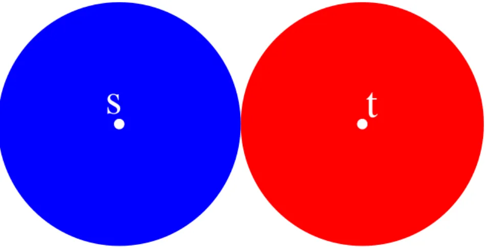
One basic variant of Dijkstra’s algorithm for the point-to-point SPP is bidi-rectional search; instead of building only one shortest path tree rooted at the source nodes, we also build a shortest path tree rooted at the target node t on the reverse graphG. As soon as one node v becomes settled in both searches, we are guaranteed that the concatenation of the shortests → v path found in the forward search and of the shortestv → t path found in the backward search is a shortests → t path. Since we can think of Dijkstra’s algorithm as explor-ing nodes in circles centered ats with increasing radius until t is reached (see Figure 1.1), the bidirectional variant is faster because it explores nodes in two circles centered at boths and t, until the two circles meet (see Figure 1.2); the area within the two circles, which represents the number of explored nodes, will then be smaller than in the unidirectional case, up to a factor of two.
Dijkstra’s algorithm applied to time-dependent FIFO networks has been op-timized in various ways (29; 31). We note here that in the time-dependent sce-nario bidirectional search cannot be applied, since the arrival time at destina-tion node is unknown. We also remark that all speedup techniques based on finding shortest paths in Euclidean graphs (130) cannot be applied either, since the typical arc cost function, the arc travelling time at a certain time of the day, does not yield a Euclidean graph.
1.4.3
Label-correcting algorithm
On a time-dependent graph, we can use a label-correcting algorithm to com-puted∗(s, t) (Section 1.2) instead of d(s, t, τ ) for τ ∈ T ; label-correcting implies
that the label of a node is not fixed even after the node is extracted from the priority queue, in that a node may be reinserted multiple times, unlike Dijk-stra’s algorithm. We refer to (40) for an excellent starting point on the efficient implementation of TDSPP algorithms. We describe here a label-correcting al-gorithm (40) to compute the cost function associated with the shortest path between two nodess, t ∈ V . Such an algorithm can be implemented similarly to Dijkstra’s algorithm, but using arc cost functions instead of arc lengths. The labelℓ(v) of a node v is a scalar for plain Dijkstra’s algorithm, whereas in this case each label is a function of time. In particular, at termination we want ℓ(v) = d∗(s, v). We initialize the algorithm assigning constant functions as
la-bels: ∀τ ∈ T ℓ(s)(τ ) = 0 and ℓ(v)(τ ) = ∞ ∀v ∈ V . At each iteration we ex-tract the nodeu with minimum ℓ(u) from the priority queue, and relax adjacent
1.4 Related Work 25
Figure 1.1: Schematic representation of Dijkstra’s algorithm search
space
s
t
Figure 1.2: Schematic representation of bidirectional Dijkstra’s
s
t
Figure 1.3: Schematic representation of a hierarchical speedup
tech-nique search space
edges: for each(u, v) ∈ A, a temporary label t(v) = ℓ(u)⊕c(u, v) is created. Then ift(v)(τ ) ≥ ℓ(v)(τ ) for all τ ∈ T does not hold, the arc (u, v) yields an improve-ment for at least one time instant. Hence, we updateℓ(v) = min{ℓ(v), t(v)}. The algorithm can be stopped as soon as we extract a nodeu such that ℓ(u) ≥ ℓ(t). An interesting observation from (40) is that the running time of this algorithm depends on the complexity of the cost functions associated with arcs.
1.4.4
Hierarchical speedup techniques for static road
networks
Many hierarchical speedup techniques have been developed for the SPP on static graphs. The main idea is to preconstruct a graph hierarchy where each level is smaller then the previous one, i.e. it has fewer nodes; shortest paths queries start at the bottom level and are then carried out exploring the hier-archy levels in ascending order, so that most of the search is carried out on the topmost level. Since the number of nodes at each level shrinks rapidly as we progress upwards into the hierarchy, the total number of explored nodes is considerably smaller than in a plain appplication of Dijkstra’s algorithm (see Figure 1.3). Due to the inherent bidirectional nature of these algorithms, these approaches only work on static graphs.
1.4.4.1 Highway Hierarchies
The Highway Hierarchies algorithm (HH) (129; 124; 125) is a fast, hierarchy-based shortest paths algorithm which works on static directed graphs. HH is specially suited to efficiently finding shortest paths in large-scale networks, and
1.4 Related Work 27
has been the first algorithm to report average query times of a few milliseconds on continental sized road networks.
A set of shortest paths is canonical if, for any shortest path p in the set, p = (u1, . . . , ui, . . . , uj, . . . , uk), the canonical shortest path between uiandujis a
subpath ofp. Dijkstra’s algorithm can easily be modified to output a canonical shortest paths tree (129).
The HH algorithm works in two stages: a time-consuming pre-processing stage to be carried out only once, and a fast query stage to be executed at each shortest path request. LetG0 = G. During the first stage, a highway hierarchy
is constructed, where each hierarchy levelGl, for1 ≤ l ≤ L, is a modified
sub-graph of the previous level sub-graphGl−1 such that no canonical shortest path in
Gl−1 lies entirely outside the current level for all sufficiently distant path
end-points: this ensures that all queries between far endpoints on level l − 1 are mostly carried out on level l, which is smaller, thus speeding up the search. Each shortest path query is executed by a multi-level bidirectional Dijkstra al-gorithm: two searches are started from the source and from the destination, and the query is completed shortly after the search scopes have met; at no time do the search scopes decrease hierarchical level. Intuitively, path optimality is due to the fact that by hierarchy construction there exist no canonical short-est path of the form (a1, . . . , ai, . . . , aj, . . . , ak, . . .), where ai, aj, ak ∈ A and the
search level ofaj is lower than the level of bothai, ak; besides, each arc’s search
level is always lower or equal to that arc’s maximum level, which is computed during the hierarchy construction phase and is equal to the maximum levell such that the arc belongs toGl. The speed of the query is due to the fact that
the search scopes occur mostly on a high hierarchy level, with fewer arcs and nodes than in the original graph. A heuristic extension of the HH algorithm to dynamic static graphs with a detailed experimental evaluation can be found in (109).
Hierarchy construction. As the construction of the highway hierarchy is the most complicated part of HH algorithm, and also the most interesting to gain insight on how the algorithm works, we endeavour to explain its main traits in more detail. For simplicity, in this paragraph we will assume that the graph is undirected; therefore, we will denote the set of edges by E. An extension to directed graphs is easy to derive (125; 109). Given a local extensionality param-eterH (which measures the degree at which shortest path queries are satisfied without stepping up hierarchical levels) and the maximum number of hierar-chy levelsL, the iterative method to build the next highway level l + 1 starting from a given level graphGlis as follows:
1. For each v ∈ V , build the neighbourhood Nl
H(v) of all vertices reached
fromv with a simple Dijkstra search in the l-th level graph up to and in-cluding the H-st settled vertex. This defines the local extensionality of
each vertex, i.e. the extent to which the query “stays on levell”. 2. For eachv ∈ V :
(a) Build a partial shortest path tree B(v) from v, assigning a status to each vertex. The initial status forv is “active”. The vertex status is in-herited from the parent vertex whenever a vertex is reached or settled. A vertexw which is settled on the shortest path (v, u, . . . , w) (where v 6= u 6= w) becomes “passive” if
|Nl
H(u) ∩ N l
H(w)| ≤ 1. (1.1)
The partial shortest path tree is complete when there are no more active reached but unsettled vertices left.
(b) From each leaft of B(v), iterate backwards along the branch from t tov: all arcs (u, w) such that u 6∈ Nl
H(t) and w 6∈ NHl (v), as well as their
adjacent verticesu, w, are raised to the next hierarchy level l + 1. 3. Select a set of bypassable nodes on level l + 1; intuitively, these nodes
have low degree, so that the benefit of skipping them during a search out-weights the drawbacks (i.e., the fact that we have to add shortcuts to pre-serve the algorithm’s correctness). Specifically, for a given setBl+1 ⊂ Vl+1
of bypassable nodes, we define the setSl+1of shortcut edges that bypass
the nodes inBl+1: for each pathp = (s, b
1, b2, . . . , bk, t) with s, t ∈ Vl+1 \
Bl+1 and b
i ∈ Bl+1, 1 ≤ i ≤ k, the set Sl+1 contains an edge (s, t) with
c(s, t) = c(p). The core Gl+1C = (VCl+1, ECl+1) of level l + 1 is defined as: VCl+1= Vl+1\ Bl+1,ECl+1 = (El+1∩ (VCl+1× VCl+1)) ∪ Sl+1.
The result of the contraction is the contracted highway network Gl+1C , which
can be used as input for the following iteration of the construction procedure. It is worth noting that higher level graphs may be disconnected even though the original graph is connected.
1.4.4.2 Dynamic Node Routing
Separator-based multi-level methods for the SPP have been used by many au-thors; we refer to (81) for the basic variant. The main idea behind separator-based methods is to define, given a subset of the vertex setV′ ⊂ V , the shortest
path overlay graphG′ = (V′, A′) with the property that A′ is a minimal set of
edges such that ∀u, v ∈ V′ the shortest path length between u and v in G′ is
equal to the shortest path length betweenu and v in G. In other words, there is an arc(u, v) ∈ A′ if and only if for any shortest path fromu to v in G then no
internal node of the paths (i.e. all nodes exceptu and v) belongs to V′. It can be
shown thatG′ is unique (81). Usually, the set of separator nodesV′ is chosen in
1.4 Related Work 29
of similar size. In a bidirectional query algorithm, the components containing source and target node are wholly searched, but starting from the separator nodes only edges of the overlay graphG′are considered. This approach can be
generalized and applied in a hierarchical way, building several levels of overlay graphs with node setsV = V0 ⊇ V1 ⊇ · · · ⊇ VLso that the following property is
mantained:∀l ≤ L−1, for all node pairs s, t ∈ Vlthe part of the shortest path
be-tweens and t that lies outside the level l components to which s and t belong is entirely included in the levell + 1 overlay graph. As the overlay graphs become smaller with the increasing level in the hierarchy, a shortest path computation becomes faster because most of the search for a long-distances, t path takes place on the highest hierarchy level, and thus fewer nodes are explored. A path on the original graph can then be reconstructed, because each arc at levell has a unique decomposition as levell − 1 arcs.
In (126), an arbitrary subset V′ = V′(V ) of V is considered instead of
sep-arator nodes; in practice, the set is chosen in such a way that it contains the most important nodes, i.e. those that appear “more often” on shortest paths. This yields a smaller set V′, more uniformly distributed over the whole graph,
and thus G′ will be smaller, resulting in a smaller space consumption and a
faster query algorithm. However, since in this caseV \ V′is no longer made of
small isolated components, the query algorithm is not as simple as in canonical separator-based methods. From a theoretical point of view the same principle holds: we might want to explore nodes from source and target until the queue in Dijkstra’s algorithm only contains nodes that are covered byV′ (i.e. there is
at least one nodev ∈ V′on the shortest path from the root to any leaf of the
cur-rent partial shortest path tree), and then switch to the overlay graphG′, or to a
higher level in the overlay graph hierarchy in the case of a multi-level approach. This, however, does not yield good results in practice, because we cannot tell in advance how many nodes we will have to explore until the whole partial short-est path tree is covered byV′. The main challenge is therefore to compute the
set of all covering nodes for the partial shortest path treeT rooted at s as quickly as possible.
Many possible strategies are suggested in (126), including an aggressive vari-ant which stops the search whenever a node inV′ is encountered, and which
yields a superset of the covering nodes. Some other analysed possibilities may require a greater computational effort, while finding the minimal set of cover-ing nodes. Once the set (or a superset) of all covercover-ing nodes for a given level of the overlay graph has been computed, the search can switch to the next level, until the shortest path is found, which is guaranteed to happen at the topmost level. The choice of level node setsV = V0, V1, . . . , VL, whereVi = V′(Vi−1) for
all i > 0, is critical for query times: these nodes should correspond to nodes that appear very often on shortest paths, i.e. road network junctions with high-importance, such as highway access points. The Highway Hierarchies algo-rithm (Section 1.4.4.1) is employed in (126) to choose the node sets.
The main advantage of this approach is that overlay graphs can be com-puted in a very short time because they only require the application of Dijk-stra’s algorithm on limited parts of the graph; besides, if a few arc costs change there is no need to recompute the whole overlay graphs, but only a small part of them — the part which is affected by the change. Certainly, if the changed arc does not belong to the partial shortest path tree of a given node, the con-struction phase from that node need not be repeated. In particular, during the pre-processing phase, we can build for each nodev a list of all nodes that can be affected if the cost of one of the outgoing arcs fromv changes. If these lists are kept in memory, then one knows exactly which parts of the overlay graphs are affected by the change and must be recomputed. The construction phase is repeated only when necessary. After the update step the bidirectional query algorithm correctly computes shortest paths.
1.4.4.3 Contraction Hierarchies
One of the main concepts used in the Highway Hierarchies algorithm (Section 1.4.4.1) is that of contraction: bypassable nodes are selected and then iteratively removed from the input graph, adding shortcuts (i.e. new arcs) in order to pre-serve distances with respect to the original graph. The Contraction Hierarchies algorithm (64) is a speedup technique for Dijkstra’s algorithm on static graphs which is based solely on contraction: all nodes are ordered by some importance criterion, and then a hierarchy is generated by iteratively contracting the least important node. Thus, the query algorithm is extremely simple: a bidirectional Dijkstra search is started, where the forward search from the source only relaxes arcs leading to more important nodes, while the backward search from the des-tination only relaxes arcs coming from more important nodes. The Contraction Hierarchies algorithm is remarkably simple, yet it is very effective, yielding large speedups with respect to Dijkstra’s algorithm and a very small space occupation of the preprocessed data. Indeed, if one is interested only in computing short-est path distances (i.e. the sequence of edges that form the shortshort-est path on the original graph is not needed), then the preprocessed graph occupies less space than the original input (64).
Clearly, the node ordering criterion is the crucial part of the algorithm, as it determines the order in which nodes are contracted and thus the quality of the final hierarchy. (64) analyses several different criteria and their combination. One of the most important factors in computing a node’s importance is the arc difference, i.e. the number of shortcuts that would be created if the node is bypassed minus the number of incoming and outgoing arcs of that node. This quantity has an influence on both the space overhead and query perfor-mance; it is easy to see that nodes with small arc difference are more appealing for contraction, as their removal yields a graph with a smaller number of arcs. Another important factor is uniformity: it seems to be a good idea to contract
1.4 Related Work 31
nodes everywhere in the graph, instead of repeatedly contracting nodes in the same small region. Other tested criteria include estimations of the contraction cost and of query performance. Combinations of several criteria with different weights are possible. Since the contraction of a node may influence the node ordering of neighbouring nodes, three strategies are tested:
1. the priority of adjacent nodes is recomputed after each contraction step, 2. the priority of all nodes is recomputed periodically,
3. the priority of the node chosen for contraction is recomputed before the contraction, so that if its priority increases and the node is no longer the minimum element then it is skipped and reinserted into the priority queue with the new value.
An estension of Contraction Hierarchies to the time-dependent case is de-scribed in (17); the authors report the main ideas, but there are no computa-tional experiments. Therefore, it is difficult to analyse the performance of an approach based on contraction only in practice. Interestingly, the ideas in (17) are similar to those described in Chapter 4 of our work, although they have been developed indipendently. We discuss some of the problems that may have arised during the implementation of time-dependent Contraction Hierarchies in Section 4.4.
1.4.5
Goal-directed search:
A
∗A∗ (80) is an algorithm for goal-directed search which is very similar to
Dijk-stra’s algorithm (Section 1.4.2). The difference between the two algorithms lies in the priority key. ForA∗, the priority key of a nodev is made up of two parts:
the length of the tentative shortest path from the source to v (as in Dijkstra’s algorithm), and an underestimation of the distance to reach the target fromv. Thus, the key of v represents an estimation of the length of the shortest path from s to t passing through v, and nodes are sorted in the priority queue ac-cording to this criterion. The function which estimates the distance between a node and the target is called potential functionπ; the use of π has the effect of giving priority to nodes that are (supposedly) closer to target nodet. If the po-tential function is such thatπ(v) ≤ d(v, t) ∀v ∈ V , where d(v, t) is the distance from v to t, then A∗ always finds shortest paths (80); otherwise, it becomes a
heuristic. A∗ is equivalent to Dijkstra’s algorithm on a graph where arc costs
are the reduced costswπ(u, v) = c(u, v) − π(u) + π(v) (82). From this, it can be
easily seen that ifπ(v) = 0 ∀v ∈ V then A∗ explores exactly the same nodes as
Dijkstra’s algorithm, whereas ifπ(v) = d(v, t) ∀v ∈ V only nodes on the shortest path betweens and t are settled, as arcs on the shortest path have zero reduced cost.A∗is guaranteed no more nodes than Dijkstra’s algorithm. In particular, if