HAL Id: hal-00755395
https://hal.inria.fr/hal-00755395
Submitted on 21 Nov 2012
HAL is a multi-disciplinary open access archive for the deposit and dissemination of sci-entific research documents, whether they are pub-lished or not. The documents may come from teaching and research institutions in France or abroad, or from public or private research centers.
L’archive ouverte pluridisciplinaire HAL, est destinée au dépôt et à la diffusion de documents scientifiques de niveau recherche, publiés ou non, émanant des établissements d’enseignement et de recherche français ou étrangers, des laboratoires publics ou privés.
Enhancing the computation of distributed shortest paths
on real dynamic networks
Gianlorenzo d’Angelo, Mattia d’Emidio, Daniele Frigioni, Daniele Romano
To cite this version:
Gianlorenzo d’Angelo, Mattia d’Emidio, Daniele Frigioni, Daniele Romano. Enhancing the compu-tation of distributed shortest paths on real dynamic networks. 1st Mediterranean Conference on Algorithms, Dec 2012, Ein-Gedi, Israel. pp.148-158, �10.1007/978-3-642-34862-4_11�. �hal-00755395�
Enhancing the computation of distributed
shortest paths on real dynamic networks
⋆Gianlorenzo D’Angelo1, Mattia D’Emidio2, Daniele Frigioni2, and Daniele Romano2
1
MASCOTTE Project INRIA/I3S(CNRS/UNSA) 2004 Route Des Lucioles, 06902 Sophia–Antipolis Cedex, France. gianlorenzo.d [email protected]
2 Department of Electrical and Information Engineering, University of L’Aquila, Via
G. Gronchi, 18, I–67100, L’Aquila, Italy. [email protected], [email protected], [email protected]
Abstract. The problem of finding and updating shortest paths in dis-tributed networks is considered crucial in today’s practical applications. In the recent past, there has been a renewed interest in devising new effi-cient distance-vector algorithms as an attractive alternative to link-state solutions for large-scale Ethernet networks, in which scalability and reli-ability are key issues or the nodes can have limited storage capabilities. In this paper we present Distributed Computation Pruning (DCP), a new technique, which can be combined with every distance-vector routing algorithm based on shortest paths, allowing to reduce the total number of messages sent by that algorithm and its space occupancy per node. To check its effectiveness, we combined DCP with DUAL (Diffuse Update ALgorithm), one of the most popular distance-vector algorithm in the literature, which is part of CISCO’s widely used EIGRP protocol, and with the recently introduced LFR (Loop Free Routing) which has been shown to have good performances on real networks. We give experimental evidence that these combinations lead to a significant gain both in terms of number of messages sent and memory requirements per node.
1 Introduction
The problem of computing and updating shortest paths in a distributed network whose topology dynamically changes over the time is a core functionality of today’s communication networks. This problem has been widely studied in the literature, and the solutions found are classified as distance-vector and link-state.
Distance-vector algorithms require that a node knows the distance from each of its neighbors to every destination and stores them in a
⋆
Support for the IPv4 Routed/24 Topology Dataset is provided by National Science Foundation, US Dept of Homeland Security, WIDE Project, Cisco Systems, and CAIDA.
data structure called routing table; a node uses its own routing table to compute the distance and the next node in the shortest path to each destination. Most of the known distance-vector solutions (see e.g. [?,?,?]) are based on the classical Distributed Bellman-Ford method (DBF), origi-nally introduced in the Arpanet [?], which is still used in real networks and implemented in the RIP protocol [?]. DBF has been shown to converge to the correct distances if the link weights stabilize and all cycles have positive lengths [?]. However, the convergence can be very slow (possibly infinite) due to the well-known looping and count-to-infinity phenomena. Link-state algorithms, as for example the Open Shortest Path First (OSPF) protocol widely used in the Internet [?], require that a node knows the entire network topology, to compute its distance to any desti-nation, usually running the centralized Dijkstra’s algorithm, thus requir-ing quadratic space per node. Link-state algorithms are free of looprequir-ing, however each node needs to receive and store up-to-date information on the entire network topology after a change. This is achieved by broad-casting each change of the network topology to all nodes [?] and by using a centralized algorithm for dynamic shortest paths as for example that in [?].
Related works. In the last years, there has been a renewed interest in devising new efficient light-weight distributed shortest paths solutions for large-scale Ethernet networks (see, e.g., [?,?,?,?,?,?]), where distance-vector algorithms seem to be an attractive alternative to link-state solu-tions when scalability and reliability are key issues or when the memory power of the nodes of the network is limited. Notwithstanding this in-creasing interest, the most important distance vector algorithm is still DUAL (Diffuse Update ALgorithm) [?], which is free of looping and is part of CISCO’s widely used EIGRP protocol, although it requires a quite big space occupancy per node. Another distance vector algorithm, named LFR (Loop Free Routing), has been recently proposed in [?]. Compared with DUAL, LFR has the same theoretical message complexity but it uses an amount of data structures per node which is much smaller than that of DUAL. Moreover, it has been experimentally shown to be very effective in terms of both messages sent and memory requirements per node in some real-world networks.
Recently, in [?] a general strategy named DLP (Distributed Leaf Pruning) has been introduced which can be combined with every distance vector algorithm with the aim of reducing the number of messages sent by that algorithm. In particular, DLP is able to avoid any distributed com-putation involving degree-one nodes. In [?] the effectiveness of DLP has
been confirmed by combining it with DUAL and by running experiments on real-world and artificial instances.
Results of the paper. In this paper, we provide a new technique, named Distributed Computation Pruning (DCP), which is a generaliza-tion of DLP and can be combined with every distance-vector algorithm with the aim of overcoming some of their main limitations in real-world networks (high number of messages sent, high space occupancy per node, low scalability, poor convergence). DCP has been designed to be efficient mainly in networks following a power-law node degree distribution, which from now on will be referred as power-law networks. The main idea un-derlying DCP rely on the fact that a power-law network with n nodes typically has average node degree much smaller than n and a high number of nodes with small degree (less than 3). Nodes with small degree often do not provide any useful information for the distributed computation of shortest paths, that is there are many topological situations in which these nodes should neither perform nor be involved in any kind of dis-tributed computation, as their shortest paths depend on those of higher degree nodes.
In order to check the effectiveness of DCP, we combined it with DUAL and LFR by obtaining two new algorithms named DUAL-DCP and LFR-DCP, respectively. Then, we implemented the two new algo-rithms in the OMNeT++ simulation environment [?], a network simula-tor which is widely used in the literature. We also implemented DUAL, LFR, DUAL-DLP and LFR-DLP, where the last two algorithms are the combination of DUAL and LFR with DLP [?]. As input to the al-gorithms, we considered instances of power-law networks similar to those used in [?] and [?], that is the Internet topologies of the CAIDA IPv4 topology dataset [?] (CAIDA, Cooperative Association for Internet Data Analysis, is an association which provides data and tools for the analysis of the Internet infrastructure) and the random topologies generated by the Barab´asi-Albert algorithm [?].
The results of our experiments can be summarized as follows: the com-bination of DUAL and LFR with DCP provides a huge improvement in the number of messages sent with respect to DUAL and LFR, respec-tively. In particular, on the CAIDA instances, the number of messages sent by DUAL-DCP is always between 3% and 16% that of DUAL, while the number of messages sent by LFR-DCP is always between 10% and 26% that of LFR. The gain is significant also with respect to DUAL-DLP and LFR-DLP. In particular, DUAL-DCP sends a number of messages which is between 11% and 40% that of DUAL-DLP, while
LFR-DCP sends a number of messages which is between 21% and 58% that of LFR-DLP. We observed also an improvement in the maximum space occupancy per node of DUAL-DCP and LFR-DCP, and in the average space occupancy per node of DUAL-DCP. This is due to the fact that nodes with small degree do not need to store some of the data structures implemented by DUAL and LFR, respectively. We obtained similar results also for the Barab´asi-Albert instances.
2 Preliminaries
We consider a network made of processors linked through communication channels that exchange data using a message passing model, in which: each processor can send messages only to its neighbors; messages are delivered to their destination within a finite delay but they might be delivered out of order; there is no shared memory among the nodes; the system is asynchronous, that is, a sender of a message does not wait for the receiver to be ready to receive the message. We are interested in the practical case of networks whose topologies dynamically change over the time due to update operations on the edges (weight increase, weight decrease, insert, delete).
Graph notation. We represent a network by an undirected weighted graph G = (V, E, w), where V is a finite set of n nodes, one for each processor, E is a finite set of m edges, one for each communication chan-nel, and w is a weight function w : E → R+ that assigns to each edge
a real value representing the optimization parameter associated to the corresponding channel. An edge in E that links nodes u, v ∈ V is de-noted as {u, v}. Given v ∈ V , N (v) denotes the set of neighbors of v, and deg(v) = |N (v)| denotes the degree of v. The maximum degree of the nodes in G is denoted by maxdeg. A path P in G between nodes u and v is denoted as P = {u, ..., v}. The weight of P , denoted as w(P ) is the sum of the weights of the edges in P . A shortest path be-tween nodes u and v is a path from u to v with the minimum weight. The distance d(u, v) from u to v is the weight of a shortest path from u to v. Given two nodes u, v ∈ V , the via from u to v is the set of neighbors of u that belong to a shortest path from u to v. Formally: via(u, v) ≡ {z ∈ N (u) | d(u, v) = w(u, z) + d(z, v)}. Given a time t, we denote as wt(), dt(), and viat() the edge weight, the distance, and the via at time t, respectively. We denote a sequence of update operations on the edges of G by C = (c1, c2, ..., ck). Assuming G0 ≡ G, we denote
con-sider the case that operation ci either increases or decreases the weight
of an existing edge in Gi. The extension to delete and insert operations
is straightforward.
Distance-vector algorithms. Given a graph G = (V, E, w), distance-vector routing algorithms based on shortest-paths usually share a set of common features. In detail, a generic node v of G: (i) knows the identity of every other node of G, the identity of all its neighbors and the weights of the edges incident to it; (ii) maintains and updates its own routing ta-ble that has one entry for each s ∈ V , which consists of at least two fields: D[v, s], the estimated distance between v and s, and VIA[v, s], the neighbor used to forward data from v to s; (iii) handles edge weight increases and decreases either by a single procedure (see, e.g., [?]), which we denote as WeightChange, or separately (see, e.g., [?,?]) by two procedures, which we denote as WeightIncrease and WeightDecrease; (iv) asks infor-mation to its neighbors through a message denoted as query, receives replies by them through a message denoted as reply. If the routing infor-mation on a node changes, a distance vector algorithm propagates such a variation as follows:
– if v is performing WeightChange, then it sends to its neighbors a message, from now on denoted as update; a node that receives this kind of message executes a procedure named Update;
– if v is performing WeightIncrease or WeightDecrease, then it sends to its neighbors message increase or decrease, resp.; a node that
receives increase/decrease executes a procedure named Increase/Decrease, respectively.
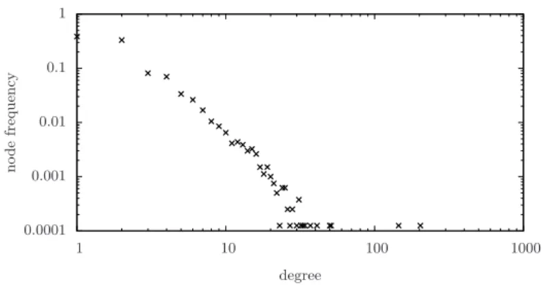
Power-Law networks. Power-law networks are very important in prac-tice and includes many of the currently implemented communication in-frastructures, like the Internet, the World Wide Web, some social net-works, and so on [?]. Practical examples of power-law networks are the Internet topologies of the CAIDA IPv4 topology dataset [?]. The CAIDA dataset is collected by a globally distributed set of monitors. The moni-tors collect data by sending probe messages continuously to destination IP addresses. Destinations are selected randomly from each routed IPv4/24 prefix on the Internet such that a random address in each prefix is probed approximately every 48 hours. The current prefix list includes approxi-mately 7.4 million prefixes. For each destination selected, the path from the source monitor to the destination is collected, in particular, data col-lected for each path probed includes the set of IP addresses of the hops which form the path and the Round Trip Times (RTT) of both
inter-0.0001 0.001 0.01 0.1 1 1 10 100 1000 n o d e fre q u en cy degree
Fig. 1: Power-law node degree distribution of a CAIDA graph with 8000 nodes and 11141 edges
mediate hops and the destination. In Fig. 1 we report the node degree distributions of a CAIDA network.
3 Dynamic scenarios
In this section, we introduce some preliminary definitions that are useful to capture the possible dynamic scenarios typical of power-law networks and we show some properties of shortest paths in these scenarios. Given an undirected weighted graph G = (V, E, w), we classify the nodes of G with respect to their degree as follows. A node v ∈ V is:
– central if deg(v) ≥ 3:
– peripheral if deg(v) = 1;
– semiperipheral if deg(v) = 2. An edge {u, v} of G is:
– central if both u and v are central;
– peripheral if either u or v is peripheral;
– semiperipheral if either u or v is semiperipheral and neither of them is peripheral.
A path P = {v0, v1, ..., vj−1} in G is:
– central if it is made only of central edges;
– peripheral if it contains exactly one peripheral edge and exactly one central node; the unique central node of P is called owner of P ;
c4 sp1 j u c1 c2 c3 sp3 sp2 p1 p2 p3 v
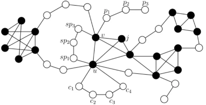
Fig. 2: A graph G and its corresponding nodes classification.
– semiperipheral if it is formed only by semiperipheral edges. If v0 and
vj−1 are two distinct central nodes, then they are called semiowners
of P . If v0 ≡ vj−1, then P is a semiperipheral cycle, and v0 ≡ vj−1 is
called the cycleowner of P .
In Fig. 2 we report an example of a graph G and its nodes classifi-cation. Central nodes are drawn in black while the non-central ones are drawn in white. The path {u, j, v} is a central path, the path {v, p1, p2, p3}
is a peripheral path whose owner is v, the path {u, sp1, sp2, sp3, v} is
a semiperipheral path whose semiowners are u and v, while the path {u, c1, c2, c3, c4, u} is a semiperipheral cycle whose cycleowner is u.
The following lemmata introduce some basic relationships between central and non-central shortest paths of the network.
Lemma 1 (Peripheral shortest paths). Given a graph G = (V, E, w), let P = {v, p1, ..., pj−1} be a peripheral path of G whose owner is node v,
and let P′ = {v, p1, ..., pi}, 1 ≤ i ≤ j − 1, be a sub-path of P containing
v. Then, for each x ∈ V \ {p1, ..., pj−1}, d(x, pi) = d(x, v) + w(P′).
Proof. Let us assume, by contradiction, that d(x, pi) 6= d(x, v) + w(P′).
Then, two cases may arise: d(x, pi) > d(x, v)+w(P′) or d(x, pi) < d(x, v)+
w(P′). In the first case, it follows that d(x, pi) is not a distance, which is a
contradiction. In the second case, it follows that there must exist at least two different paths with different weights from x to pi, which is again a
contradiction as pi belongs to a peripheral path and P′ is the shortest
path between v and pi in G. ⊓⊔
Lemma 2 (Semi-peripheral shortest paths). Given a graph G =
semiowners are nodes u and v, and let S′ = {u, sp
1, ..., spi}, 1 ≤ i ≤
j − 2, and S′′ = {spi, ..., spj−2, v} be two sub-paths of S, containing u
and v, respectively. Then, for each x ∈ V \ {sp1, ..., spj−2}, d(x, spi) =
min{d(x, u) + w(S′), d(x, v) + w(S′′)}.
Proof. By contradiction, assume that d(x, spi) 6= min{d(x, u)+w(S′), d(x, v)+
w(S′′)}. Two cases may occur: d(x, spi) > min{d(x, u) + w(S′), d(x, v) +
w(S′′)} or d(x, sp
i) < min{d(x, u) + w(S′), d(x, v) + w(S′′)}. In the first
case, it follows that d(x, spi) is not a distance, which is a contradiction.
In the second case, it follows that there must exist a third different path from x to spi, with different weight, which is a contradiction, as spi is a
semiperipheral node. ⊓⊔
Lemma 3 (Semi-peripheral cycle shortest paths). Given a graph
G = (V, E, w), let C = {u, c1, ..., cj−1, u} be a semiperipheral cycle of
G whose cycleowner is node u, and let C′ = {u, c1, ..., ci} and C′′ =
{ci, ..., cj−1, u}, 1 ≤ i ≤ j − 1, be two sub-paths of C. Then, for each
x∈ V \ {c1, ..., cj−1}, d(x, ci) = min{d(x, u) + w(C′), d(x, u) + w(C′′)}.
Proof. The proof is similar to that of Lemma 2 ⊓⊔
Some useful additional relationships can be derived introducing time instants in the above Lemmata. In particular, by Lemma 1 we know that, if between the time instants ti and ti+1 the weight of the edge {p1, p2}
be-tween two nodes belonging to a peripheral path P = {v, ..., p1, p2, ..., pj−1}
changes, that is wti(p
1, p2) 6= wti+1(p1, p2), then for each x ∈ V that does
not belong to P , the distance from p1 to x does not change, while the
distance from p2 to x changes as follows:
dti+1(p
2, x) = dti(p2, x) + wti+1(p1, p2) − wti(p1, p2) (1)
By Lemma 2 we know that, if between the time instants ti and ti+1the
weight of the edge {sp1, sp2} between two nodes belonging to a
semipe-ripheral path S = {u, ..., sp1, sp2, ..., v} changes, that is wti(sp1, sp2) 6=
wti+1(sp
1, sp2), then for each x ∈ V , both the distances from sp1to x and
from sp2 to x change as follows:
dti+1(sp 1, x) = min z∈N (sp1) {dti+1(z, x) + wti+1(sp 1, z)} (2) dti+1(sp 2, x) = min z∈N (sp2) {dti+1(z, x) + wti+1(sp 2, z)} (3)
Let us assume that, between ti and ti+1, the weight of the edge
{u, ..., c0, c1, c2, c3, ..., u} changes, that is wti(c1, c2) 6= wti+1(c1, c2). If
we denote as C0 = (u, ..., c0, c1), C1 = (c1, c2, ..., u), C2(u, ..., c1, c2) and
C3 = (c2, c3, ..., u) then by Lemma 3, for each x ∈ V , the distances from
c1 to x and from c2 to x change as follows:
dti+1(c 1, x) = dti(x, u) + min{ X {l,q}∈C0 wti+1(l, q), X {l,q}∈C1 wti+1(l, q)} (4) dti+1(c 2, x) = dti(x, u) + min{ X {l,q}∈C2 wti+1(l, q), X {l,q}∈C3 wti+1(l, q)} (5)
If the distance between a generic node x ∈ V and a central node c changes between the time instants ti and ti+1 (that is, dti+1(x, c) 6=
dti(x, c)), then the following relationships hold:
– by Lemma 1, for each peripheral path P = {c, ..., p, ..., pj−1} with
owner c, and for each p ∈ P : dti+1(x, p) = dti
(x, p) + dti+1(x, c) − dti
(x, c), (6)
– by Lemma 2, for each semiperipheral path S = {c, ..., sp, ..., d} with semiowners c and d and for each sp ∈ S such that c belongs to the shortest path from sp to x at time ti, if we denote as D = (d, ..., sp)
the sub-path of S from d to sp), then:
dti+1(x, sp) = min{dti+1(x, sp) + dti+1(x, c) − dti
(x, c) , dti
(x, d) + X
{l,q}∈D
wti
(l, q)}(7)
– by Lemma 3, for each cyclic path C = {c, c1, ..., c, ..., cj−1, c} with
cycleowner c, and for each c ∈ C: dti+1(x, c) = dti
(x, c) + dti+1(x, c) − dti
(x, c), (8)
4 The new technique
Distributed Computation Pruning (DCP) has been designed to be effi-cient mainly in power-law networks, by forcing the distributed computa-tion to be carried out only by the central nodes, which are few in prac-tice. The non-central nodes, which are the great majority in power-law networks, receive updates about routing information passively from the respective owners, without starting any kind of distributed computation. Then, the larger is the set of non-central nodes of the network, the bigger
is the improvement in the pruning of the distributed computation and, consequently, in the global number of messages sent.
Data structures. Given a generic distance-vector algorithm A, DCP requires that a generic node of G stores some additional information with respect to those required by A. In particular, a node v needs to store and update information about non-central paths of G. To this aim, v maintains a data structure called ChainP ath, denoted as CHPv, which is
an array containing one entry CHPv[s], for each central node s. CHPv[s]
stores the list of all edges, with the corresponding weight, belonging to the non-central paths containing s.
A central node is obviously not present in any list of CHPv. A
pe-ripheral node is present in exactly one list CHPv[s], where s ∈ V is its
owner. A semi-peripheral node is present in exactly two lists CHPv[v0] and
CHPv[vj−1], if it belongs to a semi-peripheral path (v0 and vj−1 are its semi-owners), while it is present in a single list CHPv[v0], if it belongs to a
semi-peripheral cycle (v0 is its cycle-owner). The space occupancy
over-head per node due to ChainP ath can be quantified using the following observations:
– the ChainP ath contains at most as many entries as the number of the central nodes;
– the sum of the sizes of all the lists in the ChainP ath is twice the number of non-central edges of G in the worst case;
– the number of non-central edges of G is O(n), as they belong to paths in which every node has degree at most two.
Hence, the space overhead per node due to CHPv is O(n). Note that,
despite the overhead due to the ChainP ath data structure, the use of DCPcan induce a decrease in the space occupancy per node required by A for the following observations: (i) in most of the cases nodes do not ask and do not need to store information received from non-central nodes; (ii) computations which involves the whole network are performed only with respect to central destinations. In Section 5 we will experimentally confirm this behavior.
Distributed Computation Pruning. The combination of DCP with a distance vector algorithm A induces a new algorithm denoted as A-DCP. The behavior of A-DCP can be summarized as follows. While in a classic routing algorithm every node performs the same code thus having the same behavior, in A-DCP central and non-central nodes have different behaviors. In particular, central nodes detect changes concerning all kind
of edges, while semiperipheral, peripheral and cyclic nodes detect changes concerning only semiperipheral, peripheral and cyclic edges, respectively. If the weight of a central edge {u, v} changes, then node u (v, resp.) performs the procedure provided by A for the distributed computation of the shortest paths, only with respect to central nodes. During this compu-tation, if u (v) needs information by its neighbors, it asks only to central neighbors or, if u (v) is the semiowner of one or more semiperipheral paths, it asks information also to the other semiowner of each semipe-ripheral path, by means of a strategy we called Mod-DBF. In detail, node u (v) sends to each semiperipheral neighbor a queryDBF message, whose aim is to traverse the semiperipheral path, in order to get infor-mation by the other semiowner. The queryDBF message contains just one field, the source object of the computation. A semiperipheral node, which receives a queryDBF message from one of its two neighbors, sim-ply performs a store-and-forward step and sends a queryDBF message to the other neighbor. A central node, which receives a queryDBF message, simply replies the information that queryDBF is asking for. Once u (v) has updated its own routing information, it propagates the variation to all its neighbors through the update, increase or decrease messages of A. When a generic node x receives an update, increase or decrease message, it stores the current value of D[x, s] in a temporary variable.
Now, if x is a central node, then it handles the change and updates its routing information toward s, by using the proper procedure of A (Update, Increase, or Decrease) and propagates the new informa-tion to its neighbors. Otherwise, if x is a peripheral, semiperipheral or cyclic node, it handles the change and updates its routing information toward s by using Lemmata 1–3, and the data provided by its owner, semiowner and cycleowner, respectively. At the end, x verifies whether the routing table entry of s is changed or not and, in the affermative case, it updates the routing information about the non-central neighbors of s, if they exist, by implementing Equations 6–8. Note that, node x uses the data contained in CHP in order to properly update its routing information towards the non-central nodes of s, if they exist.
If a weight change occurs on a peripheral edge {u, v}, then nodes u and v both send a p change(u, v, w(u, v)) message to each of their neigh-bors. When a generic node x receives message p change, it first verifies whether the update has been already processed or not, by comparing the new value of w(u, v) with the one stored in its CHP. In the first case the message is discarded. Otherwise, node x updates its CHP with the updated value of w(u, v) and its routing information by using Equation 1. Then,
it propagates the change by a flooding algorithm to forward the message over the network.
If the weight of a semiperipheral edge {u, v} changes, then node u (v resp.) sends two kind of messages: a sp change(u, v, w(u, v)), to each of its owners, and a sp update(s, D[u, s]) (sp update(s, D[v, s])) to v (u), for each s such that VIA[u, s] 6= v (VIA[v, s] 6= u). When a generic node x receives message sp change, it first verifies whether the update has been already processed or not, by comparing the new value of w(u, v) with the one stored in its CHP. In the first case the message is discarded. Otherwise, node x simply updates its CHP with the updated value of w(u, v). When a generic node x receives a sp update(s, D[u, s]) message from a neighbor u, two cases can occur. If x is a central node, it simply performs procedure update of A. Otherwise, it updates routing information towards s by using Equations 2–3. Note that, in this case, node x uses the information contained in CHP in order to verify whether it belongs or not to the same semiperipheral path of s and to properly update its routing information. If the weight of a cyclic edge {u, v} changes, nodes u and v both send a cy update(u, v, w(u, v)) message to each of their neighbors. When a generic node x receives message cy update, it first verifies whether the update has been already processed or not, by comparing the new value of w(u, v) with the one stored in its CHP. In the first case the message is discarded. Otherwise, node x updates its CHP with the updated value of w(u, v) and its routing information by using Equations 4–5. Then, it propagates the change by a flooding algorithm to forward the message over the network.
5 Experimental analysis
In this section we report the results of our experimental study on DUAL, LFR, DUAL-DLP, LFR-DLP, DUAL-DCP and LFR-DCP. Our ex-periments have been performed on a workstation equipped with a Quad-core 3.60 GHz Intel Xeon X5687 processor, with 12MB of internal cache and 24 GB of main memory, and consist of simulations within the OM-NeT++ 4.0p1 environment [?]. The programs have been compiled with GNU g++ compiler 4.4.3 under Linux (Kernel 2.6.32).
Executed tests. For the experiments we used the power-law networks of the CAIDA IPv4 topology dataset [?]. We parsed the files provided by CAIDA to obtain a weighted undirected graph, denoted as GIP, where a
node represents an IP address in the dataset (both source/destination hosts and intermediate hops), edges represent links among hops and
weights are given by Round Trip Times. As the graph GIP consists of
almost 35000 nodes, we could not use it for the experiments, as the amount of memory required to store the routing tables of all the nodes is O(n2· maxdeg) for DUAL. Hence, we performed our tests on connected
subgraphs of GIP, with a variable number of nodes and edges, induced
by the settled nodes of a breadth first search starting from a node taken at random. We denoted a h nodes subgraph of GIP with GIP−h. We
gen-erated a set of different tests, each test consists of a subgraph of GIP
and a set of k edge updates, where k assumes values in {5, 10, . . . , 200}. An edge update consists of multiplying the weight of a random selected edge by a percentage value randomly chosen in [50%, 150%]. For each test configuration (a graph with a fixed value of k) we performed 5 differ-ent experimdiffer-ents (for a total amount of 200 runs) and we report average values.
Analysis. We ran simulations on CAIDA instances with different num-ber of nodes n ∈ {1200, 5000, 8000}. The results of our experiments on the different instances are similar, hence we report those on the bigger instances, which has 8000 nodes and 11141 edges.
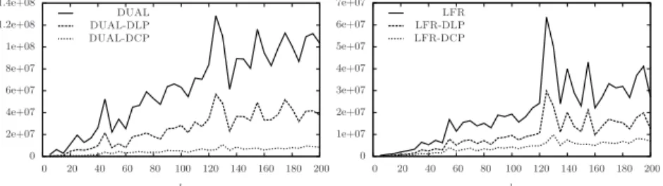
In particular, in Figures 3(left) and 3(right) we report the number of messages sent by DUAL, DUAL-DLP and DUAL-DCP and by LFR, LFR-DLP and LFR-DCP, respectively, on GIP−8000. Notice that, GIP−8000 has average node degree equal to 2.8, a percentage of degree 1 nodes ap-proximately equal to 38.5%, and a percentage of degree 2 nodes approxi-mately equal to 33%. The figures show that the combinations of DUAL and LFR with DCP provide a huge improvement in the global number of messages sent. The gain is significant also with respect to DUAL-DLP and LFR-DLP. In the tests of Fig. 3(left) the ratio between the number of messages sent by DUAL-DCP and DUAL is within 0.03 and 0.16 which means that DUAL-DCP sends a number of messages which is between 3% and 16% that of DUAL. Similarly, the ratio between the number of messages sent by DUAL-DCP and DUAL-DLP is within 0.11 and 0.40. In the tests of Fig. 3(right) the ratio between the number of messages sent by LFR-DCP and LFR is within 0.10 and 0.26 which means that the number of messages sent by LFR-DCP is always between 10% and 26% that of LFR. Similarly, the ratio between the number of messages sent by LFR-DCP and LFR-DLP is within 0.21 and 0.58.
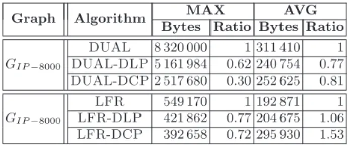
To conclude our analysis, we consider the space occupancy per node of each algorithm. The results are summarized in Table 1 where we report the maximum and the average space occupancy per node, in Bytes, of each algorithm on GIP−8000. We also report the ratio between the space
0 2e+07 4e+07 6e+07 8e+07 1e+08 1.2e+08 1.4e+08 0 20 40 60 80 100 120 140 160 180 200 k DUAL DUAL-DLP DUAL-DCP 0 1e+07 2e+07 3e+07 4e+07 5e+07 6e+07 7e+07 0 20 40 60 80 100 120 140 160 180 200 k LFR LFR-DLP LFR-DCP
Fig. 3: Number of messages sent by DUAL, DLP and DUAL-DCP(left) and by LFR, LFR-DLP and LFR-DCP (right) on GIP−8000.
occupancy per node of the algorithms integrating DLP and DCP and that of the original algorithms, for each test instance. Note that, since the space occupancy per node of LFR, LFR-DLP and LFR-DCP depends on the number of weight change operations, we show median values for each of these algorithms.
Our experiments show that the use of DCP induces, in most of the cases, a clear improvement also in the space requirements per node. In par-ticular, DUAL-DCP (LFR-DCP) requires a maximum space occupancy per node which is 0.30 (0.72) and 0.29 (0.83) times that of DUAL (LFR)
in GIP−8000 and GBA−8000, respectively. Notice that, the improvement is
more evident in the case of DUAL, as its maximum space occupancy per node is by far higher than that of LFR. Concerning DUAL, this be-havior is confirmed also in the average case, where DUAL-DCP requires 0.81 and 0.92 times the average space occupancy per node of DUAL, in
GIP−8000and GBA−8000, respectively. On the contrary, our data show that
the average space occupancy per node of LFR-DCP is slightly greater than that of LFR and that the use of DCP induces an overhead in the average space occupancy per node which is equal to 53% and 77%, in
GIP−8000 and GBA−8000, respectively. This is due to the fact that the
av-erage space occupancy of LFR is quite low by itself and that, in this case, the space occupancy overhead needed to store the ChainP ath is greater than the space occupancy reduction induced by the use of DCP. As a final remark, notice that, the use of DCP represents an improvement in the maximum space occupancy per node also with respect to the use of DLP(See Table 1).
Graph Algorithm MAX AVG Bytes Ratio Bytes Ratio GI P−8000 DUAL 8 320 000 1 311 410 1 DUAL-DLP 5 161 984 0.62 240 754 0.77 DUAL-DCP 2 517 680 0.30 252 625 0.81 GI P −8000 LFR 549 170 1 192 871 1 LFR-DLP 421 862 0.77 204 675 1.06 LFR-DCP 392 658 0.72 295 930 1.53
Table 1: Space occupancy per node of the implemented algorithms.
References
1. R. Albert and A.-L. Barab´asi. Emergence of scaling in random networks. Science, 286:509–512, 1999.
2. D. Bertsekas and R. Gallager. Data Networks. Prentice Hall International, 1992.
3. S. Cicerone, G. D’Angelo, G. Di Stefano, and D. Frigioni. Partially dynamic ef-ficient algorithms for distributed shortest paths. Theoretical Computer Science, 411:1013–1037, 2010.
4. S. Cicerone, G. D’Angelo, G. Di Stefano, D. Frigioni, and V. Maurizio. Engineering a new algorithm for distributed shortest paths on dynamic networks. Algorithmica, to appear, DOI: 10.1007/s00453-012-9623-9, 2012.
5. S. Cicerone, G. D. Stefano, D. Frigioni, and U. Nanni. A fully dynamic algorithm for distributed shortest paths. Theoretical Computer Science, 297(1-3):83–102, 2003.
6. G. D’Angelo, M. D’Emidio, D. Frigioni, and V. Maurizio. A speed-up technique for distributed shortest paths computation. In ICCSA 2011, volume 6783 of LNCS, pages 578–593, 2011.
7. G. D’Angelo, M. D’Emidio, D. Frigioni, and V. Maurizio. Engineering a new loop-free shortest paths routing algorithm. In SEA 2012, volume 7276 of LNCS, pages 123–134, 2012.
8. D. Frigioni, A. Marchetti-Spaccamela, and U. Nanni. Fully dynamic algorithms for maintaining shortest paths trees. Journal of Algorithms, 34(2):251–281, 2000.
9. J. J. Garcia-Lunes-Aceves. Loop-free routing using diffusing computations.
IEEE/ACM Trans. on Networking, 1(1):130–141, 1993.
10. P. A. Humblet. Another adaptive distributed shortest path algorithm. IEEE Trans.
on Communications, 39(6):995–1002, Apr. 1991.
11. Y. Hyun, B. Huffaker, D. Andersen, E. Aben, C. Shannon, M. Luckie,
and K. Claffy. The CAIDA IPv4 routed/24 topology dataset.
http://www.caida.org/data/active/ipv4 routed 24 topology dataset.xml.
12. J. McQuillan. Adaptive routing algorithms for distributed computer networks. Technical Report BBN Report 2831, Cambridge, MA, 1974.
13. J. T. Moy. OSPF: Anatomy of an Internet routing protocol. Addison-Wesley, 1998.
14. A. Myers, E. Ng, and H. Zhang. Rethinking the service model: Scaling ethernet to a million nodes. In ACM SIGCOMM HotNets. ACM Press, 2004.
15. OMNeT++. Discrete event simulation environment. http://www.omnetpp.org.
16. S. Ray, R. Gu´erin, K.-W. Kwong, and R. Sofia. Always acyclic distributed path computation. IEEE/ACM Trans. on Networking, 18(1):307–319, 2010.
17. E. C. Rosen. The updating protocol of arpanet’s new routing algorithm. Computer
Networks, 4:11–19, 1980.
18. N. Yao, E. Gao, Y. Qin, and H. Zhang. Rd: Reducing message overhead in DUAL. In Proceedings 1st International Conference on Network Infrastructure and Digital
Content (IC-NIDC09), pages 270–274. IEEE Press, 2009.
19. C. Zhao, Y. Liu, and K. Liu. A more efficient diffusing update algorithm for loop-free routing. In 5th International Conference on Wireless Communications,