On the non-convergence of energy intensities: Evidence from a pair-wise econometric approach

(1)

13, allée François Mitterrand BP 13633 49100 ANGERS Cedex 01 Tél. : +33 (0) 2 41 96 21 06 Web : http://www.univ‐angers.fr/granem

On the non‐convergence of energy

intensities: evidence from a pair‐wise

econometric approach

Yannick Le Pen

LEMNA (Université de Nantes)

Benoît Sévi

GRANEM (Université d’Angers) et LEMNA (Université de Nantes)

Décembre 2008

Document de travail du GRANEM n° 2008‐08‐008

(2)

Document de travail du GRANEM n° 2008‐08‐008

décembre 2008

Classification JEL : C32, O40, Q43, Q50.

Mots‐clés : Intensité énergétique, test par paire, test de racine unitaire, ruptures structurelles, convergence.

Keywords: Energy intensity, pair‐wise test, unit‐root test, stationarity test, structural break, convergence.

Résumé : Ce papier examine la convergence des intensités énergétiques pour un groupe de 97 pays sur la

période 1971‐2003. La notion de convergence est testée en utilisant une méthode récemment proposée par

Pesaran (2007) [M.H. Pesaran. A pair‐wise approach to testing for output and growth convergence. Journal of

Econometrics 138, 312‐355.] qui se base sur le critère de convergence stochastique. Les principaux avantages

de cette méthode sont que les résultats ne dépendent pas d’une variable référence face à laquelle la

convergence est testée, et qu’elle est plus robuste. L’application de plusieurs tests de racine unitaire et d’un

test de stationnarité rejette l’hypothèse de convergence. Localement, pour les sous‐groupes Moyen‐Orient,

OCDE et Europe, la non convergence est moins fortement rejetée. L’introduction d’éventuelles ruptures

structurelles dans l’analyse apporte un soutien à peine supérieur à l’hypothèse de convergence.

Abstract: This paper evaluates convergence of energy intensities for a group of 97 countries in the period

1971‐2003. Convergence is tested using a recent method proposed by Pesaran (2007) [M.H. Pesaran. A pair‐

wise approach to testing for output and growth convergence. Journal of Econometrics 138, 312‐355.] based on

the stochastic convergence criterion. Main advantages of this method are that results do not depend on a

benchmark against which convergence is assessed, and that it is more robust. Applications of several unit‐root

tests as well as a stationarity test uniformly reject the global convergence hypothesis. Locally, for Middle‐East,

OECD and Europe sub‐groups, non‐convergence is less strongly rejected. The introduction of possible

structural breaks in the analysis only marginally provides more support to the convergence hypothesis.

Yannick Le Pen

Institut d’Economie et de Management de Nantes – IAE

Université de Nantes

yannick.le‐pen@univ‐nantes.fr

Benoît Sévi

Faculté de Droit, Economie et Gestion

Université d’Angers

benoit.sevi@gmail.com

© 2008 by Yannick Le Pen and Benoît Sévi. All rights reserved. Short sections of text, not to exceed two paragraphs, may be quoted without explicit permission provided that full credit, including © notice, is given to the source. © 2008 by Yannick Le Pen et Benoît Sévi. Tous droits réservés. De courtes parties du texte, n’excédant pas deux paragraphes, peuvent être citées sans la permission des auteurs, à condition que la source soit citée.

(3)

Yannick Le Pen

2

Universit´

e de Nantes (LEMNA)

Benoˆıt S´

evi

3

Universit´

e d’Angers (GRANEM) and LEMNA

December 2008

Abstract: This paper evaluates convergence of energy intensities for a group of 97 countries in the period 1971-2003. Convergence is tested using a recent method proposed by Pesaran (2007) [M.H. Pesaran. A pair-wise approach to testing for output and growth convergence. Journal of Econometrics 138, 312-355.] based on the stochastic convergence criterion. Main advantages of this method are that results do not depend on a benchmark against which convergence is assessed, and that it is more robust. Applications of several unit-root tests as well as a stationarity test uniformly reject the global convergence hypothesis. Locally, for Middle-East, OECD and Europe sub-groups, non-convergence is less strongly rejected. The introduction of possible structural breaks in the analysis only marginally provides more support to the convergence hypothesis.

JEL Classification: C32, O40, Q43, Q50.

Keywords: Energy intensity, pair-wise test, unit-root test, stationarity test, structural break, convergence.

1_{Acknowledgments to be added.}

2_{Address for correspondence: Institut d’´}_{Economie et de Management de Nantes – IAE, Universit´e de Nantes, Chemin de}

la Censive du Tertre, BP 52231, 44322 Nantes cedex 3. Email address: yannick.le-pen@univ-nantes.fr

3_{Faculté de Droit, ´}_{Economie et Gestion, Université d’Angers, 13 allée Fran¸cois Mitterrand, BP 13633, 49036 Angers}

(4)

1 Introduction

This paper evaluates the relevance of the energy intensities convergence hypothesis for an international data set of 97 countries for the period 1971-2003 by applying a new convergence criterion . This topic is of importance, in particular given the on-going debate on economic growth and its relationship with energy consumption for developing countries. It is also related to the issue of climate change because energy consumption is known to be by far the most pollutant gas emitting activity.

In addition, concerns about climate change, the scarcity of fossil fuels and their recent associated high and volatile prices have reopened the issue of energy intensity dynamics. Besides, Ang and Liu (2006) recently showed that energy intensity has moved from an increasing to a decreasing trend thereby motivating an analysis of the dynamics, if any, of the convergence process. Beyond the analysis of changes in the structure of energy consumption4 _{arises the question of the relative levels of energy} intensities between countries. When this issue is dynamically investigated, the convergence debate is then entered into.

The convergence of energy intensities has received little attention in comparison with convergence of other energy-related variables such as carbon intensities or emission levels of pollutants.5 _Even if energy consumption and energy productivity play a major role in the determination of carbon intensity, they also bear some extra information. Energy intensity measures a direct link between energy consumption and economic activity. The relation between emission levels and the economy, while of primary concern for environmental policy, is less direct (Ang, 1999). Therefore, a better understanding of the spatial distribution of energy intensities and an investigation of the convergence of this variable may lead to new insights. The hypothesis of convergence between national energy intensities, despite its neglect in the literature, is of crucial importance for a number of reasons. First and foremost, it may help to establish fair environmental constraints, which allows developing countries to maintain or increase their growth and developed countries to sustain a sufficient level of consumption. Indeed, the design of coherent policies aiming at fulfilling international protocol targets such as the Kyoto protocol depends on both the levels and the distribution of energy intensities among countries. The determination of caps for emission permits markets should be less influenced by historical levels than by the revealed patterns of convergence. Kolstad (2005, p. 2231), speaking about emission targets, notes that “cost uncertainty can be reduced through the use of intensity reduction targets.” This is because intensity reduction targets can be adapted to the rate of growth of GDP compared to the total amount of emissions. In the same vein, Markandya et al. (2006) suggest that an objective of non-increasing consumption may be reached for developing countries if their growth remains limited with regard to the convergence towards efficiency process.

Second, a lack of convergence could reveal a specific pattern in the diffusion of energy-related technolo-gies. A better knowledge of this diffusion could guide regulatory incentives and technological policies aiming at encouraging knowledge diffusion.

Third, forecasting energy intensity is of primary importance for public or private energy decision

4_{Energy consumption decomposition is by far the most treated issue in the energy economic literature. Recent examples}

are Sue Wing (2008) who analyses the decrease in the US energy intensity at the industry level and Fisher-Vanden et al. (2004) who consider China’s energy intensity decline using firm-level data.

5_{Nevertheless, as coined by Romero- ´}_{Avila (2008, p. 2268) when speaking about emissions convergence: “A related issue}

(5)

makers in order to manage networks, as well as storage capacities and other economic or industrial structures. Again, the knowledge of patterns of energy use and the dynamics of this factor may help to forecast required investment, at least for energy distributed through networks.

Fourth, energy intensities convergence has significant implications for policy decision-makers in terms of fairness in the fight against climate change. As noted by Sun (2002, p. 631): “An aim in human development and progress is not only development and progress in parts of countries and/or regions, but a decrease in the imbalance between countries and/or regions”. This, of course, both concerns energy consumption and energy intensity.6 _{But, as pointed out in McKibbin and Stegman (2005)} and Barassi et al. (2008), the concept of fairness is questionable owing to the strong path-dependent nature of energy intensity. Indeed, energy intensity is strongly related to natural resources in each country and the historical of countries.7

Fifth, the knowledge of a convergence process also provides some insights into the differential impacts of energy industrial sector liberalization. In this respect the study by Markandya et al. (2006) leads to an implicit examination of the liberalization process now occurring in developed and transition countries. It may be of interest to analyze the impact of liberalization on the technology diffusion process as well as on the resulting change in the energy intensity ratio.

Finally, the analysis of convergence of energy intensities could contribute to the debate on the existence of an Environmental Kuznets Curve (EKC).8 _{If convergence occurs then the conclusion drawn by} Dasgupta et al. (2002) that “Since these societies [developing countries] are nowhere near the income range associated with maximum pollution on the conventional environmental Kuznets curve, a literal interpretation of the curve would imply substantial increases in pollution during the next few decades” (p. 148, brackets from the authors) are reinforced. Likewise, evidence of convergence in addition to population pressure in developing countries, give more weight to conclusions from Ang and Liu (2006) that “The aggregate energy intensity of an industrial country would be about three times that of a low income developing countries in 1975, but it would only be half of that of the latter in 1997. It appears that while the high income countries have been able to achieve significant reductions in the growth of energy consumption for each percentage growth of economic growth, the growth in energy consumption has remained high as compared to economic growth in the low income countries.” (p. 2403) The strong relationship between emissions and energy consumption means that the inverted U-shaped relationship largely posited in the literature between pollution and economic development may also be highlighted with data using energy intensities instead of emissions.9

Until now, to our knowledge, the convergence of energy intensities has been described by rather de-scriptive methods. Nilsson (1993) analyzes 31 countries (a mix of developed and developing countries) over the period 1950 to 1988. A graphical analysis suggests a convergence process for most of the countries in the full sample. Convergence occurs towards a level between 0.25 and 0.5 tonne of oil equivalent per 1000 (1980) international dollars, well below the level observed in developed economies

6_{The recent proposal entitled “Contraction and Convergence” from the Global Commons Institute presented in}

Romero-´

Avila (2008) aims at equating emissions in a global reduction framework. It should affect energy intensity as well.

7_{It is common knowledge that energy intensity suffers from a strong inertia, rendering constraints dedicated to modify}

energy consumption sometimes very costly for some industries and people working in these industries.

8_{See Dasgupta et al. (2002) and Stern (2004) for recent surveys and Lindmark (2002, 2004) for an historical perspective}

with respect to carbon intensities.

9_{Sun (1999) goes one step further on the relation between energy and emissions by advocating the existence of an EKC}

(6)

over recent years (at the time of writing). Of course, the absence of statistical tests for convergence is an argument for the use of a conclusive method. Alcantara and Duro (2004) resort to the Theil Index to measure dispersion within and between groups but their results are still descriptive and not validated by the mean of a statistical measure. It then appears that a statistical analysis may be fruitful to shed more light on the issue of convergence of energy intensities. All the more so since no theoretical model provides predictions about this question. In the particular case of transition countries, Markandya et al. (2006) argue that the observed income convergence would be a grounds for energy intensities convergence, a kind of “economy convergence” as a whole.10 _{It is tempting to} verify these predictions empirically.

In our paper, we test whether national energy intensities are converging over time or not. We use a data set of 97 countries over the period 1971-2003. Our methodology is drawn from Pesaran (2007). It is based on the stochastic convergence criterion provided in Bernard and Durlauf (1995) in the context of per capita income convergence. Stochastic convergence between two variables is said to occur if their differential is a stationary process around a constant.11 _{In this case, the observed divergences between} these variables are only a temporary phenomenon and are expected to disappear in the future. The application of a unit-root or a stationarity test to the differentials under study was the natural way to test for convergence. Evidence of unit-root was a sufficient condition to reject convergence. Panel data unit-root or stationarity tests gave the possibility to test for convergence for several countries at the same time. However, a drawback of these panel tests is that a benchmark is always necessary and that the answer is not always clear. For instance, they do not give us the extent of the convergence process, if it exists.

Pesaran (2007) proposes an alternative way to use results from unit-root and stationarity tests to investigate convergence. The main idea is to consider all possible pairs of countries and apply to each pair a selected test on the differential. It is then possible to compute the number of stationary differentials and to compare it with the total number of pairs. In case of convergence, the ratio of the non trending stationary differential is expected to be close to 100%.12 _{A main advantage of the method} is that it is benchmark-free, while a possible disadvantage appears to be the difficulty of finding a case of convergence given the imposed criterion (see discussion in section 3.3).

It has been well known since Perron (1989) that ignoring structural breaks in the analysis of unit-root may lead to an under-rejection of the unit-root hypothesis. Because Pesaran’s analysis of convergence is built on a given unit-root or stationarity tests, this method is also subject to this criticism. We decided to apply Pesaran’s methodology with tests allowing for breaks in order to take into account the possibilities of structural change and their potential impacts on the convergence hypothesis. The outline of the paper is as follows. The following section presents some background literature, spe-cific to the energy-variables convergence issue. Section 3 sets out the pairwise approach and discusses some drawbacks of alternative methods and of the method itself. In section 4 we present our data and the empirical results given by the application of some unit-root and stationarity tests. In section 5, we allow for one structural break in the deterministic component and test whether this hypothesis

10_{Note that such predictions, justifiable at the regional level, cannot be easily extended to a larger sample of countries}

where initial conditions, industrial structures, natural resources and political and regulatory environments are extremely diversified today, as well as in the past.

11_{See also Bernard and Durlauf (1996) for an interpretation of the results of their 1995’s paper and Islam (2003) for a}

discussion of methodologies. Pesaran proposes a weaker stochastic convergence criterion.

(7)

increases the share of stationary differentials. Finally section 6 provides some concluding remarks and possible extensions to the present work.

2 Related literature

Different methods, drawn from the literature on economic growth, have been employed to assess convergence in energy-related variables. Although an exhaustive presentation of these methods is beyond the scope of this paper, it seems appropriate, at least for a better understanding of the advantages of Pesaran’s (2007) methodology, to present some of them.13 _{In the present section, we} survey these methods with reference not only to energy intensity but also to carbon intensity and GHG emissions convergence.

First of all, the almost standard σ14 _{and β convergence}15 _{criteria (see Sala-i-Martin, 1996) have been} applied to the analysis of energy-related variables. Sun (2002) computed mean deviation within groups of countries and between groups of countries in order to show that the differences in energy intensities between OECD countries decreased from 1971 to 1998. This kind of analysis is similar in nature to

σ-convergence.16 _{Miketa and Mulder (2005) and Mulder and De Groot (2007) rely on β-convergence,} conditional β-convergence and σ-convergence to investigate energy productivity convergence at the industry level.17 _{Miketa and Mulder (2005) use a panel of 56 countries for the period 1971-1995} and focus on the within convergence as well as on the convergence speed in each industrial sector. Mulder and De Groot (2007) use a smaller sample of countries but with more detailed data on the same period. The authors provide evidence of the “catch-up” hypothesis and local rather than global convergence. Markandya et al. (2006) also rely on β-convergence to investigate the convergence of energy intensity in 12 transition countries of Eastern Europe towards energy intensity levels in countries from the EU15. Empirical results show some evidence of convergence towards the EU average despite significant differences in the rate of convergence appearing.18

Quah (1993, 1996a and b) stresses the failure of the aforementioned σ and β-convergence criteria. He argues that these criteria are not discriminating enough and can therefore lead us conclude erroneously in favor of convergence, for instance in cases of overtaking. He therefore advocates the investigation of the dynamics of the distribution of the variables. This approach has been followed by Ezcurra (2007b) who analyzes the spatial distribution of energy intensities in 98 countries over the period 1971-2001. Patterns of convergence seem evident from his analysis and the estimated ergodic (limiting) distri-bution provides evidence of a single-peaked future. Ezcurra (2007b) also highlights a limited degree

13_{We focus here only on references in energy economics. References from the growth literature are generally not mentioned}

here but can be found for instance in the survey by Islam (2003).

14_{The σ-convergence criterion is accepted if a measure of the dispersion of distribution of the variable of interest decreases}

over time.

15_{In that case, we check if the growth rate of the variable of interest is negatively correlated to its initial level (unconditional}

convergence) given extra regressors (conditional convergence).

16_{Alcantara and Duro (2004) extend Sun’s (2002) analysis by employing the Theil index used for instance in industrial}

economics to measure concentration in industries as well as in development economics to measure inequalities. Empirical evidence indicates a contribution of both within and between-group to the global fall in energy intensity.

17_{Resorting to industry level data allows to put forward some patterns sometimes dissimulated in aggregate data. In this}

respect, both of these papers are particulary relevant because they permit to explain why convergence or divergence may be achieved or not at the aggregate level.

18_{An analysis of the energy intensity of transition countries is provided in Cornillie and Fankhauser (2004) giving some}

(8)

of intra-distribution mobility19 _{thus leading to a slow dynamic towards the single mode distribution.} The same methodology has been applied by Nguyen Van (2005) for the analysis of carbon dioxide emissions convergence in 100 countries for the period 1966-1996. In this case, conclusions are less clear-cut (see also Ezcurra, 2007a). Convergence seems to be confirmed for developed countries but not for the full sample including developing countries. Aldy (2007) also relies on Quah’s (1993, 1996a and b) methodology to investigate the convergence of carbon dioxide emissions at the State level in the US and provide evidence of divergence. Finally, Stegman and McKibbin (2005) investigate the issue of convergence for a range of energy-related variables with a particular focus on per capita carbon emissions. These authors do not conclude in favor of convergence for the full cross section but do when the sample is restricted to OECD countries.

As stated in the introduction, stochastic convergence is another way to test for convergence. In this case, we are interested in the dynamic properties of the series. According to Bernard and Durlauf’s (1995) definition, convergence between two energy intensities is accepted if their differential is a zero-mean stationary process, which implies that it doesn’t contain a unit-root nor a deterministic trend. Pesaran slightly relaxes this criterion and proposes to accept convergence if the differential is a station-ary process around a constant. If this condition is accepted, we expect that the differential will reach its mean value in the future. Another way to interpret this criterion is that the possible deterministic and stochastic trends which rule the dynamics of each energy intensities are the same. The literature on stochastic convergence has evolved as new unit-root and stationary tests emerged from time se-ries econometrics. Panel data unit-root tests such as the one in Im et al. (2003) are one interesting development in this field. Their higher power, compared with standard univariate unit-root tests, have made those panel unit-root tests particularly attractive. To our knowledge, these tests have not yet been applied to the energy intensity convergence issue.20 _{Nevertheless, they have been used in} related studies such as the carbon dioxide emissions convergence (Strazicich and List (2003), Aldy (2006), Barassi et al. (2008) and Westerlund and Basher (2008))21_{, the causality between income and} emissions (Dinda and Coondoo, 2006) and air pollutant emissions (Bulte et al., 2007). Romero- ´Avila (2008) is in the same vein and resorts to the recent econometric techniques developed in Carrion-i-Silvestre et al. (2005) to investigate convergence when multiple breaks in the series are possible. The issue of breaks in the series is also investigated in Westerlund and Basher (2008) using Lanne and Liski’s (2004) methodology and Chang and Lee (2008).22

The innovative way to deal with the convergence proposed in Pesaran (2007) and applied in Pesaran

et al. (in press) also relies on stochastic convergence. However, standard unit-root tests, as well as

panel data unit-root tests, impose the choice of a benchmark, such as a country or a mean, against which to test for convergence. The results of the tests depends on the choice of this benchmark which, of course, weakens their robustness. In order to reach a higher degree of certainty, Pesaran proposes

19_{This can be deduced from an examination of the diagonal coefficients of the estimated stochastic matrix. If these}

coefficients are close to 1, the probability to move along the distribution is low and the distribution tends to remain quite unchanged.

20_{An exception which uses unit-root panel tests along with energy data is Lee (2005) whose aim is to investigate causality}

between energy consumption and GDP in 18 developing countries. This is a quite different question that the one we analyze in the present paper.

21_{The study by Westerlund and Basher (2008) is an interesting extension of papers by Strazicich and List (2003) and Aldy}

(2006). It uses very recent panel unit-root tests allowing for cross-sectional dependence (Phillips and Sul (2003), Bai and Ng (2004) and Moon and Perron (2004)), a critical assumption for carbon dioxide emissions data because independence is very unlikely to hold in this case. Nevertheless, Westerlund and Basher (2008) do not examine significance of the deterministic trend, and as noted in the introduction, their method is not immune to the choice of a benchmark.

(9)

considering all possible pairs of energy intensities and applying a unit-root or a stationarity test to each of their differentials.23

Thus, our motivation for the present analysis and for the use of this tool is to rely on a robust benchmark-free method in order to investigate the issue of energy intensities convergence. This is not the case for all previous methodologies presented above. In the next section, we present the pairwise approach developed in Pesaran (2007) which will be used in conjunction with either a stationarity or a unit-root test.

3 Econometric methodology: the pairwise approach

Pesaran’s (2007) pairwise convergence approach24 _{is based on the stochastic convergence criterion of} Bernard and Durlauf (1995). Let’s denote eitand ejtcountries i and j energy intensity, respectively, at time t and dij,t= eit− ejt, t = 1, ..., T (where T denotes the number of observations) their differential. These energy intensities are said to be convergent in the Bernard and Durlauf’s view if their differential is an I(0) process around a constant. Under the convergence hypothesis, Hc, we can then write :

Hc : deij,t= eit− ejt= cij+ ψij,t

for all i 6= j where ψij,t is a zero mean stationary process.

In Bernard and Durlauf’s paper, the mean differential cij is set to zero. Pesaran allows this parameter not to be null and shows that this condition means that the differentials are bounded from above in the long term. Both criteria imply that these energy intensities share the same deterministic and stochastic trends. If each energy intensity contains a unit-root, this criterion is satisfied if there is a cointegrating vector [1,-1] between them. This latter condition is called the cointegration condition. However, the cointegration condition is necessary but not sufficient. Another condition is that both energy efficiencies share the same deterministic trend if they have one. This condition is called the

cotrending condition. When both the cointegration and the cotrending conditions are satisfied, the

energy intensities differential will converge to its expectation in the future and discrepancies from this value would only be transitory.

A problem with the implementation of stochastic convergence is that usual unit-root and cointegration tests cannot handle a large number of countries at the same time. Researchers usually bypass this difficulty by using a benchmark country either, real or virtual (by means of an average calculation as in, for instance, Romero- ´Avila (2008)) against which convergence is tested. However, results heavily depend on this benchmark. Pesaran’s approach sets round this issue by considering all possible pairs of countries. If our sample contains N countries, we will test convergence for the N (N − 1)/2 possible pairs of energy efficiency differentials. Another feature of Pesaran’s method is that the fraction of differentials which are characterized as stationary around a constant will provide evidence on the validity of the convergence hypothesis as previously mentioned. In addition, Pesaran et al. (in press)

23_{Another contribution related to energy markets also considers convergence issue relying on a pairwise approach:}

Zach-mann (2008). The author makes use of pairwise convergence in a more intuitive Zach-manner and does not rely on any statistical test as will be the case in Pesaran.

24_{In Pesaran, it is applied to the longstanding issue of output and growth convergence. It is also employed in Pesaran et}

(10)

note that “the average rejection rate is likely to be more robust to the possibility of an I(1) unobserved factor, inducing cross-section dependence, than the alternative methods available.” (p. 5)

Besides the fact that the Pesaran’s method is benchmark-free, it is also very flexible in the sense that every parametric, semi-parametric or nonparametric unit-root or stationarity test can be used in conjunction with this approach. In the present study, because our empirical work is not derived from any theoretical model, we do not favor unit-root or stationarity tests, and resort to both.25 _One drawback of Pesaran’s methodology is that we lose the interesting analysis of the speed of convergence (see for instance Westerlund and Basher (2008) for developments on this issue). This is the price to pay for a more robust answer to our main research question, namely energy intensities convergence. We now give more details on the methodology when applied, first, with a stationarity test and then with a unit-root test.

3.1 Stationarity tests

Kwiatkowski et al. (1992) KPSS stationarity test around a constant can be used to test convergence. In this case, we can see that the null hypothesis of stationarity around a constant is similar to the convergence hypothesis Hc. When we reject this null hypothesis, we reject convergence. We apply this stationarity test to each of the N (N − 1)/2 energy intensity differentials and define the binary variable Zij,T which is equal to 1 if we reject the null hypothesis of stationarity and 0 otherwise. We note α the size of the stationarity test defined as the probability of rejecting the null hypothesis of stationarity even if convergence is true that is to say: limT →∞P (Zij,T = 1 | Hc) = α. The fraction of the N (N − 1)/2 pairs for which the convergence hypothesis is rejected is given by:

¯ ZN T = 2 N (N − 1) N −1_X i=1 N X j=i+1 Zij,T

Pesaran shows that, under the null hypothesis of convergence Hc, ¯ZN T is a consistent estimator of α for a large N and T , that is :

lim

T →∞E( ¯ZN T | Hc) = α

Therefore, if the hypothesis of convergence is true, we may sometimes reject the stationary hypothesis but this rejection rate is expected to converge to the level of the test. A rejection rate ¯ZN T well above the chosen level of the test means that the rejection of convergence cannot be explained by type-I error but really comes from a lack of convergence.26 _{We can notice here one difference between this} method and a panel data unit-root test. Panel data unit-root tests are based on the computation of the average of each statistical test while Pesaran approach is based on the average of a binary variable

25_{In contrast, when the hypothesis to be tested derives from a strong assumption as it is the case for the PPP hypothesis}

for instance, then the null hypothesis should conform with this assumption (the stationarity of the price differential here, see Bai and Ng (2004)). Hence, Romero- ´Avila (2008) advocates to consider first the stationarity hypothesis, which is not motivated in the case of carbon dioxide convergence examination.

26_{Pesaran shows that under H}

c, the expected value of ¯ZN T goes to α as T → ∞ and the variance goes to zero as N

increases even if some Zij,Tand Zik,T are not independent as they represent overlapping pairs of countries which share

(11)

which describes the result of each individual test. This difference in methodologies may sometimes lead to quite different conclusions.

3.2 Unit-root tests

Another way to proceed is to apply a unit-root test to each of the energy intensities differentials deijt. With unit-root test, the null hypothesis becomes divergence, denoted ¯Hc. Note that divergence may arise because the differential contains a unit-root, or a deterministic trend or both. We therefore apply a unit-root test with a deterministic trend to each energy intensity differential and define Zij,T = 1 if the unit-root hypothesis is rejected and Zij,T = 0 otherwise. In that case, ¯ZN T estimates the fraction of differentials for which the null hypothesis of a unit-root with a trend is rejected. If the hypothesis of energy efficiency convergence Hcis true, ¯ZN T is expected to be much greater than the size α of the unit-root test and to converge to unity as N → ∞ and T → ∞ jointly.

If the hypothesis of no convergence ¯Hc is true, ¯ZN T is expected to be close to α. In this latter case, rejection of the unit-root hypothesis merely reflects the occurrence of type -I error in the test. Each of the unit-root tests is run with an intercept and a linear trend. If the unit-root hypothesis is rejected, we test for the significance of the linear trend with a Student test.

We expect that the stationarity test will supply more favorable results to the convergence scenario when comparing unit-root with stationarity tests. Indeed, in the case of stationarity test, the null is the stationarity hypothesis and, as such, the favored hypothesis.

3.3 General discussion of the methodology

As discussed above, Pesaran’s methodology relies on the stochastic convergence approach developed in Bernard and Durlauf (1995). We have mentioned that results supplied by Pesaran’s approach should be more robust than those provided by previous applications of unit-root or stationarity tests for at least two reasons. First, in previous empirical exercises, results are sensitive to the choice of a benchmark against which convergence has to be tested. Second, Pesaran gives more precise information on the rejection or acceptation of an hypothesis given the presence of the type-I error. Indeed, with a large set of regressions, if the number of rejections is near the level of the test, then the null hypothesis can be accepted due to the knowledge of the type-I error existence. A last advantage of Pesaran’s method is that it is not based on the modelling of an alleged average behavior of an average energy intensity differential. Each differential is modelled separately and has its own dynamics. These are major advantages when investigating the convergence hypothesis.

In his paper, Pesaran indicates that in case of convergence, the percentage of stationary differentials should be close to 100%. However, in practice, convergence may be defined in a weaker sense. For instance, the stationarity of a large proportion of differentials may be an indicator of convergence. The remaining conclusion being that Pesaran’s method seems to have more ability to compare levels of convergence between groups than to discriminate between convergence and non-convergence in a given sample.

Finally, a problem appears because of the stochastic convergence criterion itself. Namely, convergence is reached if the unit-root hypothesis is rejected. Perhaps this criterion imposes a too strong condition

(12)

on the data. Results in Pesaran provide weak support for the output convergence hypothesis for the second part of the 20th century, even among developed countries. They confirm previous findings of Bernard and Durlauf (1995). Several authors have tried to amend this approach in order to obtain conclusions less unfavorable to the convergence hypothesis. A first possibility was to use more powerful tests, such as panel data unit-root tests. Another one, proposed by Oxley and Greasley (1995) was to modify the convergence criterion by taking into account the possibility of a structural break. This break is supposed to model the dynamics of countries who are converging but have not reached their long-run dynamics. Bernard and Durlauf (1996) showed that the application of a unit-root test without structural break was unable to detect such a dynamic. In this paper we follow this last approach and take into account structural breaks.

4 Data and analysis without break

4.1 Data

Our data cover a sample of 97 countries for the time period 1971-2003 (see appendix). Data on energy use per capita (kt of oil equivalent) are extracted from the World Development Indicators (2007). Data on real per capita GDP are taken from the PWT 6.2 (Heston et al., 2006). Per capita GDP are expressed in international dollars in year 2000 constant price and converted with a PPP rate. Energy intensity is defined as the ratio of energy use per capita to per capita GDP. The first sample we consider is made up of the 97 countries for which we could find a complete set of data. This sample allows us to check if convergence in energy intensities is a global phenomenon. However, convergence could be limited to some narrower sets of countries, usually called “convergence clubs”. We therefore consider different sub-groups of countries selected on the basis of economic as well as geographical criteria. This exogenous composition of country groups is, of course, subject to the criticism of being biased in favor or not of convergence. However, the endogenization of convergence clubs is beyond the scope of this paper.27

4.2 Preliminary graphical analysis

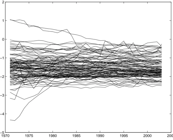
We begin our empirical analysis by a plot of the data in order to get a feeling of the possible convergence phenomenon. As in Romero- Ávila (2008) and Westerlund and Basher (2008) for carbon dioxide emissions levels, we plot in figure 1 the log of energy intensities relative to their cross sectional means for each date. Despite Pesaran’s method being benchmark-free, plotting variables relative to their cross sectional means may be of interest for detecting patterns of convergence. Visual inspection of the resulting graph does not deliver clear evidence of convergence, even if the gap between the lowest and the highest energy intensities has decreased during the period. Their trajectories toward the bulk of energy intensities appears to be marginal. In contrast with Romero- Ávila (2008) and Westerlund and Basher (2008), no clear pattern emerges from this graph. It could be argued that the sample is not long enough but the period is the same as in, for instance, Romero- Ávila (2008). A first conclusion that might be drawn from this figure is that energy intensities are relatively stable over time, perhaps due to its established inertia (see McKibbin and Stegman, 2005). The next conclusion is that a statistical

(13)

analysis is necessary to determine whether or not patterns of convergence exist in the data.

4.3 Empirical results

We begin with the presentation of results given by several unit-root tests and go on to the results from the application of the KPSS stationarity test. We use the three following unit-root tests: the Augmented Dickey-Fuller (ADF) unit-root test, the ADF-GLS unit-root test (Elliot et al., 1996), and the ADF-WS unit-root test (Park and Fuller, 1995) as in the original articles of Pesaran (2007) and Pesaran et al. (in press). These are commonly employed tests in unit-root literature and do not seem to suffer from major drawbacks in comparison with more computer intensive tests such as the ones of semi or nonparametric class. We include an intercept and a deterministic trend in each ADF regression and choose the number of lagged difference terms according to three information criteria, namely the Akaike criterion (AIC), the Schwarz criterion (SC) and the Hannan-Quinn criterion (HQ).

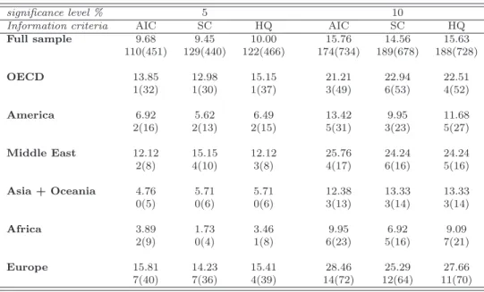
Results for the ADF unit-root test for the full sample as well as for sub-groups are summarized in table 1. This table reports the proportions of the differentials for which the unit-root hypothesis is rejected at a 5% and a 10% significance level for each information criterion. The full sample consists in 97 countries or 4656 pairs which appears to be sufficient enough to consider N as large. Considering results for the sample of 97 countries, they are not in favor of convergence for two reasons. Firstly, the rejection rates of the null unit-root hypothesis are only slightly superior to the nominal level of the test. For instance, when the level of the test is set to 5%, the rejection rates fluctuate between 9.45% (with AIC) and 10% (with HQ). This difference cannot be easily considered as significant. Secondly, when we consider the energy intensities for which we are able to reject the null unit-root hypothesis, the deterministic trend appears to be insignificant in roughly 25% of these cases.28 _For instance, when we run the ADF test with a 5% level and the AIC criterion, we are able to accept an insignificant trend for 54 of the 243 pairs for which we reject the unit-root hypothesis. These results therefore stand against the convergence hypothesis. Results are more contrasted when we consider the different sub-groups. Rejection rates of the null unit-root hypothesis are clearly above the level of the test for the OECD, the Middle East and Europe. When the level of the test is set to 5%, these rates fluctuate between the minimum of 12.12% (for Middle-East with AIC and HQ) and the maximum of 15.81% (Europe with AIC). These rejection rates cannot be attributed to the type-I error and denotes an absence of stochastic trend in these energy differentials. However when we consider the other condition of convergence, that is to say the absence of a deterministic trend, one can see that condition is hardly satisfied. For instance, in the case of the OECD countries, the number of insignificant trend is equal to 1 among the number of stationary differentials which varies between 30 and 37. We can draw the same conclusion for the Middle-East and Europe. For America, Asia and Oceania, and Africa groups, rejection rates are of the same order as the level of the test, indicating that rejections may be the product of the type-I error. It must be noted that for the Middle East and Asia and Oceania groups, with 12 and 15 countries respectively, results have to be regarded with caution. In these cases, the “N large” assumption is of course subject to caution.

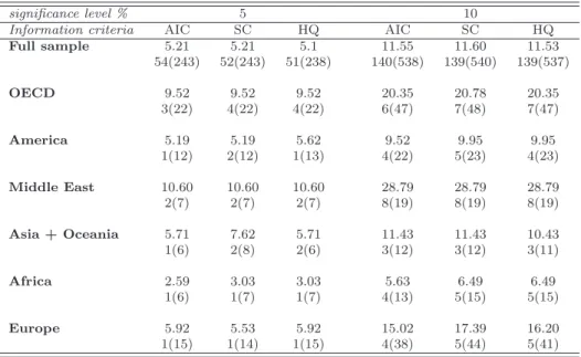
Results from the Elliot et al.’s (1996) ADF-GLS unit-root test with an intercept and a deterministic trend are reported in table 2. For each group, as well as for the full sample, rejection rates decrease.

(14)

This does not change qualitatively the results of the ADF test, but may highlight that the ADF-GLS test is perhaps more conservative. Overall, the convergence hypothesis remains strongly rejected. The Europe group now exhibits less evidence of weak convergence in comparison with the ADF test. Conversely, the Middle-East and OECD groups remain groups where convergence rejection is less evident than in other cases.

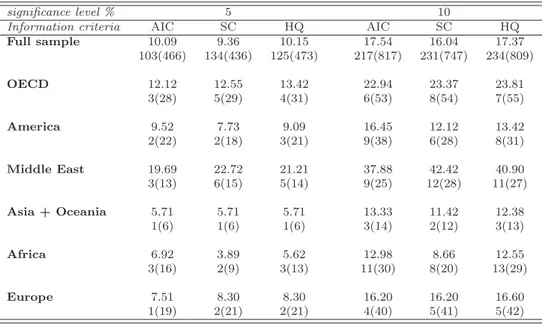
We finally apply Park and Fuller’s (1995) ADF-WS unit-root test, which is known as being more powerful than the two others.29 _{Results for the ADF-WS test are reported in table 3. Rejection rates} are higher than for the other tests. Nevertheless, the proportion of differentials for which the unit-root hypothesis is rejected remains low in all cases except for the Middle-East.30 _{In addition, the number} of stationary differentials with an insignificant deterministic linear trend is still very low, which stands against the convergence hypothesis.

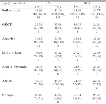
We now apply the KPSS test for which stationarity is the null hypothesis. 31 _{Results are reported} in table 4. For the ease of comprehension, results are presented as the proportion of non-rejection of the stationarity hypothesis. This proportion is expected to be near 100% in cases of convergence occurring and close to the level of the test if there is no convergence. Apart the case of the Middle East countries and Africa, the estimated rates of non-rejection are quite sensitive to the level of the stationarity test or the lag truncation parameter. When we run a 5% level stationarity test, the rates of non-rejection are above this level for each groups, which indicates some evidence of convergence. However, when we run a 10% level stationarity test, these rates of non-rejection decreases and become much closer to 10%, particularly when the lag truncation parameter is set to 1. The only group for which the rate of non-rejection remains greater than 10% is the Middle-East, which confirms previous results from the ADF test.

Our results of the unit-root and stationarity tests without structural break can be summarized as follows. Convergence is uniformly rejected for all groups, including the full sample. Nevertheless, results can be marginally discussed for the Middle-East, Europe and OECD, for which the evidence of non-convergence is a bit less clear. Despite the discussion of Pesaran’s methodology in the previous section, our results provide conclusions in sharp contrast with papers such as Sun (2002), Alcantara and Duro (2004), Markandya et al. (2006) and Ezcurra (2007b). Moreover, we find very weak evidence of regional convergence, which is found in Miketa and Mulder (2005).32 _{The lack of global and regional} convergence may be supported by the very disparate initial endowment in terms of natural resources which heavily conditions national energy intensities.

A possible extension of the present analysis would be to resort to Sieve bootstrap (see B¨uhlman, 1997) as proposed in Pesaran et al. (in press) to increase the precision of the estimate of the share of stationary differentials. Sieve bootstrap is suited for time series because it conserves a dependence structure similar to the one initially present in the data. We did not opt for this option because our results come out against convergence with little uncertainty.

29_{Leybourne et al. (2005) have recently noted that ADF-WS has good size and power properties compared to other tests.} 30_{Again, it should be noted that the low number of countries in this group leads to conclude with care about this group.} 31_{The lag window is set to l ≈ 0.75T}1/3_{as it is currently done in the time series literature}

32_{Miketa and Mulder (2005) cite Keller (2002) “technology diffusion and knowledge spillovers are local rather than global.”}

(15)

5 Pairwise approach with one structural break

A natural question that emerges when considering series over a long enough time period is the possi-bility of structural breaks in the deterministic component. In our case, the hypothesis of a structural break must be considered for two reasons. Firstly, Perron’s (1989) seminal contribution has shown that a unmodeled structural break could lead to an under rejection of the unit-root hypothesis. However, Perron’s testing strategy was criticized because the break date was chosen on a a priori basis and not endogenously. Several authors proposed to extend Perron’s approach in order to select the break date endogenously. Among these papers, Zivot and Andrews (1992) modified the ADF unit-root test while the more recent Kurozumi (2002) stationarity test with a structural break is based on the KPSS test. The other reason to consider the possibility of a structural break is directly linked to the field of energy economics. Findings from Nilsson (1993), indicating a decoupling of energy consumption and growth after 1973, could also indicate some changes in energy systems. As noted in section 2, breaks have also been considered in the analysis of energy-related series by Lanne and Liski (2004), Romero- ´Avila (2008), Westerlund and Basher (2008) and Chang and Lee (2008). Beyond the fact that all these contributions have an interest in the analysis of carbon dioxide emissions, while we study energy intensities, another difference has to be noted. We investigate convergence in a benchmark-free framework, whereas these studies33_{are all, because of the methodology used, benchmark-dependent.} Pesaran’s methodology can be used in conjunction with a test allowing for breaks without notable difficulty. We apply the pairwise approach with the Zivot and Andrews (1992) and the Kurozumi (2002) tests. Our aim is to check if the introduction of a structural break in our test will increase the rejection rate of the unit-root test with the Zivot and Andrews unit-root test or the rate of non-rejection of the stationarity hypothesis with the Kurozumi stationarity test, thus providing evidence of convergence. Several authors such as Oxley and Greasley (1995) have already applied unit-root tests with structural breaks to test the convergence hypothesis in the growth literature.

Even if the hypothesis of a structural break in the deterministic component does not exactly match our initial convergence criterion, we think that this hypothesis deserves to be investigated. First, the absence of a unit-root has a consequence on the forecasting of the future values of energy differentials. Second, some kind of structural changes can accord with our definition of convergence, for instance if there is only a change in the intercept and no deterministic trend, or if the slope of the deterministic trend becomes insignificant in the second part of the sample. Given the limited number of observations for each series, we assume that only a single break can occur during the time period spanned by the data.

5.1 Stationarity test with one structural break

We first apply Kurozumi’s (2002) stationarity test with a change in the intercept. As with the KPSS test, the variable Zij,T is now equal to 1 if we reject the null hypothesis of stationarity with a structural break and 0 otherwise. The ratio

(16)

is therefore the rejection rate of the null hypothesis of stationarity. We expect this ratio to be close to the size of the test if the convergence hypothesis is the true hypothesis. To check for the presence of a structural break, we apply the Supf and the Expf tests of Andrews (1996) and Bai and Perron (1996, 2003) to each series for which the null hypothesis of stationarity is accepted. If this structural break is confirmed, we test whether the intercept is significant after the break date.

5.2 Unit-root test with one structural break

We apply Zivot and Andrews (1992) unit-root test with a change in the coefficient of the deterministic linear trend, that is to say the changing growth model. This choice can be discussed. However, we think that a change in the slope of the trend is a more realistic representation of the behavior of the energy intensity differential for the time period considered. As above, we define the dichotomic variable Zij,T which is equal to 1 if we reject the unit-root null hypothesis with a structural break and 0 otherwise. The ratio

is therefore the rejection rate of the null unit-root hypothesis and we expect it to be close to 100% if convergence really occurs. For each energy intensities differential for which we can reject the unit-root hypothesis, we resort to the Supf and the Expf tests, as in the stationarity test case, to check whether the existence of a structural break is really confirmed. Where this structural break is confirmed, we check whether the deterministic linear trend becomes insignificant after the date of the structural break.

5.3 Empirical results

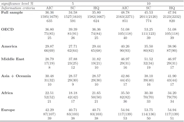
Table 5 reports the rates of rejection of the unit-root hypothesis using the Zivot and Andrews test. The rejection rates are significantly higher than the level of the test. The unit root is therefore much more often rejected if we take into account a structural break and this feature cannot be explained by a type-I testing error. The higher rates of rejection are obtained for the OECD, Middle-East and Europe. We note that the inclusion of breaks in the analysis does not modify the rank of each group with respect to the rejection rates.

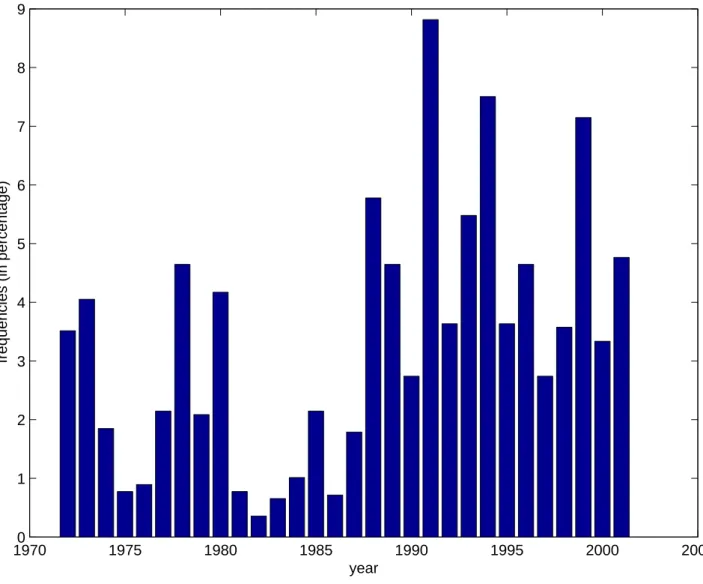
Each time the unit-root hypothesis is rejected, we apply the SupF and the ExpF tests of one structural change in order to ascertain this break. On the whole, these tests confirm the structural break. However, the hypothesis of an insignificant trend in the second part of the sample, that is to say after the break, is accepted only in a few cases, for instance for 38 differentials in Europe with a size of 5% for the unit-root test, which means that the cotrending condition is barely satisfied. To conclude, the Zivot and Andrews unit-root test with a structural break show that there are significantly fewer less unit-roots that previously estimated by simple ADF unit-root test. However, these results do not mean that we accept convergence for the different samples. As a matter of fact, the deterministic trend appears to be significant in many cases even after the break. Figure 2 displays the distribution of the date of these confirmed structural breaks. One can see that the bulk of the breaks appear after 1989, so in the second part of the sample. The highest number of breaks is observed in 1991. This feature could be linked to the acceleration of growth observed in the 1990’s in advanced as well as

(17)

emerging economies.

The non-rejection rates of the null hypothesis of stationarity with a level shift are reported in table 6. These rates are higher than the level of the test whatever the lag truncation parameter or the size of the test. They confirm that introducing a structural break significantly reduces the chance of accepting a unit-root in energy intensity differentials. When the stationarity hypothesis cannot be rejected, we apply the Supf and the Expf test for one structural break. In most of these cases, these tests confirm the hypothesis of one structural break. In those cases, we check if the constant become insignificant after the structural break and find that this hypothesis is most often rejected. To conclude, the results from the stationarity test with a break give more evidence of convergence than the previous results. However, the percentages of stationary differentials fluctuate between 51.22% (Middle east) and 19.05% (OCDE) which show that convergence cannot be considered as global for each of the samples we consider. Among each of these samples, there are some selected countries whose energy intensities are driven by the same trend but they do not share that trend with all other countries.

6 Conclusion

In this paper we used a pairwise test to assess convergence of energy intensities for a sample of 97 countries. Our method was to test if each energy intensities differential did not contain a stochastic or a deterministic trend or both. As we consider all energy intensities differentials, our results do not depend on the choice of a benchmark. Furthermore, we are able to detect if the acceptation of convergence in some cases can be attributed to an underlying process of convergence or merely arises from the error inherent in a statistical test. The use of unit-root as well as stationarity tests should give some robustness to our results. Empirical evidence concludes in favor of a non convergence hypothesis in the full sample but patterns of convergence appear in some sub-samples: Middle Eastern and, to a lesser extent, OECD countries. When allowing for a structural break in the data, convergence hypothesis is less strongly rejected.

These results have direct policy implications, namely that convergence cannot be taken for granted. In the pursuit of international environmental targets, this indicates that national energy and energy productivity policies should be regulated to reach a fairer allocation of resources.

As possible extensions to the present work it would be interesting to extend the analysis at the sectoral level, as in Miketa and Mulder (2005) and Mulder and De Groot (2007). Such an analysis might shed more light on the weak evidence of convergence depicted in the present study. Another possibility would be to introduce a methodological improvement, namely a more robust test of the trend (and thereby cotrending) hypothesis, as recently developed in Harvey et al. (2007).

(18)

Appendix: Sample and composition of country groups

• Group 1 : full sample of 97 countries

• Group 2 (OECD, 22 countries): Australia, Austria, Belgium, Canada, Denmark, Finland, France, Germany, Greece, Island, Ireland, Italy, Japan, Netherland, New Zealand, Norway, Portugal, Spain, Sweden, Switzerland, United Kingdom, USA.

• Group 3 (America, 22 countries): Argentina, Bolivia, Brazil, Canada, Chile, Colombia, Costa Rica, Dominican Republic, Ecuador, El Salvador, Guatemala, Honduras, Jamaica, Mexico, Nicaragua, Panama, Paraguay, Peru, Trinidad et Tobago, USA, Uruguay, Venezuela.

• Group 4 (Middle East, 12 countries): Bahrain, Brunei, Iran, Iraq, Israel, Jordan, Oman, Qatar, Saudi Arabia, Syria, Turkey, United Arab Emirates.

• Group 5 (Asia + Oceania, 15 countries): Australia, China, Hong Kong, India, Indonesia, South Korea, Japan, Malaysia, Nepal, New Zealand, Pakistan, Philippines, Singapore, Sri Lanka, Thai-land.

• Group 6 (Africa, 22 countries): Algeria, Benin, Cameroon, Democratic Republic of Congo, Re-public of congo, Cote d‘Ivoire, Egypt, Ethiopia, Gabon, Ghana, Kenya, Morocco, Mozambique, Nigeria, Senegal, South Africa, Sudan, Tanzania, Togo, Tunisia, Zambia, Zimbabwe.

• Group 7 (Europe, 23 countries): Belgium, Cyprus, Denmark, Finland, France, Germany, Greece, Hungary, Iceland, Ireland, Italy, Luxembourg, Malta, Netherlands, Norway, Poland, Portugal, Romania, Spain, Sweden, Switzerland, Turkey, United Kingdom.

(19)

1970 1975 1980 1985 1990 1995 2000 2005 −5 −4 −3 −2 −1 0 1 2

Figure 1: Cross-sectional representation of energy intensities (log of energy intensity relative to their cross sectional mean) for the 97 countries full sample

(20)

19700 1975 1980 1985 1990 1995 2000 2005 1 2 3 4 5 6 7 8 9 year

frequencies (in percentage)

Figure 2: Histogram of the dates of the confirmed structural breaks for the 97 countries sample from Zivot and Andrews (1992) unit-root test.

(21)

Table 1: Proportions of energy intensity differentials for which the unit-root hypothesis is rejected with ADF unit-root test.

significance level % 5 10

Information criteria AIC SC HQ AIC SC HQ

Full sample 9.68 9.45 10.00 15.76 14.56 15.63 110(451) 129(440) 122(466) 174(734) 189(678) 188(728) OECD 13.85 12.98 15.15 21.21 22.94 22.51 1(32) 1(30) 1(37) 3(49) 6(53) 4(52) America 6.92 5.62 6.49 13.42 9.95 11.68 2(16) 2(13) 2(15) 5(31) 3(23) 5(27) Middle East 12.12 15.15 12.12 25.76 24.24 24.24 2(8) 4(10) 3(8) 4(17) 6(16) 5(16) Asia + Oceania 4.76 5.71 5.71 12.38 13.33 13.33 0(5) 0(6) 0(6) 3(13) 3(14) 3(14) Africa 3.89 1.73 3.46 9.95 6.92 9.09 2(9) 0(4) 1(8) 6(23) 5(16) 7(21) Europe 15.81 14.23 15.41 28.46 25.29 27.66 7(40) 7(36) 4(39) 14(72) 12(64) 11(70)

Note a: The number on the first line is the rejection rate of the null hypothesis of a root. The

unit-root tests are based on an augmented Dickey-Fuller regression with an intercept and a linear trend, and are carried out at the 5% and 10% significance levels. Critical values are given by McKinnon (1996). The number of lagged differenced variables is chosen according to information criterion.

Note b: The numbers in brackets on the second line are the total number of country pairs for which

the unit-root hypothesis is rejected at the specified significance levels.

Note c : The numbers not in brackets on the second line are the number of country pairs for which

the hypothesis of a non significant trend is not rejected. Student tests of the significance of the linear trend are conducted at the 5% significance level.

(22)

Table 2: Proportions of energy intensity differentials for which the unit-root hypothesis is rejected with ADF-GLS (Eliot et al.)(1996) unit-root test.

Note a : The number on the first line is the rejection rate of the null hypothesis of a unit-root.

The unit-root tests are based on an augmented Dickey-Fuller regression with an intercept and a linear trend, and are carried out at the 5% and 10% significance levels. Critical values are given by McKinnon (1996). The number of lagged differenced variables is chosen according to information criterion.

Note b : The numbers in brackets on the second line are the total number of country pairs for which

(23)

Table 3: Proportions of energy intensity differentials for which the unit-root hypothesis is rejected with ADF-WS (Park and Fuller, 1995) unit-root test.

Note a : The unit-root tests are based on an augmented Dickey-Fuller regression with an intercept

and a linear trend, and are carried out at the 5% and 10% significance levels. Critical values are given by McKinnon (1996). The number of lagged differenced variables is chosen according to information criterion.

Note b : The numbers in brackets on the second line are the total number of country pairs for which

Table 4: Proportions of energy intensity differentials for which the stationarity hypothesis is not rejected using KPSS (1992) stationarity test with a constant

significance level 5 % 10 % l = 1 l = 2 l = 1 l = 2 Full sample 14.67 20.88 9.17 14.65 OECD 12.56 18.19 7.79 12.12 America 16.02 21.65 6.93 16.45 Middle East 28.79 34.85 24.24 27.27 Asia + Oceania 19.05 25.72 7.62 18.10 Africa 19.05 28.14 12.56 19.48 Europe 15.02 19.77 9.88 15.02

Note : The KPSS test statistics are applied to deviations of energy efficiencies differentials from a

constant mean. The critical values for the 5% and 10% significance levels are respectively equal to and are taken from Sephton (1995). The lag-window is equal to 1 and 2.

(24)

Table 5: Proportions of energy intensity differentials for which the Zivot and Andrews (1992) unit-root hypothesis with a break is rejected information criterion based selected lags

Full sample 36.36 34.58 35.80 48.78 45.53 47.94 1595(1679) 1527(1610) 1582(1667) 2163(2271) 2011(2120) 2123(2232) 635 591 624 851 774 820 OECD 36.80 39.39 36.36 51.08 53.25 51.08 75(85) 81(91) 74(84) 105(118) 111(123) 105(118) 25 26 25 40 39 39 America 29.87 27.71 29.44 40.26 35.50 38.96 66(69) 62(64) 65(68) 90(93) 80(82) 87(90) Middle East 28.79 37.88 31.82 46.97 51.52 46.97 17(19) 23(25) 19(21) 29(31) 32(34) 29(31) 8 12 10 16 19 17 Asia + Oceania 30.48 28.57 28.57 42.86 38.10 41.90 31(32) 29(30) 29(30) 44(45) 39(40) 43(44) 10 9 10 17 16 17 Africa 22.51 18.18 21.65 35.50 30.30 34.20 52(52) 42(42) 50(50) 82(82) 70(70) 79(79) 21 17 21 36 33 34 Europe 42.29 40.71 40.71 54.94 53.75 54.94 87(107) 83(103) 83(103) 117(139) 114(136) 117(139) 39 38 38 53 50 51

Notes a: The Zivot and Andrews (1992) unit-root tests with a structural break are based on the

changing growth model and are carried out at the 5% and 10% significance levels. The critical values are taken from Andrews(1996) and Bai and Perron (1998). The number of lagged differenced variables is chosen according to information criterion.

Note b: The numbers in brackets are the total number of country pairs for which the unit-root

hypothesis is rejected at the specified significance levels.

Note c : The numbers not in brackets are the number of country pairs for which the hypothesis of a

non significant trend is not rejected. Student tests of the significance of the linear trend are conducted at the 5% significance level.

(25)

Table 6: Proportions of energy intensity differentials for which the stationarity hypothesis is not rejected using Kurozumi (2002) stationarity test with a level shift

significance level 5 % 10 % l = 1 l = 2 l = 1 l = 2 Full sample 32.94 43.10 24.66 30.71 1464(1534) 1932(2007) 1080(1148) 1361(1430) 93 127 65 83 OECD 25.54 35.06 19.05 24.24 59(59) 80(81) 44(44) 56(56) 1 2 1 2 America 39.83 51.08 28.14 37.23 92(92) 118(118) 65(65) 86(86) 12 15 9 12 Middle East 43.94 51.52 27.27 37.88 29(29) 34(34) 18(18) 25(25) 4 4 4 4 Asia + Oceania 31.43 43.81 23.81 33.33 33(33) 46(46) 25(25) 35(35) 4 6 3 4 Africa 33.77 45.89 24.68 32.47 76(78) 103(106) 55(57) 73(75) 3 4 2 2 Europe 28.06 37.94 21.34 26.48 70(71) 94(96) 53(54) 66(66) 3 6 2 3

Note a : The Kurozumi (2002) stationarity test with a change in the intercept is applied to each

energy intensity differential. The critical values for the 5% and 10% significance levels are taken from Kurozumi (2002). The lag-windows are equal to 1 and 2.

Note b : The number on the first line is the percentage of non-rejection of the null stationarity with

a break in constant hypothesis.

Note c : The first number on the second line is the number of pairs for which the hypothesis of a break

in the constant is accepted by the Supf test of Andrews (1993) and Bai and Perron (1998, 2003). The number in brackets represents the number of pairs for which the stationarity with a break cannot be rejected.

Note d : The number on each third line is the number of stationary pairs for which the constant in