Score Bounded Monte-Carlo Tree Search
Tristan Cazenave and Abdallah SaffidineLAMSADE Université Paris-Dauphine
Paris, France
[email protected] [email protected]
Abstract. Monte-Carlo Tree Search (MCTS) is a successful algorithm used in
many state of the art game engines. We propose to improve a MCTS solver when a game has more than two outcomes. It is for example the case in games that can end in draw positions. In this case it improves significantly a MCTS solver to take into account bounds on the possible scores of a node in order to select the nodes to explore. We apply our algorithm to solving Seki in the game of Go and to Connect Four.
1
Introduction
Monte-Carlo Tree Search algorithms have been very successfully applied to the game of Go [7, 11]. They have also been used in state of the art programs for General Game Playing [9], for games with incomplete information such as Phantom Go [3], or for puzzles [4, 17, 5].
MCTS has also been used with an evaluation function instead of random playouts, in games such as Amazons [15] and Lines of Action [18].
In Lines of Action, MCTS has been successfully combined with exact results in a MCTS solver [19]. We propose to further extend this combination to games that have more than two outcomes. Example of such a game is playing a Seki in the game of Go: the game can be either lost, won or draw (i.e. Seki). Improving MCTS for Seki and Semeai is important for Monte-Carlo Go since this is one of the main weaknesses of current Monte-Carlo Go programs. We also address the application of our algorithm to Connect Four that can also end in a draw.
The second section deals with the state of the art in MCTS solver, the third section details our algorithm that takes bounds into account in a MCTS solver, the fourth section explains why Seki and Semeai are difficult for Monte-Carlo Go programs, the fifth section gives experimental results.
2
Monte-Carlo tree search solver
As the name suggests, MCTS builds a game tree in which each node is associated to a player, either Max or Min, and accordingly to values Qmaxand Qmin. As the tree
function is usually based on a combination of the mean of Monte Carlo playouts that went through the node [7, 13], and various heuristics such as All moves as first [10], or move urgencies [8, 6]. It can also involve an evaluation function as in [15, 18].
Monte-Carlo Tree Search is composed of four steps. First it descends a tree choos-ing at each node n the child of n maximizchoos-ing the value for the player in n. When it reaches a nodes with that has unexplored children, it adds a new leaf to the tree. Then the corresponding position is scored through the result of an evaluation function or a random playout. The score is backpropagated to the nodes that have been traversed during the descent of the tree.
MCTS is able to converge to the optimal play given infinite time, however it is not able to prove the value of a position if it is not associated to a solver. MCTS is not good at finding narrow lines of tactical play. The association to a solver enables MCTS to alleviate this weakness and to find some of them.
Combining exact values with MCTS has been addressed by Winands et al. in their MCTS solver [19]. Two special values can be assigned to nodes :+∞ and −∞. When a node is associated to a solved position (for example a terminal position) it is associated to+∞ for a won position and to −∞ for a lost position. When a max node has a won child, the node is solved and the node value is set to+∞. When a max node has all its children equal to −∞ it is lost and set to −∞. The descent of the tree is stopped as soon as a solved node is reached, in this case no simulation takes place and 1.0 is backpropagated for won positions, whereas -1.0 is backpropagated for lost ones.
Combining such a solver to MCTS improved a Lines Of Action (LOA) program, winning 65% of the time against the MCTS version without a solver. Winands et al. did not try to prove draws since draws are exceptional in LOA.
3
Integration of score bounds in MCTS
We assume the outcomes of the game belong to an interval[minscore, maxscore] of IR, the player Max is trying to maximize the outcome while the player Min is trying to minimize the outcome.
In the following we are supposing that the tree is a minimax tree. It can be a partial tree of a sequential perfect information deterministic zero-sum game in which each node is either a max-node when the player Max is to play in the associated position or a min-node otherwise. Note that we do not require the child of a max-node to be a min-node, so a step-based approach to MCTS (for instance in Arimaa [14]) is possible. It can also be a partial tree of a perfect information deterministic one player puzzle. In this latter case, each node is a max-node and Max is the only player considered.
We assume that there are legal moves in a game position if and only if the game position is non terminal. Nodes corresponding to terminal game positions are called terminal nodes. Other nodes are called internal nodes.
Our algorithm adds score bounds to nodes in the MCTS tree. It needs slight modi-fications of the backpropagation and descent steps. We first define the bounds that we consider and express a few desired properties. Then we show how bounds can be ini-tially set and then incrementally adapted as the available information grows. We then
show how such knowledge can be used to safely prune nodes and subtrees and how the bounds can be used to heuristically bias the descent of the tree.
3.1 Pessimistic and optimistic bounds
For each node n, we attach a pessimistic (noted pess(n)) and an optimistic (noted opti(n)) bound to n. Note that optimistic and pessimistic bounds in the context of game tree search were first introduced by Hans Berliner in his B* algorithm [2]. The names of the bounds are defined after Max’s point of view, for instance in both max-and min-nodes, the pessimistic bound is a lower bound of the best achievable outcome for Max (assuming rational play from Min). For a fixed node n, the boundpess(n) is increasing (resp.opti(n) is decreasing) as more and more information is available. This evolution is such that no false assumption is made on the expectation of n : the outcome of optimal play from node n on, notedreal(n), is always between pess(n) and opti(n). That is pess(n) ≤ real(n) ≤ opti(n). If there is enough time allocated to informa-tion discovering in n,pess(n) and opti(n) will converge towards real(n). A position corresponding to a node n is solved if and only ifpess(n) = real(n) = opti(n).
If the node n is terminal then the pessimistic and the optimistic values correspond to the score of the terminal positionpess(n) = opti(n) = score(n). Initial bounds for in-ternal nodes can either be set to the lowest and highest scorespess(n) = minscore and opti(n) = maxscore, or to some values given by an appropriate admissible heuristic [12]. At a given time, the optimistic value of an internal node is the best possible out-come that Max can hope for, taking into account the information present in the tree and assuming rational play for both player. Conversely the pessimistic value of an internal node is the worst possible outcome that Max can fear, with the same hypothesis. There-fore it is sensible to update bounds of internal nodes in the following way.
If n is an internal max-node then pess(n) := maxs∈children(n)pess(s)
opti(n) := maxs∈children(n)opti(s)
If n is an internal min-node then pess(n) := mins∈children(n)pess(s)
opti(n) := mins∈children(n)opti(s)
3.2 Updating the tree
Knowledge about bounds appears at terminal nodes, for the pessimistic and optimistic values of a terminal node match its real value. This knowledge is then recursively up-wards propagated as long as it adds information to some node. Using a fast incremental algorithm enables not to slow down the MCTS procedure.
Let s be a recently updated node whose parent is a max-node n. Ifpess(s) has just been increased, then we might want to increasepess(n) as well. It happens when the new pessimistic bound for s is greater than the pessimistic bound for n :pess(n) := max(pess(n), pess(s)). If opti(s) has just been decreased, then we might want to de-creaseopti(n) as well. It happens when the old optimistic bound for s was the greatest among the optimistic bounds of all children of n.opti(n) := maxs∈children(n)opti(s).
The converse update process takes place when s is the child of a min-node.
When n is not fully expanded, that is when some children of n have not been created yet, a dummy child d such thatpess(d) = minscore and opti(d) = maxscore can be added to n to be able to compute conservative bounds for n despite bounds for some children being unavailable.
Algorithm 1 Pseudo-code for propagating pessimistic bounds
procedure prop-pess arguments node s
if s is not the root node then
Let n be the parent of s Let old_pess:= pess(n)
if old_pess <pess(s) then
if n is a Max node then
pess(n) := pess(s) prop-pess(n)
else
pess(n) := mins′∈children(n)pess(s′) if old_pess >pess(n) then
prop-pess(n)
end if end if end if end if
Algorithm 2 Pseudo-code for propagating optimistic bounds
procedure prop-opti arguments node s
if s is not the root node then
Let n be the parent of s Let old_opti:= opti(n)
if old_opti >opti(s) then
if n is a Max node then
opti(n) := maxs′∈children(n)opti(s ′
)
if old_opti >opti(n) then prop-opti(n) end if else opti(n) := opti(s) prop-opti(n) end if end if end if
3.3 Pruning nodes with alpha-beta style cuts
Once pessimistic and optimistic bounds are available, it is possible to prune subtrees using simple rules. Given a max-node (resp. min-node) n and a child s of n, the subtree starting at s can safely be pruned ifopti(s) ≤ pess(n) (resp. pess(s) ≥ opti(n)).
To prove that the rules are safe, let’s suppose n is an unsolved max-node and s is a child of n such thatopti(s) ≤ pess(n). We want to prove it is not useful to explore the child s. On the one hand, n has at least one child left unpruned. That is, there is at least a child of n, s+, such thatopti(s′) > pess(n). This comes directly from the fact that
as n is unsolved,opti(n) > pess(n), or equivalently maxs+∈children(n)opti(s+) >
pess(n). s+is not solved. On the other hand, let us show that there exists at least one
other child of n better worth choosing than s. By definition of the pessimistic bound of n, there is at least a child of n, s′, such thatpess(s′) = pess(n). The optimistic
outcome in s is smaller than the pessimistic outcome in s′ : real(s) ≤ opti(s) ≤
pess(s′) ≤ real(s′). Now either s 6= s′and s′can be explored instead of s with no loss,
or s= s′and s is solved and does not need to be explored any further, in the latter case
s+could be explored instead of s.
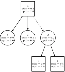
An example of a cut node is given in Figure 1. In this figure, the min-node d has a solved child (f ) with a 0.5 score, therefore the best Max can hope for this node is 0.5. Node a has also a solved child (c) that scores 0.5. This makes node d useless to explore since it cannot improve upon c.
a pess = 0.5 opti = 1.0 c pess = 0.5 opti = 0.5 b pess = 0.0 opti = 1.0 e pess = 0.0 opti = 1.0 d pess = 0.0 opti = 0.5 f pess = 0.5 opti = 0.5
Fig. 1. Example of a cut. The d node is cut because its optimistic value is smaller or equal to the
3.4 Bounds based node value bias
The pessimistic and optimistic bounds of nodes can also be used to influence the choice among uncut children in a complementary heuristic manner. In a max-node n, the cho-sen node is the one maximizing a value function Qmax.
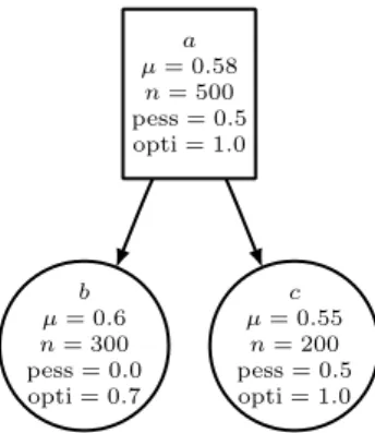
In the following example, we assume the outcomes to be reals from[0, 1] and for sake of simplicity the Q function is assumed to be the mean of random playouts. Figure 2 shows an artificial tree with given bounds and given results of Monte-Carlo evalua-tions. The node a has two children b and c. Random simulations seem to indicate that the position corresponding to node c is less favorable to Max than the position corre-sponding to b. However the lower and upper bounds of the outcome in c and b seem to mitigate this estimation.
a µ= 0.58 n= 500 pess = 0.5 opti = 1.0 c µ= 0.55 n= 200 pess = 0.5 opti = 1.0 b µ= 0.6 n= 300 pess = 0.0 opti = 0.7
Fig. 2. Artificial tree in which the bounds could be useful to guide the selection.
This example intuitively shows that taking bounds into account could improve the node selection process. It is possible to add bound induced bias to the node values of a son s of n by setting two bias terms γ and δ, and rather using adapted Q′ node values
defined as Q′
max(s) = Qmax(s) + γ pess(s) + δ opti(s) and Q′min(s) = Qmin(s) −
γopti(s) − δ pess(s).
4
Why Seki and Semeai are hard for MCTS
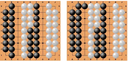
The figure 3 shows two Semeai. The first one is unsettled, the first player wins. In this position, random playouts give a probability of 0.5 for Black to win the Semeai if he plays the first move of the playout. However if Black plays perfectly he always wins the Semeai.
The second Semeai of figure 3 is won for Black even if White plays first. The prob-ability for White to win the Semeai in a random game starting with a White move is 0.45. The true value with perfect play should be 0.0.
We have written a dynamic programming program to compute the exact probabili-ties of winning the Semeai for Black if he plays first. A probability p of playing in the
Fig. 3. An unsettled Semeai and Semeai lost for White.
Semeai is used to model what would happen on a 19x19 board where the Semeai is only a part of the board. In this case playing moves outside of the Semeai during the playout has to be modeled.
The table 1 gives the probabilities of winning the Semeai for Black if he plays first according to the number of liberties of Black (the rows) and the number of liberties of White (the column). The table was computed with the dynamic programming algorithm and with a probability p = 0.0 of playing outside the Semeai. We can now confirm, looking at row 9, column 9 that the probability for Black to win the first Semeai of figure 3 is 0.50.
Own liberties Opponent liberties
1 2 3 4 5 6 7 8 9 1 1.00 0.00 0.00 0.00 0.00 0.00 0.00 0.00 0.00 2 1.00 0.50 0.30 0.20 0.14 0.11 0.08 0.07 0.05 3 1.00 0.70 0.50 0.37 0.29 0.23 0.18 0.15 0.13 4 1.00 0.80 0.63 0.50 0.40 0.33 0.28 0.24 0.20 5 1.00 0.86 0.71 0.60 0.50 0.42 0.36 0.31 0.27 6 1.00 0.89 0.77 0.67 0.58 0.50 0.44 0.38 0.34 7 1.00 0.92 0.82 0.72 0.64 0.56 0.50 0.45 0.40 8 1.00 0.93 0.85 0.76 0.69 0.62 0.55 0.50 0.45 9 1.00 0.95 0.87 0.80 0.73 0.66 0.60 0.55 0.50
In this table, when the strings have six liberties or more, the values for lost positions are close to the values for won positions, so MCTS is not well guided by the mean of the playouts.
5
Experimental Results
In order to apply the score bounded MCTS algorithm, we have chosen games that can often finish as draws. Such two games are playing a Seki in the game of Go and Connect Four. The first subsection details the application to Seki, the second subsection is about Connect Four.
5.1 Seki problems
We have tested Monte-Carlo with bounds on Seki problems since there are three possi-ble exact values for a Seki: Won, Lost or Draw. Monte-Carlo with bounds can only cut nodes when there are exact values, and if the values are only Won and Lost the nodes are directly cut without any need for bounds.
Solving Seki problems has been addressed in [16]. We use more simple and easy to define problems than in [16]. Our aim is to show that Monte-Carlo with bounds can improve on Monte-Carlo without bounds as used in [19].
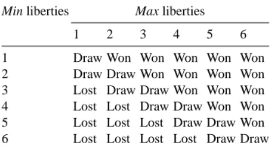
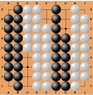
We used Seki problems with liberties for the players ranging from one to six lib-erties. The number of shared liberties is always two. The Max player (usually Black) plays first. The figure 4 shows the problem that has three liberties for Max (Black), four liberties for Min (White) and two shared liberties. The other problems of the test suite are very similar except for the number of liberties of Black and White. The results of these Seki problems are given in table 2. We can see that when Max has the same number of liberties than Min or one liberty less, the result is Draw.
Min liberties Max liberties
1 2 3 4 5 6
1 Draw Won Won Won Won Won
2 Draw Draw Won Won Won Won 3 Lost Draw Draw Won Won Won 4 Lost Lost Draw Draw Won Won 5 Lost Lost Lost Draw Draw Won 6 Lost Lost Lost Lost Draw Draw
Table 2. Results for Sekis with two shared liberties
The first algorithm we have tested is simply to use a solver that cuts nodes when a child is won for the color to play as in [19]. The search was limited to 1 000 000 playouts. Each problem is solved thirty times and the results in the tables are the average
Fig. 4. A test seki with two shared liberties, three liberties for the Max player (Black) and four
liberties for the Min player (White).
number of playouts required to solve a problem. An optimized Monte-Carlo tree search algorithm using the Rave heuristic is used. The results are given in table 3. The result corresponding to the problem of figure 4 is at row labeled 4 min lib and at column labeled 3 max lib, it is not solved in 1 000 000 playouts.
Min liberties Max liberties
1 2 3 4 5 6 1 359 479 1535 2059 10 566 25 670 2 1389 11 047 12 627 68 718 98 155 28 9324 3 7219 60 755 541 065 283 782 516 514 79 1945 4 41 385 422 975 >1 000 000 >1 000 000 >989 407 >999 395 5 275 670 >1 000 000 >1 000 000 >1 000 000 >1 000 000 >1 000 000 6 >1 000 000 >1 000 000 >1 000 000 >1 000 000 >1 000 000 >1 000 000
Table 3. Number of playouts for solving Sekis with two shared liberties
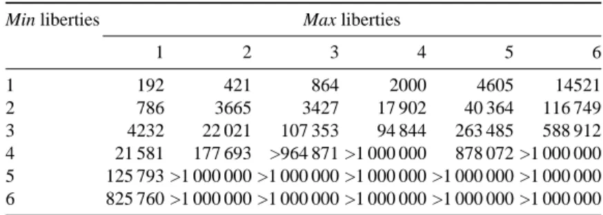
The next algorithm uses bounds on score, node pruning and no bias on move se-lection (i.e. γ = 0 and δ = 0). Its results are given in table 4. Table 4 shows that Monte-Carlo with bounds and node pruning works better than a Monte-Carlo solver without bounds.
Comparing table 4 to table 3 we can also observe that Monte-Carlo with bounds and node pruning is up to five time faster than a simple Monte-Carlo solver. The problem with three Min liberties and three Max liberties is solved in 107 353 playouts when it is solved in 541 065 playouts by a plain Monte-Carlo solver.
Min liberties Max liberties
1 2 3 4 5 6 1 192 421 864 2000 4605 14521 2 786 3665 3427 17 902 40 364 116 749 3 4232 22 021 107 353 94 844 263 485 588 912 4 21 581 177 693 >964 871 >1 000 000 878 072 >1 000 000 5 125 793 >1 000 000 >1 000 000 >1 000 000 >1 000 000 >1 000 000 6 825 760 >1 000 000 >1 000 000 >1 000 000 >1 000 000 >1 000 000
Table 4. Number of playouts for solving Sekis with two shared liberties, bounds on score, node
pruning, no bias
The third algorithm uses bounds on score, node pruning and biases move selection with δ = 10000. The results are given in table 5. We can see in this table that the number of playouts is divided by up to ten. For example the problem with three Max lib and three Min lib is now solved in 9208 playouts (it was 107 353 playouts without biasing move selection and 541 065 playouts without bounds). We can see that eight more problems can be solved within the 1 000 000 playouts limit.
Min liberties Max liberties
1 2 3 4 5 6 1 137 259 391 1135 2808 7164 2 501 1098 1525 3284 13 034 29 182 3 1026 5118 9208 19 523 31 584 141 440 4 2269 10 094 58 397 102 314 224 109 412 043 5 6907 27 947 127 588 737 774 >999 587 >1 000 000 6 16 461 85 542 372 366 >1 000 000 >1 000 000 >1 000 000
Table 5. Number of playouts for solving Sekis with two shared liberties, bounds on score, node
pruning, biasing with γ= 0 and δ = 10000
5.2 Connect Four
Connect Four was solved for the standard size 7x6 by L. V. Allis in 1988 [1]. We tested a plain MCTS Solver as described in [19] (plain), a score bounded MCTS with
alpha-beta style cuts but no selection guidance that is with γ= 0 and δ = 0 (cuts) and a score bounded MCTS with cuts and selection guidance with γ = 0 and δ = −0.1 (guided cuts). We tried multiple values for γ and δ and we observed that the value of γ does not matter much and that the best value for δ was consistently δ= −0.1. We solved various small sizes of Connect Four. We recorded the average over thirty runs of the number of playouts needed to solve each size. The results are given in table 6.
Size
3 × 3 3 × 4 4 × 3 4 × 4 plain MCTS Solver 2700.9 26 042.7 227 617.6 >5 000 000 MCTS Solver with cuts 2529.2 12 496.7 31 772.9 386 324.3 MCTS Solver with guided cuts 1607.1 9792.7 24 340.2 351 320.3
Table 6. Comparison of solvers for various sizes of Connect Four
Concerning 7x6 Connect Four we did a 200 games match between a Monte-Carlo with alpha-beta style cuts on bounds and a Monte-Carlo without it. Each program played 10 000 playouts before choosing each move. The result was that the program with cuts scored 114.5 out of 200 against the program without cuts (a win scores 1, a draw scores 0.5 and a loss scores 0).
6
Conclusion and Future Works
We have presented an algorithm that takes into account bounds on the possible values of a node to select nodes to explore in a MCTS solver. For games that have more than two outcomes, the algorithm improves significantly on a MCTS solver that does not use bounds.
In our solver we avoided solved nodes during the descent of the MCTS tree. As [19] points out, it may be problematic for a heuristic program to avoid solved nodes as it can lead MCTS to overestimate a node.
It could be interesting to make γ and δ vary with the number of playout of a node as in RAVE. We may also investigate alternative ways to let score bounds influence the child selection process, possibly taking into account the bounds of the father.
We currently backpropagate the real score of a playout, it could be interesting to adjust the propagated score to keep it consistent with the bounds of each node during the backpropagation.
Acknowledgments
This work has been supported by French National Research Agency (ANR) through COSINUS program (project EXPLO-RA ANR-08-COSI-004)
References
1. L. Victor Allis. A knowledge-based approach of connect-four the game is solved: White wins. Masters thesis, Vrije Universitat Amsterdam, Amsterdam, The Netherlands, October 1988.
2. Hans J. Berliner. The B* tree search algorithm: A best-first proof procedure. Artif. Intell., 12(1):23–40, 1979.
3. Tristan Cazenave. A Phantom-Go program. In Advances in Computer Games 2005, volume 4250 of Lecture Notes in Computer Science, pages 120–125. Springer, 2006.
4. Tristan Cazenave. Reflexive monte-carlo search. In Computer Games Workshop, pages 165– 173, Amsterdam, The Netherlands, 2007.
5. Tristan Cazenave. Nested monte-carlo search. In IJCAI, pages 456–461, 2009.
6. Guillaume Chaslot, L. Chatriot, C. Fiter, Sylvain Gelly, Jean-Baptiste Hoock, J. Perez, Arpad Rimmel, and Olivier Teytaud. Combiner connaissances expertes, hors-ligne, transientes et en ligne pour l’exploration Monte-Carlo. Apprentissage et MC. Revue d’Intelligence
Artifi-cielle, 23(2-3):203–220, 2009.
7. Rémi Coulom. Efficient selectivity and back-up operators in monte-carlo tree search. In
Computers and Games 2006, Volume 4630 of LNCS, pages 72–83, Torino, Italy, 2006.
Springer.
8. Rémi Coulom. Computing Elo ratings of move patterns in the game of Go. ICGA Journal, 30(4):198–208, December 2007.
9. Hilmar Finnsson and Yngvi Björnsson. Simulation-based approach to general game playing. In AAAI, pages 259–264, 2008.
10. Sylvain Gelly and David Silver. Combining online and offline knowledge in UCT. In ICML, pages 273–280, 2007.
11. Sylvain Gelly and David Silver. Achieving master level play in 9 x 9 computer go. In AAAI, pages 1537–1540, 2008.
12. P. Hart, N. Nilsson, and B. Raphael. A formal basis for the heuristic determination of mini-mum cost paths. IEEE Trans. Syst. Sci. Cybernet., 4(2):100–107, 1968.
13. L. Kocsis and C. Szepesvàri. Bandit based monte-carlo planning. In ECML, volume 4212 of
Lecture Notes in Computer Science, pages 282–293. Springer, 2006.
14. Tomáš Kozelek. Methods of MCTS and the game Arimaa. Master’s thesis, Charles Univer-sity in Prague, 2009.
15. Richard J. Lorentz. Amazons discover monte-carlo. In Computers and Games, pages 13–24, 2008.
16. Xiaozhen Niu, Akihiro Kishimoto, and Martin Müller. Recognizing seki in computer go. In
ACG, pages 88–103, 2006.
17. Maarten P. D. Schadd, Mark H. M. Winands, H. Jaap van den Herik, Guillaume Chaslot, and Jos W. H. M. Uiterwijk. Single-player monte-carlo tree search. In Computers and Games, pages 1–12, 2008.
18. Mark H. M. Winands and Yngvi Björnsson. Evaluation function based Monte-Carlo LOA. In Advances in Computer Games, 2009.
19. Mark H. M. Winands, Yngvi Björnsson, and Jahn-Takeshi Saito. Monte-carlo tree search solver. In Computers and Games, pages 25–36, 2008.