tree-based ensemble methods
Francis Maes, Pierre Geurts, and Louis Wehenkel
University of Li`ege
Dept. of Electrical Engineering and Computer Science Institut Montefiore, B28, B-4000, Li`ege - Belgium
Abstract. Feature generation is the problem of automatically construct-ing good features for a given target learnconstruct-ing problem. While most feature generation algorithms belong either to the filter or to the wrapper ap-proach, this paper focuses on embedded feature generation. We propose a general scheme to embed feature generation in a wide range of tree-based learning algorithms, including single decision trees, random forests and tree boosting. It is based on the formalization of feature construction as a sequential decision making problem addressed by a tractable Monte Carlo search algorithm coupled with node splitting. This leads to fast algorithms that are applicable to large-scale problems. We empirically analyze the performances of these tree-based learners combined or not with the feature generation capability on several standard datasets. Keywords: Embedded Feature Generation, Monte Carlo Search, Deci-sion Trees, Random Forests, Tree Boosting
1
Introduction
It is often admitted that the successful application of supervised learning depends at least as much on the features chosen to describe the inputs of objects than on the adopted learning algorithm. In addition to improving the accuracy of the resulting models, a proper choice of features can also lead to more compact models which often gain in interpretability. In practice, feature engineering - the process of identifying a good set of features for a given learning task - is usually performed manually based on problem expertise, which makes it more an art than a science. In order to remedy this situation, a number of algorithms for automatic feature generation have been proposed since the nineties (see [15, 19] for examples of early work on this topic).
Most proposed approaches for automatic feature generation1take the form of a preprocessing: before doing actual learning, some kind of search is performed in a space of candidate features in order to construct a (typically small) set of features that are expected to help learning better models. Proposed approaches for this preprocessing can be classified in two categories: filters and wrappers
1
[6]. In the former case, the search for good features is performed on the basis of general statistics, logical or information content criteria (see [8] for example), while the latter case directly relies on the performance of the target learning algorithm to guide search through the feature space. Examples of wrappers in-clude the work of [16] based on wrapping the kNN learning algorithm or the work of [10] where the wrapped learning algorithm is a C4.5 decision tree. More recently the authors of [18] proposed an algorithm for joint feature construction and feature selection, wrapping either C4.5, kNN or a Bayesian classifier. Some form of genetic programming is used in most of these works, in which individuals are typically feature sets represented as a forest composed of n trees, each tree describing one particular feature.
Feature generation is closely related to feature selection and, while feature selection methods may also be classified as filters or wrappers, the last decade has seen an increasing interest for so-called embedded feature selection meth-ods. In these latter methods, the feature selection task is embedded within the learning algorithm formulation, for example through the use of a L1-norm based regularization term added to an average loss term to yield the learning objec-tive function [13]. Embedded methods may offer some advantages over filters and wrappers, including much better scaling properties and better theoretical under-standing. Surprisingly however, embedded methods have received little attention in the field of feature generation. To our best knowledge, the few embedded fea-ture generation methods proposed so far are built around single decision tree induction. As an example, it is proposed in [5] to invoke a genetic programming algorithm to find the best splitting feature at each node during decision tree in-duction. In this case, feature generation is not seen anymore as a preprocessing step, but is instead tightly integrated within the learning process.
In this paper, we propose a general scheme to embed in a flexible way feature generation in a wide range of tree-based supervised learning algorithms includ-ing sinclud-ingle decision trees, random forests and common forms of tree boostinclud-ing. We emphasize our analysis on the two latter types of algorithms, since numer-ous studies show that they clearly outperform single decision trees in terms of classification accuracy [2].
Both random forests and tree boosting rely on some form of vote over a set of predictors and they are often the most effective when the individual predic-tors are only of moderate quality: boosting is based on the combination of many weak classifiers and random forests rely on randomization to reduce the correla-tion of ensemble terms. As a consequence, it may be unnecessary and possibly counterproductive to invest a huge computational budget in the search over the feature space in the context of these methods. Therefore, instead of using compu-tationally complex genetic programming algorithms, we propose to use a Monte Carlo search algorithm which budget may be controlled so as to both weakly and efficiently explore the feature space at each tree-node when constructing model terms in random forests or in tree boosting. Our approach thus leads to a fast integrated learning and feature generation procedure that scales well to large scale problems and adapts well to the properties of tree-based ensemble
methods, while it works also with single trees. We show empirically that embed-ding this feature search into single trees, random forests and tree boosting yields significant improvements over these algorithms in their basic forms.
The rest of this paper is organized as follows. Section 2 introduces notations and formulates the learning problem we address. Section 3 motivates the main principles of our approach for embedded feature generation. Section 4 formalizes feature generation as a sequential decision making problem and describes Monte Carlo search algorithms to explore the feature space both efficiently and with controlled strength. Section 5 presents an empirical evaluation of our algorithms using several tree-based learning algorithms and Section 6 concludes.
2
Problem formulation
We consider supervised learning where, given a dataset S = {(x(i), y(i))} i∈[1,N ] of samples (x, y) ∈ X × Y i.i.d. from a distribution DX ,Y, the aim is to infer a classifier h ∈ H to minimize the expected risk: E(x,y)∼DX ,Y{∆(h(x), y)}.
Clas-sically in supervised learning, the input objects x are vectors of numerical or categorical features that can directly be exploited by the learning algorithm. This assumes that feature engineering has already been done when formulating the learning problem. In our context, the aim is to integrate feature generation within the learning process and we thus make no strong assumptions on the nature of X . An input object x ∈ X is an n-tuple of properties x = (x1, . . . , xn), where each xi belongs to the space Xi that can either be continuous, discrete or structured. Properties can for example be raw signals such as images or struc-tured data such as trees and graphs. Classical categorical or numerical data also naturally fit in this framework.
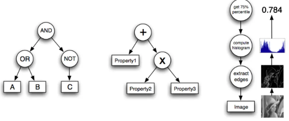
In order to bring the capacity of feature generation to the learning algorithm, we expect the user to provide a set of constructor functions, as proposed in [11]. These functions can be mathematical, logical and/or domain-specific and serve as the basis for feature generation. Formally, a constructor function of arity a is a triplet (I, O, F ) where I is the input domain (X1× · · · × Xk), O is the output domain and F is a function F : I → O. As an example, addition of two scalars has arity k = 2 and is defined as (I, O, F ) = (R×R, R, F (x, y) = x+y). Constructor functions can either be applied to the input properties xi or to the results of other constructor functions. This naturally leads to tree-structured features as illustrated by Figure 1. Note that this way of generating features is rather general and enables to encode complex processing pipelines [14].
3
A general scheme for embedding feature generation
Most previous automatic feature generation algorithms are preprocessings that aim at constructing a mapping φ : X → Z that extracts a set of relevant features adapted to the targeted learning algorithm (e.g. typically, we have Z ⊂ Rd). Learning is then performed on the basis of the modified data set {φ(x(i)), y(i)}
Fig. 1. Examples of constructed features for three different domains: booleans, real-valued attributes and images.
h(φ(x)) ∈ Y. This paper proposes a scheme to do both feature generation and learning in an integrated way, so as to solve the following problem: given the dataset whose inputs are general properties, and a set of constructor functions, infer a classifier h : X → Y to minimize the expected risk.
Random forests, boosted stumps and boosted decision trees are among the top-performing and most widely used supervised learning methods nowadays [2]. These algorithms all rely on decision trees, which involve splitting the dataset recursively by testing one variable at a time. At this level, instead of testing the raw input variables of the problem, our approach consists in splitting the local dataset on the basis of locally constructed features, along the ideas of [5].
Table 1 summarizes the characteristics of the splitting procedure of well-known tree-based supervised learning algorithms2. In single decision trees and random forests, splits are constructed by searching the threshold optimizing the information gain for each candidate variable and by selecting the variable with maximal information gain. Random forests [1] are forests constructed using bagging and random subspaces: when building a node, only a subset of the (non-constant) attributes are considered as candidates for making the split. In addition to random subspaces, extremely randomized trees [7] introduce randomization by selecting splitting thresholds randomly, which often leads to improved models. In the two boosting methods, the splitting criterion depends on both the selected samples D and on their current weight W [17].
Our approach which is detailed in Section 4 consists in testing a small and randomized part of the feature space to weakly optimize the split scores of Table 1, during each node creation. Note that, except single decision trees, all these learning algorithms are ensemble approaches that rely on some form of majority
2 Note that while we only consider numerical attributes for the sake of simplicity, the
Method Abbr. Split score Optimizer Single decision Tree ST maxt∈XiInf oGain(S, xi≤ t) Exhaustive
Random Forest RF maxt∈XiInf oGain(S, xi≤ t) Subset Extremely randomized Trees ET Inf oGain(S, xi≤ t) where t ∼ UXi Subset
Boosted Stumps BS maxt∈XiEdge(S, W, xi≤ t) Exhaustive Boosted decision Trees BT maxt∈XiEdge(S, W, xi≤ t) Exhaustive Table 1. Tree-based learning algorithms with associated splitting procedures.
vote to perform predictions. We believe that in this context, performing only a weak optimization over the feature space makes sense for various reasons:
– With all ensemble models, learning typically involves making several thou-sands of splits. So, even if only, say, 1% of a feature subspace is looked at each node, the whole subspace may still be visited multiple times during the entire learning procedure, and each of its elements may have multiple chances to be selected.
– Random forests and extremely randomized trees already rely on random subspaces to introduce randomization, which was shown to lead to improved generalization accuracy. Hence, exploring weakly the feature space is a nat-ural extension of these algorithms that should conserve their advantages. – With boosting, it is well known that the stronger the base learner is, the
higher the chances of overfitting are. When embedding automatic feature generation into boosting, this problem is particularly relevant since the fea-ture space may be highly expressive. Weak exploration of the feafea-ture space is a way to ensure that, even with very expressive candidate features, the base learner remains weak, hence reducing the risk of overfitting.
In the context of ensemble models, we therefore suggest that it may be unnec-essary or even counter-productive to use computationally intensive optimization algorithms (e.g. genetic programming, or sophisticated heuristic search) as tradi-tionally done in automatic feature generation. To explore this idea, the following section proposes fast randomized feature generation algorithms invoked locally during tree growing and in Section 5 we study them empirically.
4
Feature generation algorithms
We define first the feature grammar, then their generation as a sequential decision-making problem, and finally address this problem by Monte Carlo search.
4.1 Feature grammar using reverse polish notation
Reverse polish notation (RPN) is a representation of expressions wherein every operator follows all of its operands. For instance, the RPN representation of the feature c × (a + b), where a, b and c are input properties and + and × are constructor functions, is the sequence of symbols [c, a, b, +, ×]. This way of
Algorithm 1 RPN evaluation
Require: f ∈ AD: a feature of size D Require: x ∈ X : input properties
stack ← ∅
for d = 1 to D do
if αdis an input property then
Push the value of αd onto the stack
else
Let k be the arity of constructor αd
if |stack| < k then syntax error else
Pop the top k values from the stack,
apply αdto these operands and push the result onto the stack
end if end if end for if |stack| 6= 1 then syntax error else return top(stack) end if
representing expressions is also known as postfix notation and is parenthesis-free as long as operator arities are fixed, which makes it simpler to manipulate than its counterparts, prefix notation and infix notation.
Let A be the set of symbols composed of input properties and constructor functions. A feature f is a finite sequence of symbols of A: f = [α1, . . . , αD] ∈ A∗. The size of a feature f is its number D of symbols. The evaluation of an RPN sequence relies on a stack and is depicted in Algorithm 1. This evaluation fails either if the stack does not contain enough operands when a constructor function is used or if the stack contains more than one single element at the end of the process. Feature [a, ×] leads to the first kind of error: the function × of arity 2 is applied with a single operand. Feature [a, a, a] leads to the second kind of error: evaluation finishes with three different elements on the stack. Features avoiding both kinds of errors are syntactically correct and are denoted f ∈ F ⊂ A∗.
4.2 Feature generation as a sequential decision-making problem
We rely on RPN to formalize feature generation as a sequential decision-making problem. Thanks to this formalization, feature generation can be considered as a “one-player game” and solved using Monte Carlo search algorithms. In our approach, we expect the user to provide D, the maximal constructed feature size, i.e. the length of the longest features which will be considered as candidates. Given D, our sequential decision-making problem is defined as follows:
State Valid actions
|stack| = 0 I
|stack| = 1 & d 6= D − 1 I,U,⊥ |stack| = 1 & d = D − 1 U,⊥ |stack| ∈ [2, D − d[ I,U,B
|stack| = D − d U,B
|stack| = D − d + 1 B
Table 2. Set of valid actions depending on the current state. Symbols are classified into I nput properties, U nary function constructors and B inary function constructors. |stack| denotes the size of the current stack and d the length of the current RPN sequence. If the stack does not contain at least one element (resp. two elements), the unary functions (resp. binary functions) are excluded. When approaching the horizon D, input properties are excluded, or binary functions are forced to avoid finishing with too many elements on the stack.
– State space: a state s is an RPN subsequence: s = [α1, . . . , αd] ∈ A∗ with d ≤ D. The initial state is the empty sequence s0= ∅.
– Action space: the action space is A ∪ {⊥}, where ⊥ is a special symbol to denote the end of a sequence. Given state s, we only consider a subset AD
s ⊂ A of valid actions to avoid the two syntax errors described earlier and to respect the constructor function typing constraints. Table 4.2 illustrates the set of valid actions AD
s ⊂ A in a simple case containing only unary and binary constructor functions that all operate on the same domain (e.g. only functions operating on real numbers). The following pre-processing can be used to compute the sets As in the general case. First, generate a tree of all the possible states of the stack for depths d = 0, 1, . . . , D. The state of the stack is composed of a vector of variable domains; it does not depend on any particular input x ∈ X . Then, prune this tree by removing recursively all nodes leading to no valid RPN sequences. Given a particular state s, identify the corresponding state of the stack in this pruned tree and build As accordingly.
– Transition function: if the action ⊥ is selected, we enter a final state defining feature f = s. Otherwise, the selected symbol is appended to the current RPN subsequence s.
– Reward: it is obtained when entering a final state and corresponds to the score computed by the target learning algorithm (see Table 1).
4.3 Monte Carlo search for feature generation
Monte Carlo search algorithms for making optimal decisions are receiving an increasing interest in various fields of artificial intelligence [4], essentially due to their ability to combine the precision of tree search with the generality of random simulations. As a first step towards studying the application of these
Algorithm 2 Random, step and look-ahead feature generation algorithms
Require: budget K
Require: maximal feature size D function randomSimulation(state s)
while s is not a final state do a ∼ UAD
s . Sample valid action randomly
s ← s :: a . Append symbol to s end while return s end function function stepSimulation(state s) r∗← −∞; f∗← ∅; d ← 1
while s is not a final state do
f ← randomSimulation(s) . Fill with random simulation if score(f ) > r∗ then f∗← f ; r∗← score(f ) end if
s ← s :: f∗[d] . Append the d-th symbol of the best constructed feature d ← d + 1 end while return f∗ end function function lookAheadSimulation(state s) r∗← −∞; f∗← ∅; d ← 1
while s is not a final state do for each a ∈ ADs do
f ← randomSimulation(s :: a) . Fill with random simulation if score(f ) > r∗ then f∗← f ; r∗← score(f ) end if
end for
s ← s :: f∗[d] . Append the d-th symbol of the best constructed feature d ← d + 1
end while return f∗ end function r∗← −∞; f∗← ∅
while num evaluated features < K do
f ← {random|step|lookAhead}Simulation(∅)
if score(f ) > r∗ then f∗← f ; r∗← score(f ) end if
end while return f∗
techniques to the problem of embedded feature generation, we focus here on three very simple Monte Carlo strategies: random, step and look-ahead.
These strategies are depicted in Algorithm 2. We denote by K the budget allowed to the search algorithm, i.e. the number of different features it can eval-uate before to answer. The random strategy randomly generates K features, computes the score of each of these features and returns the best one. The two other algorithms start with an empty feature s = ∅ and proceed iteratively. At
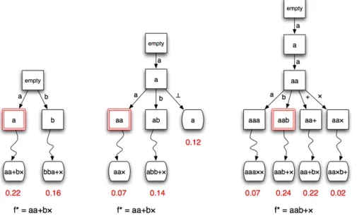
Fig. 2. Illustration of three steps of Algorithm 2 with the look-ahead strategy. Boxes denote states, curved edges denote random simulations and rounded boxes denote final states, i.e. constructed and evaluated features. Double-circled boxes denote the symbols of the best discovered feature so-far that are selected by the algorithm. Note that at the second step, the best discovered feature is still [a, a, +, b, ×], hence the selected symbol is a.
iteration d, the step strategy completes the current subsequence randomly and evaluates the corresponding feature. It then selects its next symbol as the d-th symbol of d-the currently best found feature f∗. Strategy look-ahead proceeds similarly, but makes more random simulations: one simulation per candidate successor symbol. This strategy corresponds to the level 1 nested Monte Carlo search algorithm [3]. Whatever the search strategy, our top-level algorithms work by repeatedly running the random, step or look-ahead strategy until K different features have been evaluated, i.e. search is stopped as soon as the split score function has been called K times. It then returns the best found feature.
Figure 2 illustrates three steps of our feature generation algorithm using the look-ahead strategy in a simple case with two input properties a and b and two constructor functions + and ×.
5
Experimental results
We validate our approach by embedding feature generation into five well-known classification algorithms: single trees, random forests, extremely randomized trees, boosted stumps and boosted trees. We focus on a set of 12 standard classification datasets, study the effect of the parameters D and K and compare algorithms embedding feature generation with their classical counter-parts.
5.1 Datasets and methods
We use the same set of 12 multi-class classification datasets as the authors of [7]. These well-known and publicy available datasets cover a wide range of conditions in terms of number of candidate attributes, presence of noise, non-linearity, ob-servation redundancy and irrelevant variables. We also use the same train/test splits and the same evaluation protocol as [7]: for each dataset and each algo-rithm, we measure the test classification error averaged over 50 train/test splits for the smaller datasets and 10 train/test splits for the larger datasets.
We embed feature generation into the following algorithms. Single trees (ST) are classical decision trees without pruning. Random forests (RF) [1] and ex-tremely randomized trees (ET) [7] are well-known ensemble methods. Boosted stumps (BS) and boosted decision trees (BT) rely on the AdaBoost.MH algo-rithm for multi-class classification [17]. For the ST, RF and ET methods, we use the information gain normalized in the same way as [7]. As in [9], when splitting nodes into boosted decision trees, we do not maximize information gain but rather directly maximize the edge, the objective of the weak learner in AdaBoost.MH.
Although our formalism enables to deal with input properties and constructor functions of different types, we focus here on a simpler case: all input proper-ties are numerical attributes and we construct features by using only the four mathematical operations +, ×, −, /. Applying our approach to more complex situations is left for future work.
5.2 Impact of parameters K and D
Our first series of experiments aims at studying the impact of the optimization budget K and the maximal feature size D on the performance of single trees, extremely randomized trees and boosted stumps. To study the impact of K, we choose a constant value D = 5, which for example enables to construct features such as a + b × c and vary K from 0.1n to 100n. We then set K to a constant value (either K = 100n for single trees or K = 10n for the other methods) and vary the maximal feature length D from 1 to 15.
Single trees. Figure 3 reports the results for single trees. The baseline corre-sponds to classical decision trees learned on the original variables of the prob-lem. First, we observe that feature generation does not systematically lead to improved decision trees, which was already observed in previous work on feature generation. Second, we observe that scores continuously get better when the optimization budget K is increased. This is in agreement with the traditional approach to feature generation involving computationally intensive search al-gorithms such as genetic programming. Since there is a single chance to build a good-performing tree (there is no ensemble effect), as much computational power as possible should be dedicated to feature search. There is no clear ten-dency concerning the parameter D, although we see that D = 5 seems to be a reasonable default value. The look-ahead strategy slightly outperforms the two other search strategies, although the overall difference is rather small.
10-1 100 101 102 15 20 25 30 35 40 classification error
vowel
102-1 100 101 102 46 8 10 12 14 1618 20segment
108-1 100 101 102 9 1011 12 13 14 15spambase
Baseline Random Step Look-ahead 10-1 100 101 102 K / n 14.014.5 15.015.5 16.016.5 17.0 classification errorsatellite
10-1 100 101 102 K / n 2 46 8 10 12 14pendigits
10-1 100 101 102 K / n 12 14 16 18 20 22 24 26 28 30dig44
(a) Impact of parameter K with D = 5
2 4 6 8 10 12 14 17.5 18.018.5 19.019.5 20.0 20.5 21.0 21.5 classification error
vowel
2 4 6 8 10 12 14 3.0 3.2 3.4 3.6 3.8 4.0segment
2 4 6 8 10 12 14 8 9 1011 12 13 14 15spambase
Baseline Random Step Look-ahead 2 4 6 8 10 12 14 D 13.8 14.014.2 14.4 14.6 14.8 15.015.2 classification errorsatellite
2 4 6 8 10 12 14 D 2.8 3.03.2 3.4 3.63.8 4.0pendigits
2 4 6 8 10 12 14 D 11.5 12.0 12.5 13.0 13.5 14.0 14.5 15.0dig44
(b) Impact of parameter D with K = 100n Fig. 3. Single trees
Extremely randomized trees. Figure 4 displays the results for ensembles of 100 extremely randomized trees. Our approaches are compared against traditional extremely randomized trees with parameter K tuned to give the best test scores. As previously, feature generation enables to obtain significantly improved mod-els on only a part of the datasets. On the four first datasets, the best scores are obtained for values of K ranging from 0.1n to 10n. As discussed in Section 3, extremely randomized trees (and random forests) rely on random subspaces to introduce randomization, which has been shown to lead to more robust ensem-ble models. We observe that, when extending these algorithms with automatic feature generation, it is still interesting to use random subspaces, i.e. to ex-plore a very small portion of the whole feature space at each node split. This phenomenon is particularly clear on the vowel dataset, for which we observe that investing too much computational power into feature search is
counter-10-1 100 101 102 1.2 1.4 1.6 1.8 2.0 2.2 2.4 2.6 2.8 classification error
vowel
10-1 100 101 102 1.0 1.5 2.0 2.5 3.0 3.5segment
10-1 100 101 102 4.0 4.5 5.0 5.5 6.0 6.5 7.0spambase
Baseline Random Step Look-ahead 10-1 100 101 102 K / n 7.8 8.0 8.2 8.48.6 8.8 9.0 9.2 classification errorsatellite
10-1 100 101 102 K / n 0.4 0.6 0.81.0 1.2 1.4 1.6 1.8 2.0pendigits
10-1 100 101 102 K / n 4.0 4.5 5.0 5.5 6.0 6.5 7.07.5dig44
(a) Impact of parameter K with D = 5
2 4 6 8 10 12 14 1.3 1.4 1.5 1.6 1.7 1.8 1.9 2.0 2.1 classification error
vowel
2 4 6 8 10 12 14 1.36 1.38 1.401.42 1.44 1.46 1.48 1.501.52segment
2 4 6 8 10 12 14 4.0 4.5 5.0 5.5 6.0 6.5 7.0spambase
Baseline Random Step Look-ahead 2 4 6 8 10 12 14 D 7.7 7.8 7.9 8.0 8.1 8.2 8.3 8.4 classification errorsatellite
2 4 6 8 10 12 14 D 0.45 0.50 0.55 0.60 0.65 0.70 0.75 0.80 0.85 0.90pendigits
2 4 6 8 10 12 14 D 4.0 4.2 4.4 4.6 4.8 5.05.2 5.4 5.6dig44
(b) Impact of parameter D with K = 10n Fig. 4. Extremely randomized trees
productive. On the three last datasets, our approach seems to work the best for small generated features of size D = 3. Again, there is very little difference between the three search strategies.
Boosted stumps. Figure 5 presents the results for ensembles of 1000 boosted stumps. We now observe that models with feature generation strongly outper-form classical boosted stumps on all datasets. We believe that this is mainly explained by the fact that the baseline model is not able to exploit multi-variate correlations, whereas our extended version can exploit multiple variables together thanks to generated features. The most impressive in these results is that, even with very small computational budgets K = 0.1n that correspond to testing one or a few features at each iteration, feature generation still yields significantly improved models. Furthermore, we observe that increasing K beyond 10n only
102-1 100 101 102 4 6 8 10 12 14 16 18 classification error
vowel
10-1 100 101 102 1.4 1.6 1.8 2.02.2 2.4 2.6segment
10-1 100 101 102 4.8 5.0 5.2 5.4 5.6spambase
Baseline Random Step Look-ahead 10-1 100 101 102 K / n 8.5 9.0 9.5 10.010.5 11.011.5 classification errorsatellite
10-1 100 101 102 K / n 0.00.5 1.0 1.5 2.02.5 3.0pendigits
10-1 100 101 102 K / n 3 45 67 8 9dig44
(a) Impact of parameter K with D = 5
2 4 6 8 10 12 14 2 4 6 8 10 12 14 16 18 classification error
vowel
2 4 6 8 10 12 14 1.2 1.4 1.6 1.8 2.02.2 2.4 2.6segment
2 4 6 8 10 12 14 4.5 5.0 5.5 6.0 6.5spambase
Baseline Random Step Look-ahead 2 4 6 8 10 12 14 D 8.5 9.0 9.5 10.010.5 11.011.5 classification errorsatellite
2 4 6 8 10 12 14 D 0.00.5 1.0 1.5 2.02.5 3.0pendigits
2 4 6 8 10 12 14 D 3 45 67 8 9dig44
(b) Impact of parameter D with K = 10n Fig. 5. Boosted stumps
brings slight or no improvements on the error. In these cases, there is thus no need to invest a huge amount of computational power in feature search to benefit from feature generation. We also observe that the method is here rather robust w.r.t. the choice of parameter D and again that differences between the three search strategies are small.
5.3 Overall comparison of methods
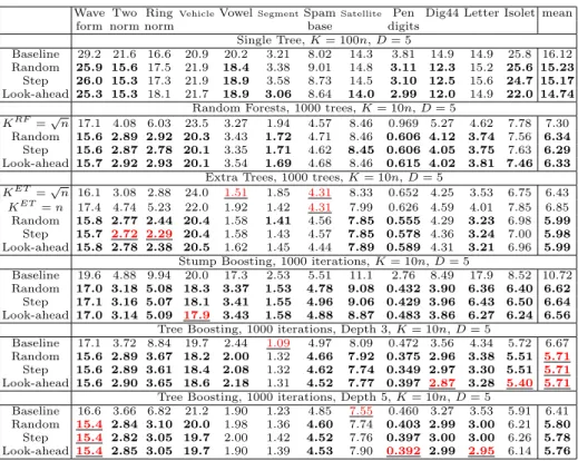
The results of embedding feature generation with our three search strategies into our five supervised learning algorithms are given in Table 3 for all our 12 datasets. For all methods, we use default settings for hyper-parameters: the maximal feature size is set to D = 5 in all cases, the feature search budget is set to K = 100n for single trees and K = 10n for ensemble models. The
Wave Two RingVehicleVowelSegmentSpamSatellite Pen Dig44 Letter Isolet mean
form norm norm base digits
Single Tree, K = 100n, D = 5
Baseline 29.2 21.6 16.6 20.9 20.2 3.21 8.02 14.3 3.81 14.9 14.9 25.8 16.12
Random 25.9 15.6 17.5 21.9 18.4 3.38 9.01 14.8 3.11 12.3 15.2 25.6 15.23
Step 26.0 15.3 17.3 21.9 18.9 3.58 8.73 14.5 3.10 12.5 15.6 24.7 15.17
Look-ahead 25.3 15.3 18.1 21.7 18.9 3.06 8.64 14.0 2.99 12.0 14.9 22.0 14.74
Random Forests, 1000 trees, K = 10n, D = 5
KRF =√n 17.1 4.08 6.03 23.5 3.27 1.94 4.57 8.46 0.969 5.27 4.62 7.78 7.30
Random 15.6 2.89 2.92 20.3 3.43 1.72 4.71 8.46 0.606 4.12 3.74 7.56 6.34
Step 15.6 2.87 2.78 20.1 3.35 1.71 4.62 8.45 0.606 4.05 3.75 7.63 6.29
Look-ahead 15.7 2.92 2.93 20.1 3.54 1.69 4.68 8.46 0.615 4.02 3.81 7.46 6.33
Extra Trees, 1000 trees, K = 10n, D = 5
KET =√n 16.1 3.08 2.88 24.0 1.51 1.85 4.31 8.33 0.652 4.25 3.53 6.75 6.43
KET = n 17.4 4.74 5.23 22.0 1.92 1.42 4.31 7.99 0.626 4.59 4.01 7.85 6.85
Random 15.8 2.77 2.44 20.4 1.58 1.41 4.56 7.85 0.555 4.29 3.23 6.98 5.99
Step 15.7 2.72 2.29 20.4 1.58 1.43 4.57 7.85 0.578 4.36 3.24 7.00 5.98
Look-ahead 15.8 2.78 2.38 20.5 1.62 1.45 4.44 7.89 0.589 4.31 3.21 6.96 5.99
Stump Boosting, 1000 iterations, K = 10n, D = 5
Baseline 19.6 4.88 9.94 20.0 17.3 2.53 5.51 11.1 2.76 8.49 17.9 8.52 10.72
Random 17.0 3.18 5.08 18.3 3.37 1.53 4.78 9.08 0.432 3.90 6.36 6.40 6.62
Step 17.1 3.16 5.07 18.1 3.41 1.55 4.96 9.06 0.429 3.96 6.43 6.50 6.64
Look-ahead 17.0 3.14 5.09 17.9 3.43 1.58 4.88 8.87 0.483 3.86 6.27 6.24 6.56
Tree Boosting, 1000 iterations, Depth 3, K = 10n, D = 5
Baseline 17.1 3.72 8.84 19.7 2.44 1.09 4.97 8.09 0.472 3.56 4.34 5.72 6.67
Random 15.6 2.89 3.67 18.2 2.00 1.32 4.66 7.92 0.375 2.96 3.38 5.51 5.71
Step 15.6 2.89 3.61 18.4 2.08 1.32 4.62 7.74 0.349 2.97 3.30 5.51 5.71
Look-ahead 15.6 2.90 3.65 18.6 2.18 1.31 4.52 7.77 0.397 2.87 3.28 5.40 5.71
Tree Boosting, 1000 iterations, Depth 5, K = 10n, D = 5
Baseline 16.6 3.66 6.82 21.2 1.90 1.23 4.85 7.55 0.460 3.27 3.53 5.91 6.41
Random 15.4 2.84 3.10 20.0 1.98 1.36 4.60 7.74 0.403 2.99 3.00 6.21 5.80
Step 15.4 2.82 3.05 19.7 2.00 1.42 4.52 7.76 0.397 3.00 3.00 6.26 5.78
Look-ahead 15.4 2.85 3.05 19.7 1.90 1.39 4.53 7.90 0.392 2.99 2.95 6.14 5.76
Table 3. Comparison of all methods with and without embedded feature generation. The scores (error rates in %) of methods embedding feature generation are shown in bold whenever they outperform those of the corresponding baseline(s). The best scores for each dataset are underlined.
baseline random forests are constructed with KRF =√n tested attributes per constructed splits. For extremely randomized trees, we consider the same two default setups as in [7]: KET =√n and KET = n.
We observe that embedding the Monte Carlo feature generation improves over the baselines about two times out of three, and on the average all methods are significantly improved thanks to the feature generation. Among the vari-ants we tested, the overall best scores are obtained when embedding feature generation in boosted decision trees of depth 3. The strongest improvement is however observed for boosted stumps, where we believe that there is a combined bias and variance reduction effect obtained thanks to the randomized feature construction. The net result is that, on the average, combining stump boost-ing with feature generation becomes competitive with baseline boosted trees of depth 3 or 5. Finally, while the ensemble methods are well improved when using a rather small budget for the search of features (K= 10n), standard trees may be improved by using a quite larger search budget (K= 100n).
6
Conclusion
Automatic feature generation approaches are usually classified into filters and wrappers. This paper emphasizes a third category: embedded feature generation. We have proposed a general scheme to embed feature generation into tree-based learning algorithms and have discussed the particularities of feature generation in the context of ensemble methods. In this latter context, we argued that it could be unnecessary or even counter-productive to invest a too large amount of computational power into feature search and therefore proposed three simple Monte Carlo search approaches to at the same time weakly and efficiently ex-plore the feature space, the number of trials allowing to control search strength. Our empirical investigations confirmed this analysis and showed also that the embedding of feature generation allows to improve the accuracy over a wide range of methods and datasets, the strongest improvements being found in the context of boosting, where Monte Carlo feature generation allows to both reduce bias (in the context of stumps) and variance (in the context of all versions).
For future research, we suggest to revisit in the light of our findings the earlier work on oblique decision trees (see e.g. [12]), which may also be viewed as a kind of embedded feature generation. On the other hand, while we focused in this paper on accuracy improvement, we believe that embedded feature generation should also be studied in terms of its effects on model complexity (e.g. in terms of the speed of convergence of the ensemble methods) and on interpretability (e.g. in terms of the capability to detect variable interactions of interest). Another line of research would be to see how to port the embedded feature generation towards L1-based regularization of generalized additive models, by building on the parallels of these approaches with boosting.
The formalism presented in this paper is very general in that it enables to formulate embedded feature generation on top of all kinds of raw data structures, including functional signals such as audio and images, and graph structured or relational data more and more frequently found in current application domains (e.g. ranging from bio-informatics to web-mining or automatic game playing). While our experiments focused on constructing features based on raw vectors of simple numerical features, we believe that embedded feature generation has even greater potentials to learn with such complex real-world data structures.
Acknowledgements
This paper presents research results of the European excellence network PAS-CAL2 and of the Belgian Network BIOMAGNET, funded by the Interuniversity Attraction Poles Programme, initiated by the Belgian State, Science Policy Of-fice. The scientific responsibility rests with the authors.
References
2. R. Caruana and A. Niculescu-Mizil. An empirical comparison of supervised learn-ing algorithms. In Proceedlearn-ings of the 23rd international conference on Machine learning, ICML ’06, pages 161–168, New York, NY, USA, 2006. ACM.
3. T. Cazenave. Nested monte-carlo search. In Proceedings of the 21st International Joint Conference on Artificial Intelligence (IJCAI’09), pages 456–461, 2009. 4. G. Chaslot, S. Bakkes, I. Szita, and P. Spronck. Monte-carlo tree search: A new
framework for game ai. In Christian Darken and Michael Mateas, editors, Pro-ceedings of the Fourth Artificial Intelligence and Interactive Digital Entertainment Conference, 2008.
5. A. Ek´art and A. M´arkus. Using genetic programming and decision trees for gener-ating structural descriptions of four bar mechanisms. Artif. Intell. Eng. Des. Anal. Manuf., 17(3):205–220, June 2003.
6. P.G. Espejo, S. Ventura, and F. Herrera. A survey on the application of genetic programming to classification. Trans. Sys. Man Cyber Part C, 40(2):121–144, March 2010.
7. P. Geurts, D. Ernst, and L. Wehenkel. Extremely randomized trees. Machine Learning, 36(1):3–42, 2006.
8. H. Guo, L.B. Jack, and A.K. Nandi. Feature generation using genetic programming with application to fault classification. IEEE Transactions on Systems, Man, and Cybernetics, Part B, 35(1):89–99, 2005.
9. B. K´egl and R. Busa-Fekete. Boosting products of base classifiers. In Proceedings of the 26th Annual International Conference on Machine Learning, ICML ’09, pages 497–504, New York, NY, USA, 2009. ACM.
10. K. Krzysztof. Genetic programming-based construction of features for machine learning and knowledge discovery tasks. Genetic Programming and Evolvable Ma-chines, 3(4):329–343, December 2002.
11. S. Markovitch and D. Rosenstein. Feature generation using general constructor functions. Machine Learning, 49:59–98, 2002.
12. S.K. Murthy, S. Kasif, and S. Salzberg. A system for induction of oblique decision trrees. Journal of Artificial Intelligence Research, 2:1–32, 1994.
13. A.Y. Ng. Feature selection, L1 vs. L2 regularization, and rotational invariance. In Proceedings of the twenty-first international conference on Machine learning, ICML ’04, New York, NY, USA, 2004. ACM.
14. F. Pachet and P. Roy. Analytical features: a knowledge-based approach to audio feature generation. EURASIP J. Audio Speech Music Process., 2009:1–23, 2009. 15. G. Pagallo and D. Haussler. Boolean feature discovery in empirical learning.
Ma-chine Learning, 5(1):71–99, May 1990.
16. M.L. Raymer, W.F. Punch, E.D. Goodman, and L.A. Kuhn. Genetic programming for improved data mining: application to the biochemistry of protein interactions. In Proceedings of the First Annual Conference on Genetic Programming, GECCO ’96, pages 375–380, Cambridge, MA, USA, 1996. MIT Press.
17. R.E. Schapire and Y. Singer. Improved boosting algorithms using confidence-rated predictions. Machine Learning, 37(3):297–336, December 1999.
18. M.G. Smith and L. Bull. Genetic programming with a genetic algorithm for fea-ture construction and selection. Genetic Programming and Evolvable Machines, 6(3):265–281, September 2005.
19. D.-S. Yang, L. Rendell, and G. Blix. A scheme for feature construction and a comparison of empirical methods. In Proceedings of the Twelfth International Joint Conference on Artificial Intelligence, pages 699–704. Morgan Kaufmann, 1991.