Application of the Nested Rollout Policy Adaptation Algorithm to the Traveling Salesman Problem with Time Windows

Application of the Nested Rollout Policy

Adaptation Algorithm to the Traveling Salesman

Problem with Time Windows

Tristan Cazenave1 _{and Fabien Teytaud}1,2

1 _{LAMSADE, Universit´e Paris Dauphine, France,}

2 _{HEC Paris, CNRS, 1 rue de la Lib´eration 78351 Jouy-en-Josas, France}

Abstract. In this paper, we are interested in the minimization of the travel cost of the traveling salesman problem with time windows. In order to do this minimization we use a Nested Rollout Policy Adaptation (NRPA) algorithm. NRPA has multiple levels and maintains the best tour at each level. It consists in learning a rollout policy at each level. We also show how to improve the original algorithm with a modified rollout policy that helps NRPA to avoid time windows violations.

Keywords:Nested Monte-Carlo, Nested Rollout Policy Adaptation, Trav-eling Salesman Problem with Time Windows.

1

Introduction

In this paper we are interested in the minimization of the travel cost of the Traveling Salesman Problem with Time Windows. Recently, the use of a Nested Monte-Carlo algorithm (combined with expert knowledge and an evolutionary algorithm) gave good results on a set of state of the art problems [13]. However, as it has been pointed out by the authors, the effectiveness of the Nested Monte-Carlo algorithm decreases as the number of cities increases. When the number of cities is too large (greater than 30 for this set of problems), the algorithm is not able to find the state of the art solutions.

A natural extension to the work presented in [13], which consists in the application of the Nested Monte-Carlo algorithm on a set of Traveling Salesman Problems with Time Windows, is to study the efficiency of the Nested Rollout Policy Adaptation algorithm on the same set of problems.

In this work we study the use of a Nested Rollout Policy Adaptation al-gorithm on the Traveling Salesman Problem with Time Windows. The Nested Rollout Policy Adaptation algorithm has recently been introduced in [15], and provides good results, including records in Morpion Solitaire and crossword puz-zles.

rollouts with a domain-specific one, defined as a mixture of heuristics. These domain-specific heuristics are presented in Section 4.2.

The paper is organized as follows. Section 2 describes the Traveling Sales-man Problem with Time Windows, Section 3 presents the Nested Monte-Carlo algorithm (Section 3.1) and its application to the Traveling Salesman Problem with Time Windows (Section 3.2). Section 4 presents the Nested Rollout Policy Adaptation algorithm (Section 4.1) and its application to the Traveling Sales-man Problem with Time Windows (Section 4.2). Section 5 presents a set of experiments concerning the application of the Nested Rollout Policy Adaptation algorithm on the Traveling Salesman Problem with Time Windows.

2

The Traveling Salesman Problem with Time Windows

The Traveling Salesman Problem (TSP) is a famous logistic problem. Given a list of cities and their pairwise distances, the goal of the problem is to find the shortest possible path that visits each city only once. The path has to start and finish at a given depot. The TSP problem is NP-hard [8]. In this work, we are interested in a similar problem but more difficult, the Traveling Salesman Problem with Time Windows (TSPTW). In this version, a difficulty is added. Each city has to be visited within a given period of time.

A survey of efficient methods for solving the TSPTW can be found in [9]. Existing methods for solving the TSPTW are numerous. First, branch and bound methods were used [1, 3]. Later, dynamic programing based methods [5] and heuristics based algorithms [17, 7] have been proposed. More recently, methods based on constraint programming have been published [6, 10].

An algorithm based on the Nested Monte-Carlo Search algorithm has been proposed [13] and is summarized in Section 3.2.

The TSPTW can be defined as follow. Let G be an undirected complete graph. G = (N, A), where N = 0, 1, . . . , n corresponds to a set of nodes and A = N × N corresponds to the set of edges between the nodes. The node 0 corresponds to the depot. Each city is represented by the n other nodes. A cost function c : A → R is given and represents the distance between two cities. A solution to this problem is a sequence of nodes P = (p0, p1, . . . , pn) where p0= 0

and (p1, . . . , pn) is a permutation of [1, N ]. Set pn+1 = 0 (the path must finish

at the depot), then the goal is to minimize the function defined in Equation 1. cost(P ) =

n

X

k=0

c(apk, apk+1) (1)

As said previously, the TSPTW version is more difficult because each city i has to be visited in a time interval [ei, li]. This means that a city i has to

be visited before li. It is possible to visit a cite before ei, but in that case, the

new departure time becomes ei. Consequently, this case may be dangerous as

the departure time dpk from this node is dpk= max(rpk, epk).

In the TSPTW, the function to minimize is the same as for the TSP (Equa-tion 1), but a set of constraint is added and must be satisfied. Let us define Ω(P ) as the number of violated windows constraints by tour (P).

Two constraints are defined. The first constraint is to check that the arrival time is lower than the fixed time. Formally,

∀pk, rpk < lpk.

The second constraint is the minimization of the time lost by waiting at a city. Formally,

rpk+1= max(rpk, epk) + c(apk,pk+1).

With the algorithm used in this work, paths with violated constraints can be generated. As presented in [13] , a new score T cost(p) of a path p can be defined as follow:

T cost(p) = cost(p) + 106_∗Ω(p),

with, as defined previously, cost(p) the cost of the path p and Ω(p) the number of violated constraints. 106 _{is a constant chosen high enough so that the algorithm}

first optimizes the constraints.

The TSPTW is much harder than the TSP, consequently new algorithms have to be used for solving this problem.

In the next sections, we define two algorithms for solving the TSPTW. The first one, in Section 3, is the Nested Monte-Carlo algorithm from [13], and the second one, in Section 4, is the Nested Rollout Policy Adaptation algorithm, which is used in this work to solve the TSPTW. We eventually present results in Section 5.

3

The Nested Monte-Carlo Search algorithm

First, in Section 3.1 we present the Nested Monte-Carlo Search, and then in Section 3.2 the application done in [13] to the Traveling Salesman Problem with Time Windows.

3.1 Presentation of the algorithm

The basic idea of Nested Monte-Carlo Search (NMC) is to find a solution path of cities with the particularity that each city choice is based on the results of a lower level of the algorithm [2]. At level 1, the lower level search is simply a playout (i.e. each city is chosen randomly).

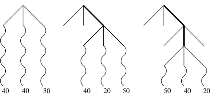
Figure 1 illustrates a level 1 Nested Monte-Carlo search. Three selections of cities at level 1 are shown. The leftmost tree shows that, at the root, all possible cities are tried and that for each possible decision a playout follows it. Among

the three possible cities at the root, the rightmost city has the best result of 30, therefore this is the first decision played at level 1. This brings us to the middle tree. After this first city choice, playouts are performed again for each possible city following the first choice. One of the cities has result 20 which is the best playout result among his siblings. So the algorithm continues with this decision as shown in the rightmost tree. This algorithm is presented in Algorithm 1.

Algorithm 1Nested Monte-Carlo search

nested (level,node) if level==0 then

ply ← 0 seq ← {}

whilenum children(node) > 0 do

CHOOSE seq[ply] ← child i with probability 1/num children(node) node ← child(node,seq[ply]) ply ← ply+1 end while RETURN (score(node),seq) else ply ← 0 seq ←{} best score ← ∞

whilenum children(node) > 0 do forchildren i of node do

temp ← child(node,i)

(results,new) ← nested(level-1,temp) if results<best score then

best score ← results seq[ply]=i seq[ply+1. . .]=new end if end for node=child(node,seq[ply]) ply←ply+1 end while

RETURN (best score,seq) end if

At each choice of a playout of level 1 it chooses the city that gives the best score when followed by a single random playout. Similarly for a playout of level nit chooses the city that gives the best score when followed by a playout of level n −1.

3.2 Application to the TSPTW

In [13], a NMC algorithm is used in order to solve a set of TSPTW. With the intention of having a competitive algorithm they add expert-knowledge to the

40 50 40

40 30 20 50 40 20

Fig. 1.This figure explains three steps of a level 1 search. At each step of the playout of level 1 shown here with a bold line, an NMC of level 1 performs a playout (shown with wavy lines) for each available decision and selects the best one.

NMC algorithm. Three heuristics are added and used to bias the Monte-Carlo simulations thanks to a Boltzmann softmax policy. The principle is to define a new policy for the rollout phase. This policy is defined by the probability πθ(p, a)

of choosing the action a in a position p: πθ(p, a) = eφ(p,a)T θ P beφ(p,b) T_θ,

where φ(p, a) is a vector of heuristics and θ is a vector of heuristic weights. The three heuristics used are the same as the ones defined in [17], and are summarised as follows:

– The distance to the last city.

– The amount of wasted time because a city is visited too-early. – The amount of time left until the end of the time window of a city.

For the tuning of the weights of each heuristic, they used an evolution strategy [12], more precisely a Self-Adaptive Evolution Strategy [12, 16], known for its robutsness.

4

The Nested Rollout Policy Adaptation algorithm

First, in Section 4.1, we present the Nested Rollout Policy Adaptation algorithm. In Section 4.2 we present some modifications done on this algorithm in order to improve it on the Traveling Salesman Problem with Time Windows.

4.1 Presentation of the Algorithm

The Nested Rollout Policy Adaptation algorithm (NRPA) is an algorithm that learns a playout policy. There are different levels in the algorithm. Each level is associated to the best sequence found at that level. The playout policy is a vector of weights that are used to calculate the probability of choosing a city. A city is chosen proportionally to exp(pol[code(node,i)]). pol(x) is the adaptable weight on code x. code(node,i) is a unique domain-specific integer leading from a situation node to its ith _{child. This is comparable with previous known}

learning of Monte-Carlo simulations [4, 14].

Learning the playout policy consists in increasing the weights associated to the best cities and decreasing the weights associated to the other cities. The algorithm is given in algorithm 2.

4.2 Application to the TSPTW

As for the NMC algorithm, adding expert-knowledge is possible in order to improve this generic algorithm. Consequently, the generality of the resulting algorithm is lower. We implement a NRPA algorithm with a specific Monte-Carlo policy.

The idea of this algorithm is first to force to visit cities as soon as they go after their window end. The reason is that cities that are after their window end should have been visited earlier and that must be taken into account for the continuation of the playout. If we force to visit them, the algorithm will try more to visit them in time.

The second idea of the algorithm is to avoid visiting a city if it makes another city go after its window end. It considers all the moves that do not make any city go after its window end.

These moves that avoid some cities can never be moves that force the algo-rithm into a suboptimal answer. These moves always imply a violation of the time window. Therefore they only change invalid solutions of the problem. An optimal move will not be pruned by our expert knowledge since it does not violate a constraint.

If there are still no possible moves after these two tests, the algorithm con-siders all the possible moves.

The resulting algorithm is labeled NRPA EK and is given in algorithm 3.

5

Experiments

First, in Section 5.1, we study the behaviour of the NRPA algorithm. Second, in Section 5.2, we compare it with the version defined in Section 4.2 on two problems among the set of problems from [11]. Finally, in Section 5.3, we provide a comparison of the two algorithms studied in this work, the NMC algorithm in [13] and the state of the art results found in [9].

Algorithm 2Nested Rollout Policy Adaptation NRPA (level,pol) if level= 0 then node← root ply← 0 seq← {}

whilethere are possible moves do

CHOOSE seq[ply] ← child i the with probability proportional to exp(pol[code(node,i)])

node← child(node, seq [ply]) ply←ply + 1

end while

return (score (node), seq) else

bestScore← ∞ forN iterations do

(result,new) ← NRPA (level − 1, pol) if result ≤ bestScore then

bestScore← result seq ← new end if pol← Adapt(pol,seq) end for end if return (bestScore,seq) Adapt (pol,seq) node← root pol′ _{← pol}

forply← 0 to length(seq) - 1 do pol′_{[code(node,seq[ply])] += Alpha}

z← SUM exp(pol[code(node,i)]) over node’s children i forchildren i of node do

pol′_{[code(node,i)] -= Alpha × exp(pol[code(node,i)]) / z}

end for

node← child(node, seq [ply]) end for

Algorithm 3Playout policy for NRPA EK

possibleMoves () s← {}

forall not yet visited cities c do

if going to the city c arrives after the window end of the city then add the city c to the set s

end if end for if s= {} then

forall not yet visited cities c do tooLate← false

forall not yet visited cities d different from c do

if going to the city d arrives before the window end of the city d and going to the city c arrives after the window end of the city d then

tooLate← true end if

end for

if not tooLate then add the city c to the set s end if

end for end if

if s= {} then

forall not yet visited cities c do add the city c to the set s end for

end if return s

5.1 The behaviour of the NRPA algorithm

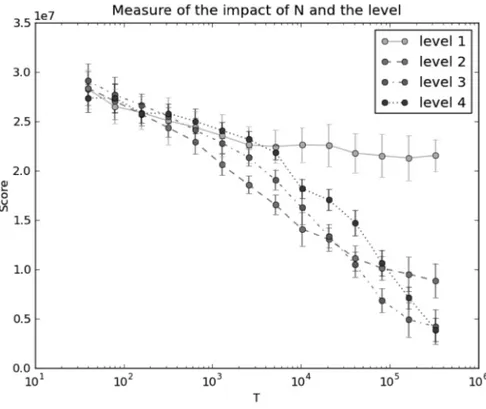
It has been found for the NMC algorithm and the NRPA algorithm (both on Morpion Solitaire) that a plateau is reached for each level of the algorithms, and then consequently, that increasing the level improves the results of the al-gorithms. In figure 2, similar results are shown for a TSPTW (on the problem rc204.1 from the set of problems from [11]). We measure the score of a NRPA algorithm as a function of the time T for different levels. The time T represents the number of evaluations done for each level. Formally, T = Nlevel_{. We recall}

that N is the number of iterations done for each level (> 0) of the NRPA algo-rithm. Each point is the average of 30 runs. Plateaus are here well represented. For the level 1, T = N , and we can note that increasing N beyond 1000 does not improve the algorithm. The level 2 of the NRPA algorithm is quickly better than a level 1. It is better to use the level 3 of the algorithm than the level 2 around T = 30000, this means, approximately for N = 170 for the level 2 and N = 30 for the level 3. The level 4 of the algorithm becomes better than the level 3 around T = 330000, so it corresponds to N = 575 for the level 3 and N = 70 for the level 4.

5.2 NRPA against NRPA EK

In this experiment we compare the NRPA algorithm (as defined in Algorithm 2) and the version of NRPA with expert knowledge, presented in Section 4.2. This last algorithm is labeled NRPA EK in all our experiments.

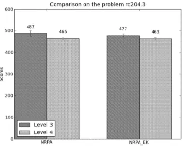
We test these two algorithms on two problems from the set of problems from [11], the problem rc204.3 and the problem rc204.1. This last problem is the hardest one among all the problems of the set, and has 46 cities. In all this experiment, N is fixed at 50. Results are presented in Figure 3 for the problem rc204.3 and in Figure 4 for the problem rc204.1.

Results of the rc204.3 problem (Figure 3) are close, because this problem is sim-ple enough for both algorithms and they are able to quickly find good solutions. However, the NRPA EK is slightly better for both the levels 3 and 4. On the hardest problem (Figure 4), results are much more significant. The level 3 of both the algorithms are not able to find a path with respect to all the time con-straints. In average, the NRPA EK version is able to solve one more constraint than the NRPA algorithm. For the level 4 comparison, the NRPA EK is by far better than the classic version of the algorithm and is able to find a path without any violated constraint in all the runs.

5.3 State Of The Art problems

We experiment the NRPA algorithm on all the problems from the set of [11]. Results are presented in Table 1. Problems are sorted according to n (i.e. the number of cities). The state of the art results are found by the ant colony al-gorithm from [9]. The fourth column represents the best score found in [13]. [13] uses an evolutionary algorithm for tuning heuristics used to bias the level

Fig. 2.Score as a function of T . Average on 30 runs. Plateaus are reached for the first three levels, and increasing the level of the algorithm improves the results.

Fig. 3.Comparison between the NRPA algorithm and the NRPA EK algorithm of the problem rc204.3. For both the algorithms N = 50.

Fig. 4.Comparison between the NRPA algorithm and the NRPA EK algorithm of the problem rc204.1. For both the algorithms N = 50.

0 of a Nested Monte-Carlo algorithm. The NRPA algorithm is somehow close to the NMC algorithm, and a comparison between these two algorithms on a set of TSPTW is interesting. The classic version of the NRPA algorithm does not use any expert knowledge, but is still able to achieve good results on a lot of problems (Table 1, fifth column). We provide the Relative Percentage Devia-tion (RPD) for both NRPA (column 6) and NRPA EK (column 8). The RPD is 100 × value - record

record . Here again, we show that adding expert knowledge is useful

and improves the algorithm. The NRPA EK version is able to find most state of the art results (76.66%), as shown in column 7. For difficult problems, the best results were obtained after 2 to 4 runs of the algorithm.

6

Conclusion

In this paper we study the generality of a nested rollout policy adaptation algo-rithm by applying it to traveling salesman problems with time windows. Even with no expert knowledge at all, the NRPA algorithm is able to find state of the art results for problems for which the number of nodes is not too large. We also experiment the addition of expert knowledge in this algorithm. With the good results of the algorithm NRPA EK, we show the feasability of guiding the rollout policy using domain-specific knowledge.

We show that adding expert knowledge significantly improves the results. It has been shown in our experiments that the NRPA EK algorithm (the expert knowledge version of the NRPA algorithm) is able to find most state of the art results (76.66%), and has good results on other problems.

An extension of this work is the use of a pool of policies (instead of just having one), in order to have an algorithm more robust in front of local optima. Adapting the parameters of the NRPA algorithm according to the problem difficulty is also an interesting work.

7

Acknowledgement

This work has been supported by French National Research Agency (ANR) through COSINUS program (project EXPLORA ANR-08-COSI-004)

References

1. E. Baker. An exact algorithm for the time-constrained traveling salesman problem. Operations Research, 31(5):938–945, 1983.

2. T. Cazenave. Nested Monte-Carlo search. In IJCAI, pages 456–461, 2009. 3. N. Christofides, A. Mingozzi, and P. Toth. State-space relaxation procedures for

the computation of bounds to routing problems. Networks, 11(2):145–164, 1981. 4. P. Drake. The last-good-reply policy for monte-carlo go. ICGA Journal, 32(4):221–

227, 2009.

5. Y. Dumas, J. Desrosiers, E. Gelinas, and M. Solomon. An optimal algorithm for the traveling salesman problem with time windows. Operations Research, 43(2):367– 371, 1995.

Problem n State of NMC NRPA RPD NRPA EK the art score score

rc206.1 4 117.85 117.85 117.85 0 117.85 0 rc207.4 6 119.64 119.64 119.64 0 119.64 0 rc202.2 14 304.14 304.14 304.14 0 304.14 0 rc205.1 14 343.21 343.21 343.21 0 343.21 0 rc203.4 15 314.29 314.29 314.29 0 314.29 0 rc203.1 19 453.48 453.48 453.48 0 453.48 0 rc201.1 20 444.54 444.54 444.54 0 444.54 0 rc204.3 24 455.03 455.03 455.03 0 455.03 0 rc206.3 25 574.42 574.42 574.42 0 574.42 0 rc201.2 26 711.54 711.54 711.54 0 711.54 0 rc201.4 26 793.64 793.64 793.64 0 793.64 0 rc205.2 27 755.93 755.93 755.93 0 755.93 0 rc202.4 28 793.03 793.03 800.18 0.90 793.03 0 rc205.4 28 760.47 760.47 765.38 0.65 760.47 0 rc202.3 29 837.72 837.72 839.58 0.22 839.58 0.22 rc208.2 29 533.78 536.04 537.74 0.74 533.78 0 rc207.2 31 701.25 707.74 702.17 0.13 701.25 0 rc201.3 32 790.61 790.61 796.98 0.81 790.61 0 rc204.2 33 662.16 675.33 673.89 1.77 664.38 0.34 rc202.1 33 771.78 776.47 775.59 0.49 772.18 0.05 rc203.2 33 784.16 784.16 784.16 0 784.16 0 rc207.3 33 682.40 687.58 688.50 0.83 682.40 0 rc207.1 34 732.68 743.29 743.72 1.51 738.74 0.83 rc205.3 35 825.06 828.27 828.36 0.40 825.06 0 rc208.3 36 634.44 641.17 656.40 3.46 650.49 2.53 rc203.3 37 817.53 837.72 820.93 0.42 817.53 0 rc206.2 37 828.06 839.18 829.07 0.12 828.06 0 rc206.4 38 831.67 859.07 831.72 0.01 831.67 0 rc208.1 38 789.25 797.89 799.24 1.27 793.60 0.55 rc204.1 46 868.76 899.79 883.85 1.74 880.89 1.40

Table 1. Results on all problems from the set from Potvin and Bengio [11]. First Column is the problem, second column the number of nodes, third column the best score found in [9], fourth column the best score found by the NMC algorithm with heuristics from [13], fifth column is the best score found by the NRPA algorithm and sixth column is its corresponding RPD. Seventh and eighth columns are respectively the score of the NRPA EK algorithm and the corresponding RPD. The problems for which we find the state of the art solutions are in bold.

6. F. Focacci, A. Lodi, and M. Milano. A hybrid exact algorithm for the tsptw. INFORMS Journal on Computing, 14(4):403–417, 2002.

7. M. Gendreau, A. Hertz, G. Laporte, and M. Stan. A generalized insertion heuris-tic for the traveling salesman problem with time windows. Operations Research, 46(3):330–335, 1998.

8. D. Johnson and C. Papadimitriou. Computational complexity and the traveling salesman problem. Mass. Inst. of Technology, Laboratory for Computer Science, 1981.

9. M. L´opez-Ib´a˜nez and C. Blum. Beam-ACO for the travelling salesman problem with time windows. Computers & OR, 37(9):1570–1583, 2010.

10. G. Pesant, M. Gendreau, J. Potvin, and J. Rousseau. An exact constraint logic programming algorithm for the traveling salesman problem with time windows. Transportation Science, 32(1):12–29, 1998.

11. J. Potvin and S. Bengio. The vehicle routing problem with time windows part II: genetic search. INFORMS journal on Computing, 8(2):165, 1996.

12. I. Rechenberg. Evolutionsstrategie: Optimierung technischer Systeme nach Prinzipien der biologischen Evolution, Fromman-Holzboog. Stuttgart. German, 1973.

13. A. Rimmel, F. Teytaud, and T. Cazenave. Optimization of the nested monte-carlo algorithm on the traveling salesman problem with time windows. Applications of Evolutionary Computation, pages 501–510, 2011.

14. A. Rimmel, F. Teytaud, and O. Teytaud. Biasing monte-carlo simulations through rave values. Computers and Games, pages 59–68, 2011.

15. C. D. Rosin. Nested rollout policy adaptation for monte carlo tree search. In T. Walsh, editor, IJCAI, pages 649–654. IJCAI/AAAI, 2011.

16. H. Schwefel. Adaptive Mechanismen in der biologischen Evolution und ihr Einfluß auf die Evolutionsgeschwindigkeit. Interner Bericht der Arbeitsgruppe Bionik und Evolutionstechnik am Institut f

”ur Mess-und Regelungstechnik Re, 215(3), 1974.

17. M. Solomon. Algorithms for the vehicle routing and scheduling problems with time window constraints. Operations Research, 35(2):254–265, 1987.