Cellular GPU Models to Euclidean Optimization Problems : Applications from Stereo Matching to Structured Adaptive Meshing and Traveling Salesman Problem

HAL Id: tel-00982405

https://tel.archives-ouvertes.fr/tel-00982405

HAL is a multi-disciplinary open access archive for the deposit and dissemination of sci-entific research documents, whether they are pub-lished or not. The documents may come from teaching and research institutions in France or abroad, or from public or private research centers.

L’archive ouverte pluridisciplinaire HAL, est destinée au dépôt et à la diffusion de documents scientifiques de niveau recherche, publiés ou non, émanant des établissements d’enseignement et de recherche français ou étrangers, des laboratoires publics ou privés.

Problems : Applications from Stereo Matching to

Structured Adaptive Meshing and Traveling Salesman

Problem

Naiyu Zhang

To cite this version:

Naiyu Zhang. Cellular GPU Models to Euclidean Optimization Problems : Applications from Stereo Matching to Structured Adaptive Meshing and Traveling Salesman Problem. Computers and Society [cs.CY]. Université de Technologie de Belfort-Montbeliard, 2013. English. �NNT : 2013BELF0215�. �tel-00982405�

n

é c o l e d o c t o r a l e _{s c i e n c e s p o u r l ’ i n g é n i e u r e t m i c r o t e c h n i q u e s}

U N I V E R S I T É D E T E C H N O L O G I E B E L F O R T - M O N T B É L I A R D

Cellular GPU Models to Euclidean

Optimization Problems

Applications from Stereo Matching to Structured Adaptive

Meshing and Travelling Salesman Problem

é c o l e d o c t o r a l e _{s c i e n c e s p o u r l ’ i n g é n i e u r e t m i c r o t e c h n i q u e s}

U N I V E R S I T É D E T E C H N O L O G I E B E L F O R T - M O N T B É L I A R D

TH `

ESE pr ´esent ´ee par

Naiyu

ZHANG

pour obtenir le

Grade de Docteur de

l’Universit ´e de Technologie de Belfort-Montb ´eliard

Cellular GPU Models to Euclidean Optimization

Problems

Applications from Stereo Matching to Structured Adaptive Meshing and

Travelling Salesman Problem

Soutenue le 2 D ´ecembre 2013 devant le Jury :

AbdelazizBENSRHAIR Rapporteur Professeur des Universit ´es `a l’Institut National des Sciences Appliqu ´ees de Rouen

Ren ´eSCHOTT Rapporteur Professeur des Universit ´es `a l’Universit ´e de Lorraine, Nancy

LhassaneIDOUMGHAR Examinateur Maˆıtre de Conf ´erences HDR `a l’Universit ´e de Haute Alsace

BehzadSHARIAT Examinateur Professeur des Universit ´es `a l’Universit ´e Claude Bernard de Lyon I

Jean-CharlesCREPUT Directeur Maˆıtre de Conf ´erences HDR `a l’Universit ´e de Technologie de Belfort-Montb ´eliard

Abderrafi ˆaaKOUKAM Examinateur Professeur des Universit ´es `a l’Universit ´e de Technologie de Belfort-Montb ´eliard

YassineRUICHEK Examinateur Professeur des Universit ´es `a l’Universit ´e de Technologie de Belfort-Montb ´eliard

At the final stage of preparing the documentation of my work, this section gives me the opportunity to express my gratitude to all the people who supported and assisted me. First of all, my research would not have been possible without the generous funding of CSC-China Scholarship Council programme1_.

1 General Introduction 13

1.1 Context . . . 13

1.2 Objectives and concern of this work . . . 13

1.3 Plan of the document . . . 15

I Background 17 2 Background on GPU computing 19 2.1 Introduction . . . 19

2.2 GPU architecture . . . 19

2.2.1 Hardware organization . . . 19

2.2.2 Memory system . . . 21

2.2.2.1 Memory hierarchy . . . 21

2.2.2.2 Coalesced and uncoalesced global memory accesses . . . 23

2.2.2.3 On-chip shared memory . . . 25

2.3 CUDA . . . 25

2.3.1 The CUDA programming model . . . 25

2.3.2 SPMD parallel programming paradigm . . . 27

2.3.3 Threads in CUDA . . . 28

2.3.4 Scalability . . . 28

2.3.5 Synchronization effects . . . 29

2.3.6 Warp divergence . . . 30

2.3.7 Execution configuration of blocks and grids . . . 30

2.4 Conclusion . . . 31

3 Background on stereo-matching problems 33 3.1 Introduction . . . 33

3.2 Definition of stereovision . . . 33

3.2.2 Order phenomenon . . . 36

3.3 Stereo matching methods . . . 36

3.3.1 Method classification . . . 36

3.3.2 Dense stereo-matching method . . . 37

3.3.3 Matching cost computation . . . 37

3.3.4 Window for cost aggregation . . . 39

3.3.5 Best correspondence decision . . . 39

3.3.6 Left-right consistency check . . . 40

3.4 Two implementations of stereo-matching problems . . . 42

3.4.1 Introduction to CFA stereo-matching problems . . . 42

3.4.2 Introduction to real-time stereo-matching methods . . . 42

3.5 Related works on stereo-matching problems . . . 43

3.5.1 Current progress in the real-time stereo computation . . . 43

3.5.2 Parallel computing based on GPU in stereo-matching . . . 45

3.6 Conclusion . . . 46

4 Background on self-organizing map and structured meshing problems 47 4.1 Introduction . . . 47

4.2 Self-organizing map for GPU structured meshing . . . 48

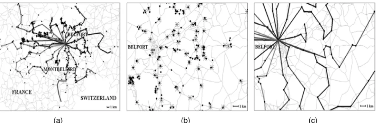
4.3 Adaptive meshing for transportation problems . . . 49

4.4 Parallel computing for Euclidean traveling salesman problem . . . 52

4.4.1 Solving TSPs on general parallel platforms . . . 52

4.4.2 Solving TSPs on GPU parallel platform . . . 53

4.5 Conclusion . . . 53

II Cellular GPU Model on Euclidean Optimization Problems 55 5 Parallel cellular model for Euclidean optimization problems 57 5.1 Introduction . . . 57

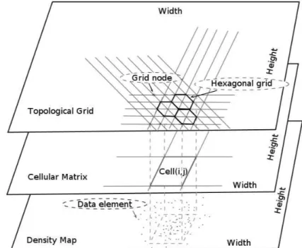
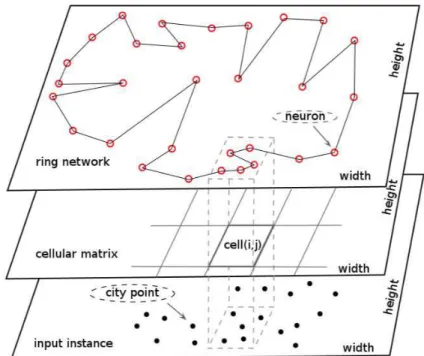
5.2 Data and treatment decomposition by cellular matrix . . . 58

5.3 Application to stereo-matching . . . 59

5.3.1 Local dense stereo-matching parallel model . . . 60

5.3.1.1 CFA stereo-matching application . . . 60

5.3.1.2 Real-time stereo-matching application . . . 61

5.4 Application to balanced structured meshing . . . 62

5.4.1 The self-organizing map algorithm . . . 62

5.4.2 The balanced structured mesh problem . . . 64

5.4.3 Euclidean traveling salesman problem . . . 66

5.4.4 Parallel cellular model . . . 66

5.4.4.1 Data treatment partition . . . 66

5.4.4.2 Thread activation and data point extraction . . . 68

5.4.4.3 Parallel spiral search and learning step . . . 70

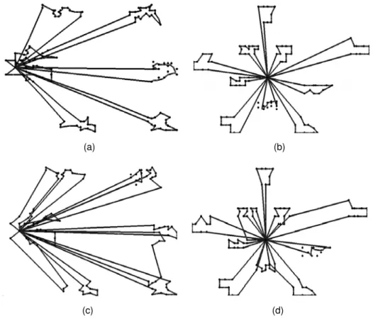
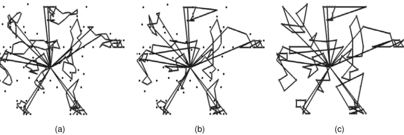
5.4.4.4 Examples of execution . . . 71

5.5 Conclusion . . . 72

6 GPU implementation of cellular stereo-matching agorithms 73 6.1 Introduction . . . 73

6.2 CFA demosaicing stereovision problem . . . 73

6.2.1 CFA demosaicing stereovision solution . . . 74

6.2.1.1 CFA stereovision process . . . 74

6.2.1.2 Second color component . . . 76

6.2.1.3 SCC estimation . . . 76 6.2.1.4 Matching cost . . . 77 6.2.2 Experiment . . . 77 6.2.2.1 Experiment platform . . . 77 6.2.2.2 CUDA implementation . . . 78 6.2.2.3 Experiment results . . . 80

6.3 Real-time stereo-matching problem . . . 83

6.3.1 Acceleration mechanisms and memory management . . . 83

6.3.2 Adaptive stereo-matching solution . . . 85

6.3.2.1 Matching cost . . . 85

6.3.2.2 Updated cost aggregation . . . 86

6.3.2.3 Simple refinement . . . 87

6.3.3 Experiment . . . 88

6.3.3.1 CUDA implementation . . . 88

6.3.3.2 Experiment results . . . 89

6.4 Conclusion . . . 94

7 GPU implementation of cellular meshing algorithms 97 7.1 Introduction . . . 97

7.2 GPU implementation of parallel SOM . . . 98

7.2.1 Platform background and memory management . . . 98

7.2.2 CUDA program flow . . . 98

7.2.3 Parallel SOM kernel . . . 100

7.3 Application to balanced structured mesh problem . . . 101

7.3.1 CUDA implementation specificities . . . 101

7.3.2 Experiments overview and parameters . . . 102

7.3.3 Experiments results . . . 103

7.4 Application to large scale Euclidean TSP . . . 107

7.4.1 Warp divergence analysis . . . 107

7.4.2 Experiments overview and parameters . . . 108

7.4.3 Comparative GPU/CPU results on large size TSP problems . . . 108

7.5 Conclusion . . . 110

III Conclusions and Perspectives 111 8 Conclusion 113 8.1 General conclusion . . . 113

8.2 Perspective and further research directions . . . 114

IV Appendix 117 A Input image pairs 119 A.1 Left image for CFA stereo matching . . . 119

A.2 Right image for CFA stereo matching . . . 119

A.3 Benchmark disparity for CFA stereo matching . . . 119

A.4 Input image pairs for real-time stereo matching . . . 119

B Experiment results 125 B.1 CFA stereo matching results on full size images . . . 125

B.2 CFA stereo matching results on half size images . . . 125

List of figures 125

List of tables 131

1

G

ENERAL

I

NTRODUCTION

1.1/

C

It is now a general tendency that computers integrate more and more transistors and processing units into a single chip. Personal computers are currently multi-core platforms. This happens in accordance with the Moore’s law that states that the number of transistors on integrated circuits doubles approximately every two years. At the same time, personal computers most often integrate graphic acceleration multiprocessor cards that become more and more cheaper. This is particularly true for Graphics Processing Units (GPU) which were originally hardware blocks optimized for a small set of graphics operations. Hence, the concept of GPGPU, that stands for general-purpose computing on graphics processing units, emerges by recognizing the trend of employing GPU technology for not only graphic applications but also general applications. In general, the graphic chips, due to their intrinsic nature of multi-core processors and being based on hundreds of floating-point specialized processing units, make many algorithms able to obtain higher performances than usual Central Processing Unit (CPU).

The main objective of this work is to propose parallel computation models and parallel algorithms that should benefit from the GPU’s enormous computational power. The focus is put on the field of combinatorial optimization and applications in embedded systems and terrestrial transportation systems. More precisely, we develop tools in relation to Euclidean optimization problems in both domains of stereovision image processing and routing problems in the plane. These problems are NP-hard optimization problems. This work presents and addresses stereo-matching problem, balanced structured meshing problem of a data distribution, and also the well known Euclidean traveling salesman problem. Specific GPU parallel computation models are presented and discussed.

1.2/

O

Propose a computation model for GPU that allows

(i) massive GPU parallel computation for Euclidean optimization problems, such as image processing and TSP,

(ii) application in real-time context and/or to large scale problems within acceptable computation time.

In the field of optimization, GPU implementations are more and more studied to ac-celerate metaheuristics methods to deal with NP-hard optimization problems, and large size problems that can not be addressed efficiently by exact methods. Here, we restrict our attention to heuristics and metaheuristics. Often, they exploit natural parallelism of metaphors, such as ant colony algorithms, or genetic algorithms that present an inherent level of parallelism by the use of a pool of solutions to which can be applied simultaneous independent operations. A most studied example, is the computation of solution evalua-tions in a parallel way. Meanwhile, such methods are based on parallel duplication of the solution data for parallelism. According to a fixed memory size GPU device, it follows that the input problem data size should decrease with the increase of the population size, and hence with the increase of the number processing units used in parallel. Such popula-tion based approach is memory consuming if one wants to deal with large size problems and large size populations together, that are contradictory requirements. Other methods are local search or neighborhood search approaches that operate on a single solution by improving it, successively with a neighborhood search operator. In that case, most of the GPU approaches try to compute the neighborhood candidates in parallel and select the best candidate. Due to the size of neighborhoods which are generally large, such approaches are facing to a difficult implementation problem of GPU resources manage-ment. The number of threads could be very high. For example, a single 2-opt improve-ment move should require O(N2) evaluations, with N the problem size. How to assign such evaluations computation to parallel threads is a difficult question. For the moment of writing, it looks that such approaches have only addressed relatively small size problems, considering a very standard problem such as the Euclidean traveling salesman problem. For each problem at hand, the designer has to carefully assign neighborhood operations to computation resources, as threads and registers.

To contribute at the development of GPU approaches able to deal with large size prob-lems, we restrict our attention to Euclidean optimization problems and address a different way to tackle data input at a low level of granularity. We follow the local dense approaches in image processing that simply assign a little part of the data to each computing unit. Pix-els of an image constitute a cellular decomposition of the data that yields to a natural level of computational parallelism. To address different Euclidean optimization problems, we extend the model of cellular decomposition to neural networks topological map algorithms that operate by the multiplication of simple operations in the plane. Such operations pro-duce, or make emerge, the required solution. The general approach that we retain for massive parallelism computation is cellular decomposition of the plane between a grid of cells, each one assigned to a given small and constant part of the input data, and hence to a single processing unit.

The cellular decomposition concerns input data of the problem. The approach differs from cellular genetic algorithms where processors are organized into a grid and where each one manages an independent solution. Such approach exploits data duplication parallelism, whereas our approach exploits data decomposition parallelism. An important

point, is that we are using such decomposition in accordance to the problem size, with a linear relationship, in order to address large size problems. We will illustrate that point on the Euclidean traveling salesman problem. Another point, is that we focus on a distributed and decentralized algorithm, with quite no intervention of the CPU during computation. It is worth noting that GPU local search methods often operate in a sequential/parallel way, where CPU may have a central role to prepare the next parallel computation for neighbor-hood move. We only consider methods where no solution transfers occurs between GPU and CPU during the course of the parallel execution. The main points are a low granu-larity level of data decomposition, together with distributed computation with no central control. The parallel cellular model does not prevent from using it into larger population based methods, or in combination with standard local search operators. We are inves-tigating a complementary way of addressing some Euclidean optimization problems that can be embedded in more general strategies.

In this work, we are implementing two types of algorithms. They are the winner-takes-all (WTA) local dense algorithm for stereo-matching and the self-organizing map (SOM) neu-ral network algorithm for structured meshing. The continuity of the method is illustrated on applications in the field of artificial vision, 3D surface reconstruction, that use both methods, and to Euclidean traveling salesman problem that uses the SOM.

The goal of a stereo-matching algorithm is to produce a disparity map that represents the 3D surface reconstructed from an image pair acquired by a stereo camera. We first study a stereo-matching method based on color filter array (CFA) image pairs. If a naive and direct GPU implementation can easily accelerate its CPU counterpart, the real-time requirement could be achieved. Then, starting from this basic GPU application, we investigate acceleration mechanisms to allow near real-time computation. Memory management appears to be a central factor for computation acceleration, whereas use of specific support region for matching and refinement steps improve quality substantially. Then, the parallel self-organizing map for compressed structured mesh generation is pre-sented. Starting from a disparity map as input, the algorithm generates an hexagonal mesh that can be used as a compressed representation of the 3D surface, with improved details for the objects of the scene nearest to the camera. By using the same algorithm, we address the traveling salesman problem and large size instances with up to 33708 cities. For SOM applications, a basic characteristic is the many spiral search of closest points in the plane, each one performed in time complexity O(1), in average when dealing with a bounded data distribution. Then, one of the main interests of the proposed ap-proach is to allow the execution of approximately N spiral searches in parallel, where N is the problem size. This is what we call “massive parallelism”, the theoretical possibility to reduce average computation time by factor N, and many repetitions of constant time simple operations. We systematically study the influence of problem size, together with the trade-off between solution quality and computation time on both CPU and GPU, in order to gauge the benefit of massive parallelism.

1.3/

P

According to the objectives and concerns, this thesis is organized into two main parts: one part is related to background definitions and exposition of state-of-the-art methods, the other part is devoted to the proposed model, solution approaches and experiments. The plan is summarized in Fig. 1.1.

Figure 1.1: Reading directions

The first part is composed of chapters 2, 3, and 4. Chapter 2 presents the GPU compu-tation architecture and its related CUDA programming model. Chapter 3 presents back-ground on stereovision, and reviews local dense stereo-matching method already applied on CPU and GPU plateforms. Chapter 4 presents background on the self-organizing map and of its application on structured meshing and transportation problems. For each ap-plication and algorithm, these chapters try to present the state-of-the-art in parallel GPU computing for such problems.

The second part of the document is composed of chapters 5, 6, and 7. Chapter 5 presents the cellular GPU parallel model for massive parallel computation for Euclidean optimiza-tion problems. Chapter 6 presents applicaoptimiza-tion to stereo-matching problems for CFA de-mosaicing stereovision and the real-time stereo-matching implementation that is derived from the standard local dense scheme. Chapter 7 presents details about the two GPU applications of the cellular parallel SOM algorithm. The two applications are the balanced structured mesh problem applied on disparity map, and the well-known Euclidean travel-ing salesman optimization problem.

Then, a general conclusion finishes the document. A section specially exposes the per-spectives of this work for parallel optimization computation in the future.

I

2

B

ACKGROUND ON

GPU

COMPUTING

2.1/

I

Most personal computers can now integrate GPU cards at very low cost. That is the reason why it would be very interesting to exploit this enormous capability of computing to implement parallel models for optimization applications. In this chapter, we will introduce the background of the GPU architecture and the CUDA programming environment used in our work. Specifically, we will first present the GPU hardware organization and memory system. Then we will give general introductions to the CUDA programming model and the Single-Program Multiple-Data (SPMD) parallel programming paradigm, explain the thread and memory management, outline the scalability and synchronization effects of this model, and introduce the configuration of block and grid in multi-thread execution.

2.2/

GPU

In this section, we provide a brief background on the GPU architecture. Our analytical model is based on the Compute Unified Device Architecture (CUDA) programming model and the NVIDIA Fermi architecture [GTX13] used in the GeForce GTX 570 GPU.

2.2.1/ HARDWARE ORGANIZATION

For years, the use of graphics processors was dedicated to graphics applications. Driven by the demand for high-definition 3D graphics on personal computers, GPUs have evolved into a highly parallel, multi-threaded and many-core environment. Indeed, this architec-ture provides a tremendous powerful computational capability and a very high memory bandwidth compared to traditional CPUs. The repartition of transistors between the two architectures can be illustrated as Fig. 2.1.

We can see in Fig. 2.1 that CPU does not have a lot of Arithmetic-Logic Units (ALU in the figure), but a large cache and an important control unit. And therefore, CPU is specialized for management of multiple and different tasks in parallel that require lots of data. In this case, data are stored within a cache to accelerate its accesses. While the control unit will handle the instructions flow to maximize the occupation of ALU, and to optimize the cache management. In other hand, GPU has a large number of arithmetic units with limited cache and few control units. This architecture allows the GPU to compute in a massive and parallel way the rendering of small and independent elements, while having a large flow of data processed. Since in GPU, more transistors are devoted to data processing rather than data caching and flow control, GPU is specialized for intensive and highly parallel computations.

Figure 2.2: A sketch map of GPU architecture.

Fig. 2.2 provides a display of the global GPU architecture. The GPU architecture consists of a scalable number of streaming multiprocessors (SMs). For GTX 570, the number of SM is 15, and each SM features 32 single-precision streaming processors (SPs), which are more usually called CUDA cores, four special function units (SFUs) executing tran-scendental instructions such as sin, cos, reciprocal and square root. Each SFU executes one instruction per thread per clock and a warp executes over eight clocks. A 64KB high speed on-chip memory (Shared Memory/L1 Cache) and an interface to a second cache are also equipped for each SM [Gla13].

instruc-tion consists of applying the instrucinstruc-tion to 32 threads. In the Fermi architecture a warp is formed with a batch of 32 threads. The GPU of the Fermi architecture uses a two-level, distributed thread scheduler for warp scheduling. The GigaThread Engine is above the SM level and the Dual warp Scheduler at the SM level, the later is the one more usually concerned. Each SM can issue instructions consuming any two of the four blue execu-tion columns shown in Fig. 2.2. For example, the SM can mix 16 operaexecu-tions from the 16 cores in the first column with 16 operations from the 16 cores in the second two-column or 16 operations from the load/store units or any other combinations the program specifies. Normally speaking, one SM can issue up to 32 single-precision (32-bit) floating point operations or 16 double-precision (64-bit) floating point operations at a time. More precisely, at the SM level, each warp scheduler distributes warps of 32 threads to its exe-cution units. Threads are scheduled in warp. Each SM features two warp schedulers and two instruction dispatch units, allowing two warps to be issued and executed concurrently. The dual warp scheduler selects two warps and issues one instruction from each warp to a group of 16 cores, 16 load/store (shown as the L/S units in Fig. 2.2 ) units or 4 SFUs. Most instructions can be dually issued, such as two integer instructions, two floating in-structions or a mix of integer, floating point. Load, store and SFU inin-structions can be issued concurrently also. Double precision instructions do not support dual dispatch with any other operations.

2.2.2/ MEMORY SYSTEM

2.2.2.1/ MEMORY HIERARCHY

From a hardware point of view, GPU consists of streaming multiprocessors, each with processing units, registers and on-chip memory. As multiprocessors are organized ac-cording to the SPMD model, threads share the same code and have access to different memory space. Table 2.1 and Fig. 2.3 show these different available memory space and connections with threads and blocks.

Table 2.1: GPU MEMORY SPACE. Memory Type Access Latency Size

Global Medium Large

Registers Very fast Very small

Local Medium Medium

Shared Fast Small

Constant Fast (cached) Medium Texture Fast (cached) Medium

The communication between CPU and GPU is done through the global memory. How-ever, in most GPU configurations, this memory is not cached and its access is quite slow, people have to minimize accesses to global memory for both read/write operations and reuse data within the local multiprocessor memory space. GPU has also read-only tex-ture memory to accelerate operations such as 2D and 3D mapping. Textex-ture memory space can be used for fast graphic operations. It is usually used by binding texture on global memory. Indeed, it can improve random accesses or uncoalesced memory ac-cess patterns that occur in common applications. Constant memory is another read-only

memory, but its hardware is optimized for the case where all threads read the same lo-cation. Shared memory is a fast memory located on the multiprocessors and shared by threads of each thread block. This memory area provides a way for threads to commu-nicate within the same block. Registers among streaming processors are exclusive to an individual thread; they constitute a fast access memory. In a kernel code, that is a global CUDA funtion, each declared variable is automatically put into registers. Local memory is a memory abstraction and is not an actual hardware component. In fact, local mem-ory resides in the global memmem-ory allocated by the compiler. Complex structures such as declared arrays will reside in local memory. In addition, the local memory is meant as a memory location used to hold “spilled” registers. Register spilling occurs when a thread block requires more registers than available ones on an SM. Local memory is used only for some automatic variables, which are declared in the device code without any of the qualifiers, such as device , shared , or constant . Generally, an automatic vari-able resides in a register except for the following cases: arrays that the compiler cannot determine are indexed with constant quantities and large structures or arrays that would consume too much register space. Any variable can be spilled by the compiler to local memory, when a kernel uses more registers than that are available on the SM.

2.2.2.2/ COALESCED AND UNCOALESCED GLOBAL MEMORY ACCESSES

Regarding the executing processing, the SM processor executes one warp at one time and schedules warps in a time-sharing fashion. The processor has enough functional units and register read/write ports to execute 32 threads together. When the SM pro-cessor executes a memory instruction1, it generates memory requests and switches to another warp until all the memory values in the warp are ready. Ideally, all the memory accesses within a warp can be combined into one memory transaction. In fact, for best performance, accesses by threads in a warp must be coalesced into a single memory transaction of 32, 64 or 128 bytes. Unfortunately, that depends on the memory access pattern within a warp. If the memory addresses are sequential, all of the memory re-quests within a warp can be coalesced into a single memory transaction. Otherwise, each memory address will generate a different transaction. Fig. 2.4 illustrates two exam-ples for each of these two cases. The CUDA manual [NVI10] provides detailed algorithms to identify types of coalesced/uncoalesced memory accesses. If memory requests in a warp are uncoalesced, the warp cannot be executed until all the memory transactions from the same warp are serviced, which will take significantly longer time than waiting for only one memory request as in the coalesced case and it can lead to a significantly per-formance decrease. However, some modifications have been done as a solution to the problem of latency in the case of uncoalesced memory accesses. Generally speaking, before the GPU compute capability version 1.3, stricter rules are applied to be coalesced. When memory requests are uncoalesced, one warp generates 32 memory transactions. While in the later versions after version 1.3, the rules are more relaxed and all memory requests are coalesced into as few memory transactions as possible [HK09].

(a)Example 1 1: Coalesced float memory ac-cess resulting in single memory transaction.

(b) Example 1 2: Coalesced float memory ac-cess ( divergent warp ) resulting in single mem-ory transaction.

(c) Example 2 1: Non-sequential float mem-ory access resulting in sixteen memmem-ory trans-actions.

(d) Example 2 2: Access with misaligned starting address float, resulting in sixteen memory transactions.

2.2.2.3/ ON-CHIP SHARED MEMORY

While the global memory is part of the off-chip Dynamic Random Access Memory (DRAM), the shared memory is implemented within each SM multiprocessor as a Static Random Access Memory (SRAM). The shared memory has very low access latency, which is almost the same as that of register, normally 10-20 cycle, and high bandwidth of 1,600 GB/s, which has been widely investigated to reduce non-coalesced global memory accesses in regular applications [SRS+_{08]. However, since one warp of 32 threads} ac-cesses the shared memory together, when there is a bank conflict within a warp, access-ing the shared memory takes multiple cycles. Moreover, this on-chip memory (Shared Memory/L1 Cache) can be used either to cache data for individual threads (as regis-ter spilling/L1 Cache) and/or to share data among several threads (as shared memory). This 64 KB memory can be configured as either 48 KB of shared memory with 16 KB of L1 cache, or 16 KB shared memory with 48 KB of L1 cache. Shared memory enables threads within the same thread block to cooperate, facilitates extensive reuse of on-chip data, and greatly reduces off-chip traffic. Shared memory is accessible by the threads in the same block.

2.3/

CUDA

2.3.1/ THE CUDA PROGRAMMING MODEL

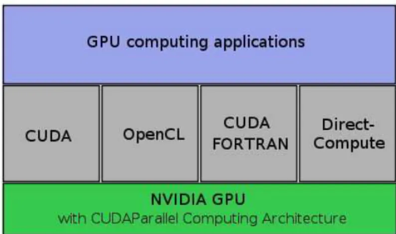
CUDA is an acronym standing for Compute Unified Device Architecture. It is a parallel computing platform and programming model created by NVIDIA and implemented in their graphics processing units (GPUs). CUDA provides the access to the virtual instruction set and memory of the parallel computational elements in CUDA GPUs. Thanks to CUDA, the latest NVIDIA GPUs become accessible for computation like CPUs. GPUs have a parallel throughput architecture that emphasizes executing many concurrent threads slowly rather than executing one single thread very quickly. The arrival of CUDA leverages a powerful parallel compute engine in NVIDIA GPUs to solve many complex computational problems in a more efficient way than on CPUs. Normally, the approach of solving general-purpose (not exclusively graphics) problems on GPUs with CUDA is known as GPGPU.

CUDA gives developers a software environment that allows using C as a high-level pro-gramming language. As illustrated in Fig. 2.5, other languages or application program-ming interface are supported, such as CUDA FORTRAN, OpenCL and DirectCompute. When CUDA is executed on GPUs, all the threads will be grouped into blocks and then into warps. All the threads in one block are executed on one SM together. One SM can also have multiple concurrently running blocks. The number of blocks, which are running on one SM, is determined by the resource requirements of each block, such as the number of registers and shared memory usage. The blocks, which are running on one SM at a given time, are called active blocks in this paper. Since typically one block has several warps and the number of warps is the same as the number of threads in one block divided by 32, the total number of active warps per SM is equal to the number of warps per block times the number of active blocks.

Generally speaking, the scheduling of warps is realized by SMs automatically and se-quentially. We take a block of 128 threads as an example. The threads in this block will

Figure 2.5: CUDA is Designed to Support Various languages or Application Programming Inter-faces.

be grouped into four warps: 0-31 threads may be in Warp 1, 32-63 threads may be in Warp 2, 64-95 threads Warp 3 and 96-127 threads Warp 4. However, if the number of threads in the block is not a multiple of 32, the SM (the warp scheduler) will take all the threads left as the last warp. For example, if the number of threads in the block is 66, then there will be three warps: Warp 1 contains 0-31 threads, Warp 2 contains 32-63 threads and Warp 3 takes 64-65 threads. Since the last warp has only two threads, it leads to the waste of computation capability of 30 threads.

Figure 2.6: Warp execution on SM. The waiting warps will be replaced by the ready warps to hide latency.

At any moment, one SM executes only one warp from one block. But this does not imply that SM will certainly finish all the instructions in this warp all at once. If the executing warp needs to wait for some more information or data (for example: reading from/writing in the global memory), a second warp will be shifted into the SM to replace the executing warp for the purpose of hiding latency, as shown in Fig. 2.6. So there should be one theoretically best situation for performance: all the SMs have enough warps to shift if it is necessary, and all the SMs are busy in the execution duration. It is one of the key points to obtain high performance. And it is the reason why, it is necessary to use the threads and blocks in a way that maximizes hardware utilization. In other words, best performance can be reached when the latency of each warp is completely hidden by other warps [OHL+_{08, JD10]. To achieve this, a GPU application can be tuned by two} leading parameters: the number of threads per block and the total number of threads.

2.3.2/ SPMD PARALLEL PROGRAMMING PARADIGM

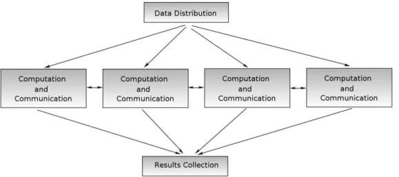
The Single-Program Multiple-Data (SPMD) paradigm is the most used paradigm in par-allel algorithm designing. In this paradigm, processors execute basically the same piece of code but on different parts of the data, which involves the splitting of application data among the available processors. In some other papers, this paradigm is also referred to as geometric parallelism, domain decomposition, or data parallelism. A schematic representation of this paradigm can be seen in Fig. 2.7

Figure 2.7: Basic processing structure of SPMD paradigm.

The applications in this document all have an underlying regular geometric structure, such as the image plane with pixels in stereo matching applications, structured meshing prob-lem, and city distribution in plane in TSP. This allows the data to be distributed among the processors following a given way, where each processor will be in charge of a defined spatial area. Processors communicate with neighboring processors and the communi-cation load will be proportional to the size of the boundary of the input element, while the computation load will be proportional to the volume of the input element. In certain platforms, it may also be required to perform some global synchronization periodically among all the processors. The communication pattern is usually highly structured and extremely predictable. The data may initially be self-generated by each process or may be read from the main memory space during the initialization stage.

SPMD applications can be very efficient if the data are well distributed among the proces-sors and the system is homogeneous. If different procesproces-sors present different workloads or capabilities, then the paradigm should require the support of some load-balancing scheme able to adapt the data distribution layout during run-time execution [SB08]. It should be noted that this paradigm is highly sensitive to the loss of some processors. Usually, the loss of a single processor is enough to cause a deadlock in the computation processing, in which none of the processors can reach the global synchronization point if it exists.

2.3.3/ THREADS IN CUDA

The CUDA programming model follows SPMD software model. The GPU is treated as a coprocessor that executes data-parallel kernel functions. All CUDA threads are organized into a two level concepts: CUDA grid and CUDA block. A kernel has one grid which contains multiple blocks. Every block is formed of multiple threads. The dimension of grid and block can be one-dimension, two-dimension or three-dimension. Each thread has a threadId and a blockId, which are built-in variables defined by the CUDA runtime to help user locate the thread’s position in its block, as well as its block’s position in the grid [NVI12a, SK10].

CUDA provides three key abstractions: one hierarchy of thread groups, device memories and barrier synchronization. Threads have a three-level hierarchy. One block is com-posed of tens of or hundreds of threads. Threads within one block can share data using shared memory and can be synchronized at a barrier. All threads within a block are exe-cuted concurrently on a multi-threaded architecture. A grid is a set of thread blocks that executes a kernel function. Each grid consists of blocks of threads. Then, programmers specify the number of threads per block and the number of blocks per grid.

2.3.4/ SCALABILITY

The advent of GPUs, whose parallelism continues to scale with Moore’s law, bring parallel systems into real applications. The challenge left is to develop computational application software, which transparently scales its parallelism to leverage the increasing number of processor cores, such as 3D graphics applications transparently scale their parallelism to GPUs with widely varying numbers of cores.

Figure 2.8: Scalable programming model.

The CUDA parallel programming model is designed to overcome this challenge, while maintaining a low learning curve for programmers familiar with standard programming

languages, such as C or C++. In fact, the CUDA is simply exposed to the programmers as a minimal set of language extensions of C, even with the three key abstractions of its core: a hierarchy of thread groups, special memory spaces and barrier synchronization. These abstractions provide very fine-gained data and thread parallelism. They guide programmers to partition their problems into coarse sub-problems, that can be solved independently in parallel by blocks of threads, and further each sub-problem into finer pieces that can be solved cooperatively in parallel by all threads within the same block. This decomposition preserves language expressivity, by allowing threads to cooperate when solving each sub-problem, and at the same time, enabling automatic scalability. As it is illustrated in Fig. 2.8, only the runtime system needs to know the count of physical processors. While each block of threads can be scheduled on any of the available pro-cessor cores in any order, a compiled CUDA program can be executed on any number of processor cores.

2.3.5/ SYNCHRONIZATION EFFECTS

The CUDA programming model supports thread synchronization through the sync-threads() function. Typically, all the threads are executed asynchronously whenever all the source operands in a warp are ready. However, if we take this function into count, it will stand as a barrier synchronization function, that makes the threads in the same block coordinate their activities, which will guarantee that all the simultaneously activated threads are in the same location of the program sequence at the same time, thus ensuring that all the threads are reading the correct values from the relative memory space.

Figure 2.9: Additional delay effects of thread synchronization.

When a kernel calls syncthreads() function, threads of the same block will be stopped until all the threads of the block reach the sync-location1. While this may seem to slow down execution since threads will be idle if they reach the sync-location before other threads, it is absolutely necessary to sync the threads here, because the additional delay 1_{It should be noticed that CUDA has no barrier for synchronize the blocks of a grid, thus blocks can} execute in any order relative to each other

is surprisingly less than one waiting period, in almost all the applications [NVI10]. Fig. 2.9 shows the additional delay effect.

2.3.6/ WARP DIVERGENCE

An undesirable effect of having data dependent branching in flow control instruction (if, for, while) is warp divergence. This can slow down the instruction throughput when threads of the same warp follow different execution paths. In that case, the different execution flows in a warp are serialized. Since threads of a same warp share a program counter, this increases the number of instructions executed for this warp. Once all executed paths are completed, the warp converges back to the same execution path. Full efficiency arises when all 32 threads of a warp follow a common path. But these conditions look difficult to obtain in data dependent applications with non-uniform distributions.

2.3.7/ EXECUTION CONFIGURATION OF BLOCKS AND GRIDS

The dimension (both the width and the height) and size (total number of elements) of a grid and the dimension and size of a block are both important factors. The multidimen-sional aspect of these parameters allows easier mapping of multidimenmultidimen-sional problems to CUDA GPU even if it does not play a role in performance. As a result, it is more interesting to take the ‘size’ into discussion rather than the ‘dimensions ’.

The number of active warps per multiprocessor has a great influence on the latency hid-ing and occupancy. This number is implicitly determined by the execution parameters along with resource constraints, such as registers or/and other memory space on chip. The choosing of execution parameters maintains a balance between the latency hiding, occupancy and the resource utilization. There do exist some certain heuristics that can be individually applied to each parameter [NVI11]. When choosing the first execution configuration parameter, the number of blocks per grid, the primary concern is keeping the entire GPU busy. It is better to make the grid size larger than the number of multipro-cessors, so that all multiprocessors have at least one block to execute. Moreover, there should be multiple active blocks per multiprocessor, so that blocks that are not waiting for a synchronization function ( syncthreads()) can keep the hardware busy. This rec-ommendation is subject to resource availability, so, it should be determined along with a second execution parameter, the number of threads per block and the usage of memory-on-chip, such as shared memory.

When choosing the block size, it is important to keep in mind one phenomenon, that multiple concurrent blocks can reside on a multiprocessor and therefore occupancy is not determined only by block size alone. In other words, a larger block size does not necessarily lead to a higher occupancy. For example, on a device of computation capacity 1.1 or lower, a kernel with a maximum block size of 512 threads results in an occupancy of 66 percent, because the maximum number of threads per multiprocessor on such a device is 768. Hence, only a single block can be active per multiprocessor. However, a kernel with 256 threads per block on such a device can result in 100 percent occupancy with three resident active blocks [NVI10].

However, higher occupancy does not always mean better performance. A lower pancy kernel will evidently have more registers available per thread than a higher

occu-pancy kernel, which may result in less register spilling to local memory. Typically once an occupancy of 50 percent has been reached, additional increases in occupancy do not necessarily translate into improved performance [Gup12].

With respect to such factors involved in selecting block size, inevitably trial configurations are required. Given the knowledge of occupancy, there still exist a few rules of thumb to help us set the block size for a better performance:

• Threads per block should be a multiple of warp size to avoid wasting computation on under-populated warps and to facilitate coalescing.

• A minimum of 64 threads per block should be used, but this should happen only if there are multiple concurrent blocks per multiprocessor.

• Between 128 and 256 threads per block can be a better choice than others and a good initial range for experimentation with different block sizes.

• It can be very helpful to use some smaller thread blocks rather than one large thread block per multiprocessor if the performance is too much affected by latency, especially when the kernels frequently call the synchronization function ( sync-threads()).

2.4/

C

In this chapter, we have briefly presented the GPU’s parallel architecture and the CUDA programming environment. We first presented the GPU architecture, lying out the two cases of memory accesses: the coalesced access and the uncoalesced access to mem-ory space, figuring out that it is more suggested to reach the coalesced access for efficient data read/write in the main memory space. Then, we explained the CUDA programming model, with the presentation of the scalable programming model and the introduction of configuration of blocks and grids in multi-thread execution. At last, we have drawn out the basic frame of the parallel programming platform. In next two chapters, we will present the background of the problems and applications addressed in this document.

3

B

ACKGROUND ON STEREO

-

MATCHING

PROBLEMS

3.1/

I

This chapter is centered at the presentation of the background of the stereo-matching problems. We first give a definition of stereo-matching problem, lying out its geometry model and the important definitions used in the document. After that, is the presentation of the stereo-matching method, on which we focus at the local matching methods includ-ing their mostly used matchinclud-ing costs and their update in color stereo-matchinclud-ing problems. The left-right consistency check is mentioned as the common used outlier detector for removing the matching errors in the estimated disparity maps. Then, we provide general introductions to the two applications studied in this document: the CFA stereo-matching problem and the real-time stereo-matching implementation. Finally, we enumerate the current research progress in stereo-matching methods.

3.2/

D

In the field of automotive vehicles or robot system, main recent applications require the perception of the three-dimensional real world. In this case, the intelligent vehicle system, used in assisting the driver and warning him when there is a potential danger, should be able to detect the different objects that are on the road, and represent them in the three-dimensional scene map. Here, we focus on artificial devices such as stereo cameras, equipped with two cameras, to mimic and simulate the mainly used detecting system, that is, the human-eyes bionic stereovision system. Two images of the scene are acquired simultaneously by the cameras. From these two images (left image and right image), stereovision system aims to recover the third dimension, which has been lost during the image formation. The projections of the same scene point visible by the two cameras do not have the same coordinates in the two image planes. The exact position of this scene point can be retrieved if its two projections, called homologous pixels, are identified. The problem of identifying homologous pixels in the two images is called stereo-matching problem.

Stereo matching methods are applied to pairs of stereo images that can be gray-level images or color images. In gray-level images each pixel is characterized by a gray-level intensity value, while in color images each pixel is characterized by three color compo-nents Red (R), Green (G) and Blue (B) intensities.

Figure 3.1: Binocular Stereovision Geometry.

In a classic binocular stereoscopic vision, from a scene point P, using the projection matrices of the left and the right cameras, we can find the location of the projected points onto the left and the right image plans, as illustrated in Fig. 3.1. There is a very interesting set of properties, called epipolar geometry, related to the classic binocular stereovision. Several terms are defined as following:

• the epipolar plane of a scene point P is the plane determined by P and the projec-tion centers Ol and Or.

• the left epipolar is the projection onto the left projection plane of the right projection center and theright epipolar is the projection onto the right projection plane of the left projection center.

• to any space point, we associate two epipolar lines which are in overlap as one line in Fig. 3.1. The epipolar lines are the intersections of the epipolar plane of the point with the projection planes. In the figure, the epipolar line is the projection of the straight line OlPor OrPonto the right or the left projection plane, respectively.

The epipolar geometry describes the relation between right and left projections of a scene point P. Hence, the very important property, called epipolar property is introduced:given a scene point P, its right projected point pr lies on the right epipolar line corre-sponding to its left projected point pl and vice versa.

Now suppose an inverted problem, the two projected points are identified and we want to find the location of scene point P. P is the intersection of the straight lines Olpl and Orpr. So the scene point P can be recovered if only the pair of left and right projected points is identified. Given only one projection of a scene point P, the stereo-matching problem aims at determining its homologous one in the other image plan if it exists.

As we know, for one projection p, its homologous projection p’, if it exists, lies on the epipolar line corresponding to the projection p. However, in the binocular model, the two epipolar lines coincide with each other. So, the correspondence problem is in fact a one-dimensional search problem rather than one two-one-dimensional search problem. However, the homologous point might not even exist in certain cases, such as half-occlusion.

3.2.1/ HALF-OCCLUSION

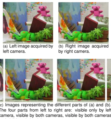
In binocular stereovision, since there are some scene points that can be visible by only one camera, we cannot project every scene point onto two image plans [OA05]. We refer to these points as half-occluded. The Fig. 3.2 presents this very half-occlusion phenomenon and the Fig. 3.3 shows a more concrete example. In Fig. 3.2, the scene B is projected onto bl in the left image plane but is not visible by the right camera. Similarly, the scene point C is projected onto crin the right image plane but is not visible by the left camera. We can deduce that all the scene points between A and B are invisible for the right camera, while the scene points between C and D are invisible for the left camera.

Figure 3.2: Half-occlusion Phenomenon.

(a)Left image acquired by left camera.

(b) Right image acquired

by right camera.

(c)Images representing the different parts of (a) and (b). The four parts from left to right are: visible only by left camera, visible by both cameras, visible by both cameras and visible only by right camera.

3.2.2/ ORDER PHENOMENON

In the stereovision model, an assumption is usually taken: a group of scene points has the same projection rank order in both image plans. Fig. 3.4(a) presents a case that respects this order. However, this hypothesis of order conservation does not always hold true. For example, when the scene points belong to objects at different distances from cameras, this order is not respected any more, as illustrated in Fig. 3.4(b).

(a) Order Respected. (b) Order Not Respected.

Figure 3.4: Order Phenomenon.

3.3/

S

3.3.1/ METHOD CLASSIFICATION

Generally speaking, a high computational complexity is not avoidable for methods to solve the stereo-matching problem by analyzing a pair of stereo images. Particularly, for each pixel in the left image, there are a lot of possible candidate right pixels to be examined in order to determine the best correspondence. It is assumed that the homologous right pixel corresponds to the best correspondence. Stereo-matching methods can be sorted into two classes: the sparse methods and the dense methods [Wor07].

Sparse methods match features that have been identified in the stereo image pair. The features used can be edges, line segments, curve segments and so on. For this reason, these methods are also called feature-based methods. the matching process is carried out only on the detected features [Wu00]. These methods draw significant attention for many years since 1980s because of their low computational complexity. In that time, they are well suited for real-time applications [MPP06]. However, these methods can not satisfy those applications that need an accurate identification of all the homologous pixels in the stereo image pair [BBh03]. This turns people to dense methods in the last decade. The dense matching methods are the stereo-matching methods that provide all the ho-mologous pixels in the stereo image pair. The two methods proposed in this document are both dense matching methods. Since there are a large amount of papers about solv-ing the stereo-matchsolv-ing problem, it is quite difficult to make an exhaustive review. But

as these methods do have the same processing steps, a brief review of recent dense stereo-matching methods has been done by Scharstein and Szeliski [SS02].

3.3.2/ DENSE STEREO-MATCHING METHOD

The four steps which are usually performed by a dense stereo-matching method are identified:

• Matching cost computation.

• Cost aggregation where the initial matching costs are spatially aggregated over a support region of a pixel.

• Optimization to determine the best correspondence at each pixel. • Matching results refinement to remove the outliers.

The dense matching methods are further classified into global methods and local meth-ods. The optimization step of global methods involves a high computational effort which does not make them suitable for real-time applications. Although global methods can pro-vide very good results [SS02, BBh03], the interest in local methods does not decrease thanks to their simplicity and low computational complexity, and the local methods have the top performance [Mei11, SWP+_{12] in the list of Middlebury [HS06].}

In a context of GPU computation, local dense stereo-matching methods, which are also called window-based approaches, are the natural choice for parallel computation. These methods assume that the intensity configurations are similar in the neighborhood of ho-mologous pixels. Particularly, intensity values of neighbors of a pixel in the left image are closed to those of the same neighbors of its homologous pixel in the right image. So, a matching cost is defined between the window around the left pixel and the window around the candidate pixels in the right pixels. The window is also called support region.

3.3.3/ MATCHING COST COMPUTATION

Common pixel-based matching costs include absolute differences (AD), sum of abso-lute differences (SAD), squared differences (SD), sum of squared differences (SSD) and sampling-insensitive absolute differences [BT98], or their truncated versions. A detailed review about matching costs is provided by [HS07]. Since stereo-matching costs are used by window-based stereo methods, they are usually defined for a given window shape. For a fixed window in a level image, the Absolute Difference (AD), between the gray-level Il(xl,y)of pixel plwith coordinates (xl,y)in the left image and the gray-level Ir(xl− s, y) of a candidate pixel pr at a shift s with coordinates (xl− s, y) in the right image, is defined in Equation 3.1, where the subscript g refers to gray-level images. The Sum of Absolute Differences (SAD) is defined as Equation 3.2. The SAD measures the aggregation of absolute differences between the gray-levels of pixels, in support region of size (2w + 1) × (2w + 1) centered at pl and a similar window at pr, with w the window’s half-width.

S ADg(xl,y, s) = w X i=−w w X j=−w |Il(xl+ i, y + j)− Ir(xl+ i− s, y + j)| (3.2) Similarly, the Squared Difference (SD) and the Sum of Squared Differences (SSD) are defined in Equation 3.3 and Equation 3.4, respectively.

S Dg(xl,y, s) = (Il(xl,y)− Ir(xl− s, y))2 (3.3) S S Dg(xl,y, s) = w X i=−w w X j=−w (Il(xl+ i, y + j)− Ir(xl+ i− s, y + j))2 (3.4)

In color images, for each pixel at coordinates (x, y), the presentation of the pixel’s dense information is associated with three color components rather than one component in gray-level images. So, to present a point in three-dimensional RGB color space, the coordi-nates of the color point should be updated as R(x, y), G(x, y) and B(x, y). Therefore, a color image can be considered as an array of color points I(x, y) = (R(x, y), G(x, y), B(x, y))T_{. And} the color image can be split into three component images R, G and B, in each of these images, a point is characterized by one single color component level as in gray-level im-ages. A lot of research has shown that the use of color images rather than gray-level ones can highly improve the accuracy of stereo-matching results [Cha05, CTB06, Kos96]. The color information can be sometimes helpful in reducing stereo-matching ambiguities as presented by [CTB06]. Anyway, in most cases, a full color image carries more information in its three color components than a gray-level image of the same scene.

The generalization to color images of stereo-matching costs should also be updated. Based on Equation 3.1 and Equation 3.2, the matching cost AD and SAD are rewritten as Equation 3.5 and Equation 3.6.

ADc(xl,y, s) =|Rl(xl,y)− Rr(xl− s, y)| + |Gl(xl,y)−Gr(xl− s, y)| + |Bl(xl,y)− Br(xl− s, y)| (3.5)

S ADc(xl,y, s) = w X i=−w w X j=−w (_|Rl(xl+ i, y + j)− Rr(xl+ i− s, y + j)| +|Gl(xl+ i, y + j)− Gr(xl+ i− s, y + j)| +|Bl(xl+ i, y + j)− Br(xl+ i− s, y + j)|) (3.6)

Similarly, the SD and SSD can be generalized to deal with color images as Equation 3.7 and Equation 3.8. Where the k·k is the Euclidean norm, and therefore, k·k2_{is the squared} Euclidean distance between two points of the three-dimensional RGB color space. And Il and Irare the color points associated respectively with the left and right pixels [Kos93].

S Dc(xl,y, s) =kIl(xl,y)− Ir(xl− s, y)k2 (3.7) S S Dc(xl,y, s) = w X i=−w w X j=−w kIl((xl+ i, y + j)− Ir(xl+ i− s, y + j)k2 (3.8)

The matching cost will be computed by shifting the window over all the possible candidate pixels in the right image. The final estimated disparity is determined by the shift where the matching cost reaches the minimum. All the local stereo-matching methods use the window in a certain way and they are also called area-based or window-based matching methods.

3.3.4/ WINDOW FOR COST AGGREGATION

Local dense matching methods exploit the concept of support region or window. Every pixel receives a support from its neighbor pixels. It is commonly accepted that pixels inside this support region are likely to have the same disparity and can therefore help to resolve matching ambiguities. Usually, the support region can be classified into fixed window and adaptive window.

A straightforward aggregation approach consists in using a square window centered at each pixel p. This kind of square-window approach implicitly assumes that the disparity is similar over all pixels in square window. However, this assumption does not hold true near discontinuity areas. To overcome this problem, several works have been done [BI99, FRT97], and the shifting window approach is proposed for this purpose. This approach considers multiple square windows centered at different locations and retains the window with the smallest cost. The size of the support window is fixed and is difficult to adjust the size for both square-window and shifting-window approaches. A small window may not include enough intensity values for a good matching result, while a large one may violate the assumption of constant disparity inside the support window. In fact, the window size should be able to represent the shape of objects in one image. Thus, the window size should be large for textureless regions and small for well textured regions. For this reason, Kanade et al [KO94] proposes an adaptive-window method which automatically selects the window size and/or shape based on local information. We will retain this method for improving our GPU method.

3.3.5/ BEST CORRESPONDENCE DECISION

After the computation and aggregation of matching cost, the homologous pixel in the right image is derived based on the Winner-Takes-All (WTA) principle, as illustrated in Fig. 3.5. The shift for which the matching cost is the lowest is selected. Thus, the estimated disparity ˆd_lw(xl,y)at the pixel pl corresponds to the shift s of the right pixel at which the matching cost is the minimum. It can be expressed as Equation 3.9 when the SAD matching cost is used.

ˆ

dw_l (xl,y) = arg min s (S AD

w

g(xl,y, s)) (3.9)

In this document, the left image pixel is used as the reference in the cost computation as default. So, we use the l subscript in the estimated disparity symbol, s ranging from smin to smax. And the superscript w is taken into use when the aggregation is based on a neighborhood window with a half-width w.

Once the disparity has been estimated at each pixel in the left image, the left dense estimated disparity map is formed. The disparity map is the array of disparity values

✲s ✻

Matching Cost

smin dˆω_l (xl,y) smax

Figure 3.5: Winner-Takes-All method, [smin,smax] represents

the possible shifts of the searched pixels. When the shifts

s equals to ˆd (estimated disparity), the matching cost value reaches the minimum.

computed for each pixel, which has the same size as the input left image and right image. However, the matching cost does not always reach a global extremum at the correct dis-parity for all the regions, Fig. 3.6 illustrates three examples of untextured area, textureless area and repetitive area [Cha05], respectively. In these cases, the gray-levels of the left image and right image are represented. If we examine the gray-level of nine pixels, we are not able to determine a correspondence in the right image, because the gray-level pattern is the same along the correspondence epipolar lines in the two images. As a re-sult, several minimums are found, which will shield the true disparity from being chosen. To avoid this problem, the matching cost and the aggregation support region should be carefully chosen to correctly match pixels.

3.3.6/ LEFT-RIGHT CONSISTENCY CHECK

In the matching process, one image is taken as a reference, for each pixel in this image, we seek its homologous pixel in the other image. The matching method may yield one estimated disparity map for each of the two input images. The first one is for the left input image and the second one is based on the right image. On these two estimated disparity maps, there could be some matching errors. So, a refinement step is usually employed to improve the matching quality.

Different methods allow the refinement to improve the disparity estimation quality. These refinement methods are variously used in most stereo-matching methods [FHZF93]. And they are employed as a post-processing step to improve disparity maps by removing those false matching results or for providing sub-pixel disparity estimation.

The most used method for detecting false matching results is the left-right consistency check. This consistency check method takes the estimated disparity as outlier if Equation

(a)

(b)

(c)

Figure 3.6: Matching cost reaches several minimum. (a) Untextured regions. (b) Textureless regions. (c) Repetitive texture regions.

3.10 does not hold true. ˆ

dw_l (xl,y) = ˆdr(xr,y) = ˆdr(xl− ˆdl(xl,y), y) (3.10) If this condition is not verified, then it is considered that this pixel may be bad matched and should be repaired, or lying in a half-occlusion region, and so, no disparity value can be estimated at this pixel [FRT00].

3.4/

T

-

In this document, two problems of stereo-matching and their related methods are studied and implemented with GPU computing. They are the CFA stereo-matching problem and the real-time stereo-matching. Here, we briefly present their main characteristics.

3.4.1/ INTRODUCTION TOCFA STEREO-MATCHING PROBLEMS

In most real-time implementation of stereo-matching, such as the intelligent cars and the integrated robot systems, the color image pairs can be acquired by two types of cameras: the one equipped with three sensors associated with beam splitters and color filters, providing the so-called full color images, of which each pixel is characterized in Red, Green and Blue levels, and the one equipped only with a single-sensor.

In the second case, the single-sensor cannot provide a full color image directly, but actu-ally deliver a color filter array (CFA) image. Every pixel in it is characterized by a single color component, that can be one of the three color components: Red (R), Green (G) and Blue (B). So, the missing color components have to be estimated at each pixel. This pro-cess of estimating the missing color components is usually referred as CFA demosaicing. It produces a demosaiced color image where every pixel is presented by an estimated color point [BGMT08].

As the demosaicing methods intend to produce demosaiced color images, they attempt to reduce the presence of color artifacts, such as the false colors or zipper effects, by filtering the images [YLD07]. So some useful color information for stereo-matching may be lost in the color demosaiced images. As a result, the demosaiced color image pairs’ stereo-matching quality usually suffers either from color artifacts or from the alteration of color texture caused by demosaicing schemes.

The method that is presented by Halawana [Hal10] is an alternative solution to match pixels by analyzing directly the CFA images, without reconstructing all the full color image by demosaicing processing. These type of stereovision is called CFA stereo-matching problem. We present and study a GPU implementation of the Halawana method in this document.

3.4.2/ INTRODUCTION TO REAL-TIME STEREO-MATCHING METHODS

The constraint of computation time in stereo-matching methods is very important for ap-plications that run at video rate. So, the running time of stereo-matching methods used

should be less than 34 ms, which is generally the image acquisition time in filming the videos. The research work about real-time stereo-matching follows two main ways:

• looking for algorithms with low computation time while still providing good matching quality,

• developing hardware devices for efficient implementation in order to decrease the computation time.

These devices include special purpose hardware, such as the digital signal processors (DSP) or field programmable gate arrays (FPGA), and extensions to recent PCs, for ex-ample, the Multi-media Extension (MMX) [FKO+_{04, HIG02] and the pixel/vertex shading} instructions for the Graphics Processing Units (GPUs) [GY05, MPL05].

3.5/

R

-

3.5.1/ CURRENT PROGRESS IN THE REAL-TIME STEREO COMPUTATION

From the beginning of 1990s, real-time dense disparity map stereo has become a re-ality, making the use of stereo processing feasible for a variety of applications. Until very recently, all near real-time implementations made use of special purpose hardware, like digital signal processors (DSP) or field programmable gate arrays (FPGA). However, with ever increasing clock speeds and the integrating of single instruction multiple data (SIMD) coprocessors, such as Intel MMX, the NOC and the Graphic Processing Unit (GPU) into general-purpose computers, near real-time stereo processing becomes a re-ality for common personal computers. This section presents the progression of fast stereo implementation over the last two decades.

In 1993, Faugeras et al reported on a stereo system developed at INRIA and imple-mented it for both DSP and FPGA hardware [FHZF93]. They impleimple-mented normalized correlation efficiently using the block matching method with left-right consistency check-ing. They used a right-angle trinocular stereo configuration, computing two estimated disparity maps and then merging them to enforce joint epipolar constraints. The DSP implementation exploited the MD96 board [Mat93], that consists in four Motorola 96002 DSPs. The other implementation on FPGA was designed for the PeRle-1 board; which was developed at DEC-PRL and was composed of 23 Xilinx logic cell arrays (LCA). The algorithms were also implemented in C for a Sparc 2 workstation. The results showed that the FPGA implementation outperformed the DSP implementation by a factor of 34 and the Sparc 2 implementation by a factor of 210, processing 256 × 256 pixel images at approximately 3.6 fps.

In the same year, Nishihara presented a stereo system based on the PRISM-3 board developed by Teleos Research [Nis93]. This system used Datacube digitizer hardware, custom convolver hardware, and the PRISM-3 correlator board, which makes extensive use of FPGAs. For robustness and efficiency, this system employed area correlation of the sign bits after applying a Laplacian of Gaussian filter to the images. Two years later, Konolige also reported on the performance of a PC implementation of these algorithms by Nishihara in 1995 [Kon97]. His system was capable of 0.5 fps with 320 × 320 pixel images.