Differential approximation results for the traveling salesman
problem with distances 1 and 2
J´erˆome Monnot Vangelis Th. Paschos∗ Sophie Toulouse {monnot,paschos,toulouse}@lamsade.dauphine.fr
Abstract
We prove that both minimum and maximum traveling salesman problems on complete graphs with edge-distances 1 and 2 (denoted by min TSP12 and max TSP12, respectively) are approximable within 3/4. Based upon this result, we improve the standard approximation ratio known for maximum traveling salesman with distances 1 and 2 from 3/4 to 7/8. Finally, we prove that, for any ² > 0, it is NP-hard to approximate both problems better than within 741/742 + ². The same results hold when dealing with a generalization of min and max TSP12, where instead of 1 and 2, edges are valued by a and b.
1 Introduction
Given a complete graph on n vertices, denoted by Kn, with edge distances either 1 or 2 the mini-mum traveling salesman problem (min TSP12) consists of minimizing the cost of a Hamiltonian cycle, the cost of such a cycle being the sum of the distances on its edges (in other words, in finding a Hamiltonian cycle containing a maximum number of 1-edges). The maximum traveling salesman problem (max TSP) consists of maximizing the cost of a Hamiltonian cycle (in other words, of finding a Hamiltonian cycle containing a maximum number of 2-edges). A generaliza-tion of TSP12, denoted by TSPab, is the one where the edge-distances are either a, or b, a < b. Both min and max TSP12, and TSPab are NP-hard.
Given an instance I of an NP optimization (NPO) problem Π and a polynomial time approx-imation algorithm A feasibly solving Π, we will denote by ω(I), λA(I) and β(I) the values of the worst solution of I, of the approximated one (provided by A when running on I), and the optimal one for I, respectively. Generally (see [8]), the quality of an approximation algorithm for an NP-hard minimization (resp., maximization) problem Π is expressed by the ratio (called standard in what follows) ρA(I) = λ(I)/β(I), and the quantity ρA = inf{r : ρA(I) < r, I instance of Π} (resp., ρA = sup{r : ρA(I) > r, I instance of Π}) constitutes the approximation ratio of A for Π. Another approximation-quality criterion used by many researchers ([2, 1, 3, 4, 13, 14]) is what in [6, 5] we call differential-approximation ratio. It measures how the value of an approxi-mate solution is placed in the interval between ω(I) and β(I). More formally, the differential-approximation ratio of an algorithm A is defined as δA(I) = |ω(I) − λ(I)|/|ω(I) − β(I)|. The quantity δA = sup{r : δA(I) > r, I instance of Π} is the differential approximation ratio of A for Π. In [2], the term “trivial solution” is used to denote the solution realizing the worst among the feasible solution-values of an instance. Moreover, all the examples in [2] carry over NP-hard problems for which worst solution can be trivially computed. This is for example the case of maximum independent set where, given a graph, the worst solution is the empty set, or of min-imum vertex cover, where the worst solution is the vertex-set of the input-graph, or even of the
∗LAMSADE, Universit´e Paris-Dauphine, Place du Mar´echal De Lattre de Tassigny, 75775 Paris Cedex 16,
minimum graph-coloring where one can trivially color the vertices of the input-graph using a distinct color per vertex. On the contrary, for TSP things are very different. Let us take for ex-ample min TSP. Here, given a graph Kn, the worst solution for Knis a maximum total-distance Hamiltonian cycle, i.e., the optimal solution of max TSP in Kn. The computation of such a solution is very far from being trivial since max TSP is NP-hard. Obviously, the same holds when one considers max TSP and tries to compute a worst solution for its instance, as well as for optimum satisfiability, for minimum maximal independent set and for many other well-known NP-hard problems. In order to remove ambiguities about the concept of the worst-value solu-tion of an instance I of an NPO problem Π, we will define it as the optimal solusolu-tion opt(Π0) of an NPO problem Π0 having the same set of instances and feasibility constraints as Π verifying
opt(Π0) = ½
max opt(Π) = min min opt(Π) = max
In general, no apparent links exist between standard and differential approximations in the case of minimization problems, in the sense that there is no evident transfer of a positive, or negative, result from one framework to the other. Hence, a “good” differential-approximation result implies nothing for the behavior of the approximation algorithm studied when dealing with the standard framework and vice versa. When dealing with maximization problems, we show in [10] that the approximation of a maximization NPO problem Π within differential-ap-proximation ratio δ implies its apdifferential-ap-proximation within standard-apdifferential-ap-proximation ratio δ.
The best known standard-approximation ratio known for min TSP12 is 7/6 ([11]), while the best known standard inapproximability bound is 743/742 − ², for any ² > 0 ([7]). On the other hand, the best known standard-ratio max TSP is 3/4 ([12]). To our knowledge, no better result is known in standard approximation for max TSP12. Furthermore, no special study of TSPab has been performed until now (a trivial standard-approximation ratio of b/a or a/b is in any case very easily deduced for min or max TSPab).
Here we show that min and max TSP12, and min and max TSPab are all equi-approximable within 3/4 for the differential approximation. We also prove that all these problems cannot be approximated better than within 741/742 + ², for any ² > 0. By the equi-approximability of min TSP12, max TSP12, min TSPab and max TSPab, the results obtained for the case of min TSP12 apply to the rest of the problems above. Finally, we improve the standard -approximation ratio of max TSP12 from 3/4 ([12]) to 7/8.
In what follows, we will denote by V = {v1, . . . , vn} the vertex-set of Kn, by E its edge-set, and for vivj ∈ E, we denote by d(vi, vj) the distance of the edge vivj ∈ E; we consider that the distance-vector is symmetric and integer. Given a feasible TSP-solution T (Kn) of Kn(both min and max TSP have the same set of feasible solutions), we denote by d(T (Kn)) its (objective) value. Given a graph G, we denote by V (G) its vertex-set. Finally, given any set C of edges, we denote by d(C) the total distance of C, i.e., the quantityP
vivj∈Cd(vi, vj).
2 Differential-approximation preserving reductions for TSP12
In this section we give a differential-approximation preserving result that will be used later. Theorem 1. min TSP12, max TSP12, min TSPab and max TSPab are all equi-approximable for the differential approximation.
Proof. In order to prove the theorem we will prove the following stronger lemma.
Lemma 1. Consider any instance I = (Kn, ~d) (where ~d denotes the edge-distance vector of Kn). Then, any legal transformation ~d 7→ γ.~d + η.~1 of ~d (γ, η ∈ Q) produces differentially equi-approximable TSP-problems.
Proof of lemma 1. Suppose that TSP can be approximately solved within differential-approximation ratio δ and remark that both the initial and the transformed instance have the same set of feasible solutions. By the transformation considered, the value d(T (Kn)) of any fea-sible tour T (Kn) is affinely transformed into γd(T (Kn)) + ηn. Since differential-approximation ratio is stable under affine transformation, the equi-approximability of the original and of the transformed problem is immediately deduced, concluding so the proof of lemma 1.
We are ready now to continue the proof of theorem 1. In order to prove that min TSP12 and max TSP12 are equi-approximable, it suffices to apply lemma 1 proved just above with γ = −1 and η = 3. On the other hand, in order to prove that min or max TSP12 reduces to min or max TSPab, we apply lemma 1 with γ = 1/(b − a) and η = (b − 2a)/(b − a), while for the converse reduction we apply lemma 1 with γ = b − a and η = 2a − b. Since the reductions presented are transitive and composable, the equi-approximability of the pairs (min TSP12, max TSP12) and (TSP12, TSPab) proves the theorem.
For reasons of simplicity, we deal, in what follows, with min TSP12. The differential-approximation results obtained can be immediately transferred, by theorem 1, to max TSP12, min TSPab and max TSPab.
3 Approximating min TSP12
Let us first recall that, given a graph G, a 2-matching is a set M of edges of G such that if V (M ) is the set of the endpoints of M , the vertices of the graph (V (M ), M ) have degree at most 2; in other words, the graph (V (M ), M ) is a collection of cycles and simple paths. A 2-matching is optimal if it is the largest over all the 2-matchings of G. It is called perfect if any vertex of the graph (V (M ), M ) has degree equal to 2, i.e., if it constitutes a partition of V (M ) into cycles in G. Remark that determining a maximum 2-matching in a graph G is equivalent to determining a minimum total-distance vertex-partition into cycles into G ∪ ¯G (the complement of G), where the edges of G are considered of distance 1 and the ones of ¯G of distance 2.
As shown in [9], an optimal triangle-free 2-matching can be computed in polynomial time. As mentioned above, this amounts to computing a triangle-free minimum-distance collection of cycles in a complete graph Kn with edge-distances 1 and 2. Let us denote by M such a collection. Starting from M , we will progressively patch its cycles in order to finally obtain a unique Hamiltonian cycle in Kn.
3.1 Preprocessing M
We first define two operations, namely the 2-exchange and the 2-patching, implying two vertex-disjoint cycles of a 2-matching.
Definition 1. Let C1 and C2 be two vertex-disjoint cycles. Then:
a 2-exchange is any replacement of two edges v1u1 ∈ C1, v2u2 ∈ C2 by the edges v1v2 and u1u2;
a 2-patching of C1 and C2 is any cycle C resulting from a 2-exchange on C1 and C2, i.e., C = (C1∪ C2\ {v1u1, v2u2}) ∪ {v1v2, u1u2}, for any pair (v1u1, v2u2) ∈ C1× C2.
A 2-matching minimal with respect to the 2-exchange operation will be called 2-minimal. In particular, if all edges have the same cost, then a 2-minimal matching is a tour.
Definition 2 . A 2-matching M = (C1, C2, . . . , C|M |) is 2-minimal if it verifies, ∀(Ci, Cj) ∈ M × M , Ci 6= Cj, ∀v1u1∈ Ci, ∀v2u2 ∈ Cj, d(v1, v2) + d(u1, u2) > d(u1v1) + d(u2v2).
In other words, a matching M is minimal if any patching of its cycles produces a 2-matching of total distance strictly greater than the one of M . Starting from a 2-2-matching ˆM transformation of ˆM into a 2-minimal one M can be performed in polynomial time by the following procedure.
BEGIN *2 MIN* Mp ← ∅; REPEAT
pick a new set {Ci, Cj} ⊆ ^M; FOR all vkvl ∈ Ci, vpvq∈ Cj DO
take edges vkvl ∈ Ci and vpvq ∈ Cj; C1 ij← Ci∪ Cj\ {vkvl, vpvq} ∪ {vkvp, vlvq}; C2 ij← Ci∪ Cj\ {vkvl, vpvq} ∪ {vkvq, vlvp}; Cij← argmin{d(C1ij), d(C2ij)}; Mp ← ^M\ {Ci, Cj} ∪ Cij; IF d(^M) > d(Mp) THEN ^M← Mp FI OD
UNTIL no improvement of d(^M) is possible; OUTPUT M← ^M;
END. *2 MIN*
Moreover, suppose that there exist two distinct cycles C and C0 of M (the output of the proce-dure 2 MIN), both containing 2-edges and denote by uv ∈ C and u0v0 ∈ C0 two such edges. Then, d(uu0) + d(vv0) > 4, while d(uv) + d(u0v0) = 4, a contradiction. So, the following proposition holds.
Proposition 1. In any 2-minimal 2-matching, at most one of its cycles contains 2-edges. Remark 1. If the size of a 2-minimal triangle-free 2-matching M is 1, then, since a Hamiltonian tour is a special case of triangle-free 2-matching, M is an optimal min TSP12-solution. Hence, in what follows we will suppose 2-matchings of size at least 2.
Assume now a 2-minimal triangle-free 2-matching M = (C1, . . . , Cp, C0), verifying remark 1, where C0is the unique cycle of M (if any) containing 2-edges. Construct a graph H = (VH, EH); VH = {w1, . . . , wp} contains a vertex per cycle of M and, for i 6= j, wiwj ∈ EH iff ∃(u, v) ∈ Ci×Cj such that d(u, v) = 1. Consider a maximum matching MH, |MH| = q, of H. With any edge wiswjs of MH we associate the pair (Cis, Cjs) of the corresponding cycles of M . So, M can
be described (up to renaming its cycles) as M = q [ s=1 {C1s, C2s} r=p−2q [ t=1 {Ct}[ {C0} (1)
where for s = 1, . . . , q, ∃es∈ V (Cs
1) × V (C2s) such that d(es) = 1.
Consider M as expressed in (1), denote by Vs the set of the four vertices of C1s and C2s adjacent to the endpoints of es, and construct the bipartite graph B = (V1
B∪ V 2
B, EB) where V1
B= {w1, . . . , wr} (i.e., we associate a vertex with a cycle Ct, t = 1, . . . , r), V 2 B = {w
1, . . . , wq} (i.e., we associate a vertex with a pair (C1s, C2s), s = 1, . . . q) and, ∀(t, s), wtws∈ EB iff ∃u ∈ Ct, ∃v ∈ Vs such that d(u, v) = 1. Compute a maximum matching MB, |MB| = q0 in B. With any edge wtws∈ MB we associate the triple (C1s, C2s, Ct). So, M can be described (up to renaming its cycles) as M = q0 [ s=1 {C1s, C2s, C3s} q [ s=q0+1 {C1s, C2s} r0=r−q0 [ t=1 {Ct}[ {C0} (2)
where for s = 1, . . . , q0, ∃fs ∈ V
s× V (C3s) such that d(fs) = 1. In what follows we will reason with respect to M as it has been expressed in (2).
3.2 Computation and evaluation of the approximate solution and a lower bound for the optimal tour
In the sequel, call s.d.e.p. a set of vertex-disjoint elementary paths, denote by PREPROCESS the procedure that starting from a 2-minimal triangle-free 2-matching M leads to (2) and consider the following algorithm.
BEGIN (*TSP12*)
compute a maximum 2-matching ^M in Kn; M← 2 MIN(^M);
M← PREPROCESS(M); D← ∅;
(1) FOR s← 1 TO q0 DO let gs
1 be the edge of Cs1 adjacent to both es and fs; choose in Cs 2 an edge gs2 adjacent to es; choose in Cs 3 an edge gs3 adjacent to fs; D← (D ∪ Cs 1∪ Cs2∪ Cs3\ {gs1, gs2, gs3}) ∪ {es, fs}; OD (2) FOR s← q0+ 1 TO q DO choose in Cs 1 an edge gs1 adjacent to es; choose in Cs 2 an edge gs2 adjacent to es; D← (D ∪ Cs 1∪ Cs2\ {gs1, gs2}) ∪ {es}; OD (3) FOR t← 1 TO r0 DO
choose any edge gt in Ct; D← (D ∪ Ct) \ {gt};
OD
(4) IF there exists in C0 an 1-edge
THEN choose a 2-edge g0 of C0 adjacent to an 1-edge e; ELSE choose any edge g0 of C0;
D← (D ∪ C0) \ {g0}; FI
(5) complete D in order to obtain a Hamiltonian tour T(Kn); OUTPUT T(Kn);
END (*TSP12*)
Clearly, both achievement of a 2-minimal triangle free 2-matching and PREPROCESS can be performed in polynomial time. Moreover, steps (1) to (4) are also executed in polynomial time. Finally, step (5) can be performed by arbitrarily ordering (mod|D|) the chains of the s.d.e.p. D and then, for i = 1, . . . , |D|, adding in D the edge linking the “last” vertex of chain i to the “first” vertex of chain i + 1. Consequently, the whole algorithm TSP12 is polynomial. Finally, remark that C0 may contain either only 2-edges, or both 1- and 2-edges. In the latter case, edge g0 (in step 4) can be any 2-edge in C0, adjacent to an 1-edge of C0.
Lemma 2. d(T (Kn)) 6 d(M ) + q + r0.
Proof. During steps (1) to (4) of algorithm TSP12, set D remains a s.d.e.p. At the end of step (4), D contains M minus the 3q0 + 2(q − q0) + r0 = q0 + 2q + r0 1-edges of the set
∪qs=10 {gs
1, g2s, g3s}∪ q
s=q0+1{gs1, gs2}∪r
0
s=1{gt} minus (if C06= ∅) one 2-edge of C0plus the 2q0+(q−q0) = q0+ q 1-edges of the set ∪qs=10 {es
1, f2s} ∪ q
s=q0+1{e
s}. So D is a s.d.e.p. of size n − (q + r0) − 1 C06=∅
and of total distance d(M ) − (q + r0) − 2.1C06=∅. Completion of D in order to obtain a tour in Kn,
can be done by adding q + r0+ 1C06=∅ new edges. Each of these new edges can be, at worst, of
distance 2. We so have d(T (Kn)) 6 d(M ) − (q + r0+ 2.1C06=∅) + 2(q + r
0+ 1
C06=∅) = d(M ) + q + r
0, q.e.d.
On the other hand, the optimal tour being a special triangle-free 2-matching, the following lemma holds immediately.
Lemma 3. β(Kn) > d(M ).
3.3 Evaluation of the worst-value solution
In what follows in this section we will exhibit a s.d.e.p., with all edges of distance 2 (called 2-s.d.e.p.). Given such a s.d.e.p. W , one can proceed as in step (5) of algorithm TSP12 (section 3.2), in order to construct a Hamiltonian tour Tw whose total distance is a lower bound for ω(Kn).
Denote by E2 the set of 2-edges of cycle C0. If q = 0, i.e., MH = ∅, and if C0 = E2, then the tour computed by TSP12 is optimal.
Lemma 4. If q = 0 and C0 = E2, then δTSP12(Kn) = 1.
Proof. Let k = |V (C0)| = d(M ) − n and set V (C0) = {a1, . . . , ak}. By the fact that M is 2-minimal, all the edges of Kn incident to these vertices have distance 2. On the other hand, between two distinct cycles in the set {C1, . . . , Cp=r0} of M , there exist only edges of distance 2.
Consider the family F = {{a1}, . . . , {ak}, V (C1), . . . V (Cp)}. By the above remarks, any edge linking vertices of two distinct sets of F is a 2-edge. Any feasible tour of Kn (a posteriori an optimal one) integrates the k + p sets of F by using at least k + p 2-edges pairwise linking these sets. Hence, any tour uses at least k + p 2-edges, so does tour T (Kn) computed by algorithm TSP12, q.e.d.
So, we suppose in the sequel that q = 0 ⇒ C0 6= E2. We will now prove the existence of a 2-s.d.e.p. W of size d(M ) + 4(q + r0) − n, where M is as expressed by (2). In the sequel, a path with alternating vertices will denote a path such that no two consecutive vertices lie in the same cycle.
Proposition 2. Between two cycles Ca and Cb of M of size at least k, there always exists a path with alternating vertices from Ca and Cb, which contains at least k 2-edges.
Proof. Let {a1, . . . , ak+1} and {b1, . . . , bk+1} be k+1 successive vertices of two distinct cycles Ca and Cb of size at least k (possibly a1 = ak+1 if |V (Ca)| = k and b1 = bk+1 if |V (Cb)| = k). We will show that there exists a path with alternating vertices from Ca and Cb of size 2k − 1 and of distance at least 3k − 1. Consider paths C = ∪k
i=1{aibi} ∪k−1i=1 {ai+1bi} and D = ∪k+1i=2{aibi} ∪k−1i=1 {aibi+1}. By the 2-minimality of M we get:
∀i = 1, . . . , k max {d (ai, bi) , d (ai+1, bi+1)} = 2 ⇒ d (ai, bi) + d (ai+1, bi+1) > 3 ∀i = 1, . . . , k − 1 max {d (ai, bi+1) , d (ai+1, bi)} = 2 ⇒ d (ai, bi+1) + d (ai+1, bi) > 3 Summing the terms of the expression above member-by-member, one obtains:
k X i=1 (d (ai, bi) + d (ai+1, bi+1)) + k−1 X i=1 (d (ai+1, bi) + d (ai, bi+1)) > 6k − 3 ⇐⇒ d(C) + d(D) > 6k − 3 ⇒ max {d(C), d(D)} >» 6k − 3 2 ¼ = 3k − 1 Application of proposition 2 to any pair (Cs
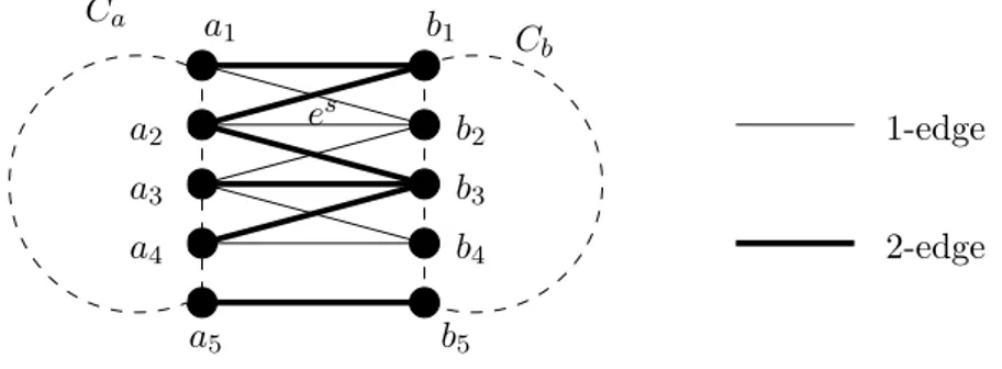
Claim 1. ∀s = 1, . . . , q, there exists a 2-s.d.e.p. Ws of size 4, alternating vertices of cycles Cs 1 and Cs
2, containing a vertex of Vs whose degree with respect to Ws is 1. a1 a2 a3 a4 a5 b1 b2 b3 b4 b5 es Ca Cb 1-edge 2-edge
Figure 1: An example of claim 1. In figure 1, we show an application of claim 1. We assume es = a
2b2; then {a1, b1} ⊂ Vs. The 2-s.d.e.p. Ws claimed is {b
1a2, (a3b3, b3a4), a5b5} and the degree of b1 with respect to Ws is 1. Consider now the s.d.e.p. Ws
t = Ws∪ W0st, where Ws as in claim 1 and W0st is any path of size 4 with alternating vertices from Cs
3 and Ct, s = 1, . . . , q0, t = 1, . . . , r0. By the optimality of MH, any edge linking vertices of C3s to vertices of Ct is a 2-edge. Consequently, Wts is a 2-s.d.e.p. and the following claim holds.
Claim 2. ∀s = 1, . . . , q0, ∀t = 1, . . . , r0, there exists a 2-s.d.e.p. Ws
t of size 8, alternating vertices of the cycles Cs
1 and C2s, and of the cycles C3s and Ct.
For s = q0 + 1, . . . , q, t = 1, . . . r0, consider the triplet (Cs
1, C2s, Ct). Let es = es1es2, Vs = {us
1, vs1, us2, v2s} and consider any four vertices at, bt, ct and dt of Ct. By the optimality of MB, any vertex of Ctis linked to any vertex of Vsexclusively by 2-edges. Moreover, the 2-minimality of M implies that at least one of us
1es2 and es1us2 is of distance 2. If we suppose d(us1, es2) = 2 (figure 2), then the path {es
2, us1, at, v1s, bt, us2, ct, vs2, dt} is a 2-s.e.d.p. Hence, the following claim holds.
Claim 3. ∀s = q0+ 1, . . . , q, ∀t = 1, . . . , r0, there exists a 2-s.d.e.p. Ws
t of size 8, alternating vertices of the cycles Cs
1, C2s and Ct. 2−s.d.e.p. Ct us 1 us2 es 1 es es 2 vs 1 vs 2 at bt ct dt Cs 1 C2s
Figure 2: The 2-s.d.e.p. Ws
Let r0 > 2 and consider, for t = 1, . . . , r0, the (residual) cycles Ct. All edges between these cycles are of distance 2. If we denote by at, bt, ct and dt four vertices of Ct, the path {a1, . . . , at, . . . , ar0, b1, . . . , bt, . . . , br0, c1, . . . , ct, . . . , cr0, d1, . . . , dt, . . . , dr0} is a 2-s.d.e.p. of size
4r0− 1 and the following claim holds.
Claim 4. If r0 > 2, then there exists a 2-s.d.e.p. Wr0
of size 4r0 − 1 alternating vertices of cycles Ct, t = 1, . . . , r0.
Lemma 5. If q > 1, or if [(C0 6= E2) and (r 6= 1)], then δTSP12(Kn) > 3/4.
Proof. Consider M as expressed in (2). Let us denote by W0 a 2-s.e.d.p. on V \ V (C0). From claims 1, 2, 3 and 4: W0= r0 S s=1 Ws s q S s=r0+1 Ws |W0| = 8r0+ 4 (q − r0) = 4 (q + r0) q > r0 q S s=1 WsS Wr0 S {γ} |W0| = 4q + 4r0− 1 + 1 = 4 (q + r0) r0 > q > 0 Wr0 |W0| = 4r0− 1 = 4 (q + r0) − 1 r0 >2, q = 0 (3)
In (3), γ draws an edge linking a vertex of degree 1 with respect to Wr0
to a vertex of degree 1 in V (W0). This last vertex can belong either to V (C1
3) if q0 > 1, or to Vq otherwise. By the optimality of MH and MB, γ is a 2-edge. For the first line of (3), remark that if q = r0, then W0 is given by ∪r0
s=1Wss, and claims 2 and 3 conclude W0 = 8r0 = 4(r0 + q); otherwise (q > r0), claims 1, 2 and 3 conclude the first line of (3). For the second line (r0 > q > 0), since r0 and q are integers, we have r0 > 2. Then, by claim 4, |Wr0
| > 4r0 − 1 and the expression of the second line follows from the fact that γ is a 2-edge. For the third line of (3), claim 4 gives immediately the result. Hence, in any case, W0 is a 2-s.d.e.p. verifying |W0| = 4(q + r0) − 1 if q = 0, |W0| = 4(q + r0) otherwise.
We now construct a a 2-s.e.d.p. W0 on V (C0). Let g0 = u0v0 be the edge removed from C0 during the execution of step (4) of algorithm TSP12. If C0 6= E2, then g0 has been chosen in such a way that one of its endpoints, say v0, is adjacent in C0 to an 1-edge. Let γ0 be an edge linking v0 to a vertex of degree 1 with respect to W0 (such a vertex exists since W0 is acyclic). By the 2-minimality of M , d(γ0) = 2. Set
W0 = ½
E2 \ {g0} ∪ {γ0} |W0| = d(M ) − n C0= E2 E2 ∪ {γ0} |W0| = d(M ) − n + 1 otherwise
Setting finally W = W0∪ W0, one obtains the 2-s.d.e.p. claimed at the beginning of section 3.3. We have d(W ) = 4(q + r0) − 1q=0+ d(M ) − n + 1C06=E2>d(M ) − n + 4(q + r
0), the last inequality holding because of the hypothesis q = 0 ⇒ C06= E2 made just before lemma 2. Any completion of W in a Hamiltonian cycle of Kn(as in step (5) of algorithm TSP12) would produce a tour Tw of total distance d(Tw) > d(M ) + 4(q + r0). So, ω(Kn) > d(M ) + 4(q + r0), and combining this expression together with lemmata 2 and 3, the differential ratio 3/4 is immediately concluded. Lemma 6. If q = 0 and r = 1 and C06= E2, then δTSP12(Kn) > 3/4.
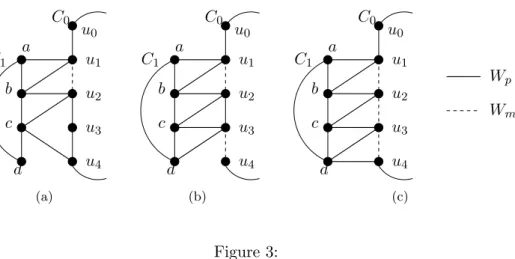
Proof. Recall that, by the optimality of MH, if q = 0 and r = 1, all edges linking cycles C0 and C1 are of distance 2. Let u0, u1 and u2 be three vertices of C0 such that d(u0, u1) = 1 and d(u1, u2) = 2. We denote by u2 a neighbor of u1 with respect to C0, and by u3 6= u1 the neighbor of u2 in C0. Let a, b, c and d be any four vertices of C1, and let Wp and Wm be the sets {au1, u1b, bu2, u2c} and {u1u2}, respectively.
C1 C0 a b c d u0 u1 u2 u3 u4 (a) C1 C0 a b c d u0 u1 u2 u3 u4 (b) C1 C0 a b c d u0 u1 u2 u3 u4 Wp Wm (c) Figure 3:
If u3is adjacent to two 1-edges in C0, i.e., d(u2, u3) = d(u3, u4) = 1, then set Wp= Wp∪{cu4} (figure 3(a)).
If only one of u2u3 and u3u4 is of distance 2, then set Wp = Wp∪ {cu3, u3d} and Wm = Wm ∪ {argmax{d(u2, u3), d(u3, u4)}}. In figure 3(b), sets Wp and Wm are shown for the case where argmax{d(u2, u3), d(u3, u4)} = u3u4, i.e., d(u3, u4) = 2 and d(u2, u3) = 1.
Finally, if u2u3 and u3u4 are both of distance 2 (d(u2, u3) = d(u3, u4) = 2), then set Wp = Wp∪ {cu3, u3d, du4} and Wm= Wm∪ {u2u3, u3u4} (figure 3(c)).
In any of the above cases, we consider the 2-s.d.e.p. W = E2 ∪ Wp \ Wm with |W | = d(M ) − n + 4 = d(M ) − n + 4r0. We then have ω(Kn) > d(M ) + 4r0, and combining it with lemmata 2 and 3, the differential ratio 3/4 is concluded.
In all, combining lemmata 2, 3, 4 and 6, the following theorem can be immediately proved. Theorem 2. min TSP12 is approximable within differential-approximation ratio 3/4.
Theorems 1 and 2 induce the following corollary.
Corollary 1. min TSP12, max TSP12, min TSPab and max TSPab are approximable within differential-approximation ratio 3/4. 1 2 3 4 5 6 7 8 9 10 T∗ Tw T∗ and Tw
Figure 4: Tightness of the TSP12 approximation ratio.
Proposition 3. Ratio 3/4 is tight for TSP12
Proof. Consider two cliques and number their vertices by {1, . . . , 4} and by {5, 6, . . . , n + 8}, respectively. Edges of both cliques have all distance 1. Cross-edges ij, i = 1, 3, j = 5, . . . , n + 8,
k TSP12 The algorithm of [11] 3 0.931100364 0.846702091 4 0.9000002 0.833333 5 0.920289696 0.833333 6 0.9222222 0.833333 D iffer en ti al ra ti o 3 0.923350955 0.87013 4 0.9094018 0.857143 5 0.92646313 0.857143 6 0.928178 0.857143 St anda rd ra ti o
Table 1: A limited comparison between TSP12 and the algorithm of [11] on some worst-case instances of the latter.
are all of distance 2, while every other cross-edge is of distance 1. Unraveling of TSP12 will produce: T = {1, 2, 3, 4, 5, 6, . . . , n + 7, n + 8, 1} (cycle-patching on edges (1, 4) and (5, n + 8)), while Tw= {1, 5, 2, 6, 3, 7, 4, 8, 9 . . . , n+7, n+8, 1} (using 2-edges (1, 5), (6, 3), (3, 7) and (n+8, 1)) and T∗ = {1, 2, n + 8, n + 7, . . . , 5, 4, 3, 1} (using 1-edges (4, 5) and (2, n + 8)). Consequently, δTSP12(Kn+8) = 3/4, q.e.d.
In figure 4, the tours T∗ and Tw of proposition 3 are shown for n = 2. We assume T = {1, . . . , 10, 1}.
Let us note that the differential approximation ratio of the 7/6-algorithm of [11], when running on Kn+8, is also 3/4. The authors of [11] exhibit a family of worst-case instances for their algorithm: one has k cycles of length 4 arranged around a cycle of length 2k. We have performed a limited comparative study between their algorithm and ours, for k = 3, 4, 5, 6 (on 24 graphs). The average differential and standard approximation ratios for the two algorithms are presented in table 1.
Proposition 4 . min TSPab is approximable within standard-approximation ratio ρ 6 (1 + ((b − a)/(4a)). This ratio tends to ∞ when a = o(b).
Proof. Revisit corollary 1. Differential ratio 3/4 for min TSPab implies λ(Kn)/β(Kn) 6 (3/4) + (ω(Kn)/(4β(Kn))). Using ω(Kn) 6 bn and β(Kn) > an, some easy algebra gives the result claimed.
Theorem 3. min and max TSPab and min and max TSP12 are inapproximable within diffe-rential-ratio of at least 742/743 + ², ∀² > 0, unless P=NP.
Proof. Consider min TSP12. Using n 6 β(Kn) 6 ω(Kn) 6 2n, one can see that approximation of min TSP12 within δ = 1−² implies its approximation within ρ = 2−(1−²) = 1+², 0 6 ² 6 1. Then, the inapproximability bound (743/742 − ²) of [7] for min TSP12 together with theorem 1 conclude the proof.
4 An improvement of the standard ratio for the maximum traveling salesman with distances 1 and 2
We propose in this section a non-trivial improvement of the standard-approximation ratio for max TSP12, by proving the following theorem.
Theorem 4 . max TSP12 is polynomially approximable within standard-approximation ratio bounded below by 7/8.
Proof. Combining, as in the proof of proposition 4, expressions δmax TSP12>3/4, ωmax(Kn) > an and βmax(Kn) 6 bn, one deduces ρmax TSP12>(3/4) + (a/4b). Setting a = 1 and b = 2, the result claimed follows immediately.
Remark 2. Consider now the following simple way to use the algorithm of [11] in order to solve max TSP12 on a graph Kn with edge-distances 1 and 2. The graph ¯Kn in the first line of the algorithm MTSPALG just above is such that the distance of an edge e of ¯Kn is 1 if e has distance 2 in Kn, and 2 if e has distance 1 in Kn.
BEGIN *MTSPALG* construct ¯Kn;
call the algorithm of [11] to compute a tour Tmin(¯Kn); OUTPUT Tmax(Kn) ← Tmin(¯Kn);
END.
Let us denote by A the 7/6-algorithm of [11] called in the second line of MTSPALG. Then, by theorem 1, β(Kn) = 3n − β( ¯Kn) and λMTSPALG(Kn) = 3n − λA( ¯Kn), where β(Kn) is the optimal value for max TSP12 on Kn and β( ¯Kn) is the optimal value for min TSP12 on ¯Kn. Then, λA( ¯Kn)/β( ¯Kn) 6 7/6, together with β( ¯Kn) > n imply λMTSPALG(Kn)/β(Kn) > 2/3.
Note finally that standard-approximation ratio 7/8 can be obtained by the following direct method.
BEGIN *max TSP12*
find a triangle-free 2-matching M= {C1, C2, . . .};
FOR all Ci DO delete a minimum-distance edge from Ci OD
properly link the remaining paths to obtain a Hamiltonian cycle T; OUTPUT T;
END. *max TSP12*
Let p be the number of cycles of M where 2-edges have been removed during the FOR-loop of algorithm max TSP12. Then, λmax TSP12(Kn) > d(M ) − p, β(Kn) 6 d(M ), and since M is triangle-free, d(M ) > 8p. Consequently, λmax TSP12(Kn)/βmax(Kn) > 7/8.
The above result, can be extended to the case of max TSPab if we consider that here λmax TSP12(Kn) > d(M ) − p(b − a), β(Kn) 6 d(M ) and d(M ) > 4bp. Hence the following corollary holds and concludes the paper.
Corollary 2. max TSPab is polynomially approximable within standard-approximation ratio bounded below by (3/4) + (a/(4b)).
References
[1] A. Aiello, E. Burattini, M. Furnari, A. Massarotti, and F. Ventriglia. Computational com-plexity: the problem of approximation. In C. M. S. J. Bolyai, editor, Algebra, combinatorics, and logic in computer science, volume I, pages 51–62, New York, 1986. North-Holland. [2] G. Ausiello, A. D’Atri, and M. Protasi. Structure preserving reductions among convex
[3] G. Ausiello, A. Marchetti-Spaccamela, and M. Protasi. Towards a unified approach for the classification of NP-complete optimization problems. Theoret. Comput. Sci., 12:83–96, 1980.
[4] M. Bellare and P. Rogaway. The complexity of approximating a nonlinear program. Math. Programming, 69:429–441, 1995.
[5] M. Demange, P. Grisoni, and V. T. Paschos. Differential approximation algorithms for some combinatorial optimization problems. Theoret. Comput. Sci., 209:107–122, 1998. [6] M. Demange and V. T. Paschos. On an approximation measure founded on the links between
optimization and polynomial approximation theory. Theoret. Comput. Sci., 158:117–141, 1996.
[7] L. Engebretsen and M. Karpinski. Approximation hardness of TSP with bounded metrics. Report 89, Electr. Colloq. Computational Comp., 2000.
[8] M. R. Garey and D. S. Johnson. Computers and intractability. A guide to the theory of NP-completeness. W. H. Freeman, San Francisco, 1979.
[9] D. B. Hartvigsen. Extensions of matching theory. PhD thesis, Carnegie-Mellon University, 1984.
[10] J. Monnot, V. T. Paschos, and S. Toulouse. Differential approximation results for the trav-eling salesman problem. Cahier du LAMSADE 172, LAMSADE, Universit Paris-Dauphine, 2000.
[11] C. H. Papadimitriou and M. Yannakakis. The traveling salesman problem with distances one and two. Math. Oper. Res., 18:1–11, 1993.
[12] A. I. Serdyukov. An algorithm with an estimate for the traveling salesman problem of the maximum. Upravlyaemye Sistemy, 25:80–86, 1984.
[13] S. A. Vavasis. Approximation algorithms for indefinite quadratic programming. Math. Programming, 57:279–311, 1992.
[14] E. Zemel. Measuring the quality of approximate solutions to zero-one programming prob-lems. Math. Oper. Res., 6:319–332, 1981.
![Table 1: A limited comparison between TSP12 and the algorithm of [11] on some worst-case instances of the latter.](https://thumb-eu.123doks.com/thumbv2/123doknet/2526427.53093/10.892.280.618.106.388/table-limited-comparison-tsp-algorithm-worst-case-instances.webp)