Contents lists available at ScienceDirect
Icarus
journal homepage: www.elsevier.com/locate/icarus
Concurrent
ultraviolet
and
infrared
observations
of
the
north
Jovian
aurora
during
Juno’s
first
perijove
J.-C.
Gérard
a , ∗,
A.
Mura
b,
B.
Bonfond
a,
G.R.
Gladstone
c,
A.
Adriani
b,
V.
Hue
c,
B.M.
Dinelli
b,
T.K.
Greathouse
c,
D.
Grodent
a,
F.
Altieri
b,
M.L.
Moriconi
b,
A.
Radioti
a,
J.E.P.
Connerney
d,
S.J.
Bolton
c,
S.M.
Levin
ea LPAP, STAR Institute, Université de Liège, Belgium b IAPS-INAF, Rome, Italy
c Southwest Research Institute, San Antonio, TX, USA d NASA Goddard Space Flight Center, Greenbelt, MD, USA e Jet Propulsion Laboratory, Pasadena, CA, USA
a
r
t
i
c
l
e
i
n
f
o
Article history:
Received 20 November 2017 Revised 18 March 2018 Accepted 17 April 2018 Available online 30 April 2018 Keywords: Aurorae Jupiter atmosphere Jupiter magnetosphere Ultraviolet observations Infrared observations
a
b
s
t
r
a
c
t
TheUltraVioletSpectrograph(UVS)andtheJupiterInfraRedAuroralMapper(JIRAM)observedthenorth polaraurorabeforethefirstperijoveoftheJunoorbit(PJ1)on27August2016.TheUVSbandpass cor-respondstotheH2 LymanandWernerbandsthataredirectlyexcitedbycollisionsofauroralelectrons withmolecularhydrogen.ThespectralwindowoftheJIRAML-bandimagerincludessomeofthe bright-estH+ 3 thermalfeaturesbetween3.3and3.6μm.AseriesofspatialscansobtainedwithJIRAMevery30s isusedtobuildupfivequasi-globalimages,eachcovering∼12min.ofobservations.JIRAM’sbestspatial resolutionwasontheorderof50km/pixelduringthistimeframe,whileUVShasaresolutionofabout 750km.Mostoftheobservedlarge-scaleauroralfeaturesaresimilarinthetwospectralregions,but im-portantdifferencesarealsoobservedintheirmorphologyandrelativeintensity.OnlyapartoftheUV-IR differencesstemsfromthehigherspatialresolutionofJIRAM,assomeofthemarestillpresentfollowing smoothingoftheJIRAMimagesattheUVSresolution.Forexample,theJIRAMimagesshow persistent narrowarcstructuresinthe100°–180° SIII longitudesectoratdusknot resolvedintheultraviolet,but consistentwiththestructureofinsituelectronprecipitationmeasuredtwohourslater.Thecomparison betweentheH2 intensityandthe H+ 3 radiance measuredalongtworadialcuts fromthecenterofthe mainemissionillustratesthecomplexrelationbetweentheelectronenergyinput,theircharacteristic en-ergyandtheH+ 3 emission.LowvaluesoftheH+ 3 intensityrelativetotheH2 brightnessareobservedin regionsofhighFUVcolorratiocorrespondingtoharderelectronprecipitation.TherapidlossofH+ 3 ions reactingwithmethanenearandbelowthehomopauseappearstoplayasignificantroleinthecontrol oftherelativebrightnessofthetwoemissions.CoolingoftheauroralthermospherebyH+ 3 radiationis spatiallyvariablerelativetothedirectparticleheatingresultingfromtheprecipitatedelectronflux.
© 2018 Elsevier Inc. All rights reserved.
1. Introduction
Jupiter’s far ultraviolet (FUV) aurora was first detected from spectra obtained with the far ultraviolet spectrometers (UVS) on board the Voyager 1 and 2 spacecraft as they flew by the planet in 1980. They measured HI Lyman-
α
and H 2 Lyman and Wernerbands emissions from both polar regions ( Sandel et al. 1979 ). UVS latitudinal scans suggested that the UV auroral oval was located near the magnetic footprint of the Io orbit, although differences
∗ Corresponding author.
E-mail address: jc.gerard@ulg.ac.be (J.-C. Gérard).
were pointed out in some longitude sectors ( Connerney, 1992 ). By contrast, the first direct FUV images of the northern aurora obtained with the Hubble Space Telescope (HST) ( Dols et al., 1992; Gérard et al., 1993 ) indicated that the main auroral emis- sion mapped along Jovian magnetic field lines originating from the plasma sheet at an equatorial distance between 15 and 30 Jovian radii (R J). This was confirmed by the detection of the Io mag-
netic footprint on Jupiter in the infrared ( Connerney et al., 1993 ) mapping to 5.9 R J and distinctly separated by about 8 ° from the
main auroral emission. Considerable improvements of the sensi- tivity and performances of the successive ultraviolet cameras on board HST demonstrated the complexity and time variability of the https://doi.org/10.1016/j.icarus.2018.04.020
different f eatures of the auroral morphology. Their characteristics have been reviewed by several authors ( Bhardwaj and Gladstone, 20 0 0; Clarke et al., 20 04; Badman et al., 2014; Grodent, 2015 ). Sev- eral distinct emission regions are identified: main, polar and equa- torward emission and satellite footprints.
Jupiter’s main auroral emission in the UV forms a relative sta- ble strip of emission around the magnetic pole with variability on time scales of minutes to hours ( Gérard et al., 1994; Grodent et al., 2003a ). It is estimated to contribute 50% of the Jovian auroral brightness integrated over high latitudes ( Nichols et al., 2009 ). HST observations of the north dayside aurora have shown that there is a persistent asymmetry between the dawnside main emission, which is generally narrow and continuous, and the duskside main emission, which is usually broader and sometimes appears to sep- arate into several arcs. Unlike the H 2 Lyman and Werner bands,
the infrared H +3 bands are thermal emissions produced indirectly by the electron precipitation:
e+H2→H2++2e
followed by charge transfer:
H+2+H2→H+3 +H
The infrared (IR) emissions from the H +3 ion were first spec- trally detected from the ground by Drossart et al., (1989) while Trafton et al., (1989) measured the H 2 quadrupole emission near
2 μm. The H +3 aurora was later imaged near 3.4 μm ( Baron et al., 1991 ; Kim et al., 1992 ; Connerney and Satoh, 20 0 0 ). The radi- ance of these bands depends linearly on the H +3 column den- sity, but it also varies exponentially with the local temperature ( Drossart et al., 1993 ). The H +3 emissions were mapped based on images from the NASA IRTF telescope by Satoh et al., (1996) who compared the global morphological characteristics of the IR emis- sion to the UV images previously obtained with HST and found similar characteristics. Satoh and Connerney (1999) mapped the H +3 auroral emission over a complete rotation of Jupiter using a narrow filter at 3.43 μm and found a main peak brightness near 75 ° N latitude, at a S III longitude
λ
III=260 °, and a secondary peak near65 ° N,
λ
III=165 ° They used the H +3 distribution to map back thecorresponding magnetospheric sources. Raynaud et al., (2004) de- scribed spectral imaging observations and structures in the H +3 in- tensity distribution.
The aurora located poleward of the main emission (‘polar emis- sion’ ) exhibits strong temporal variations. The north aurora has been divided into three regions named active, swirl and dark re- gions ( Grodent et al., 2003b ) on the basis of their statistical mor- phology and variability. The dark polar region is defined as the zone on the dawn side located poleward of the main emission. It is of very low intensity in the UV. The swirl region is in the center and shows intermittent bursts of emission. Finally, the active re- gion on the dusk side is the area where time dependent bright flashes and other structures have been observed ( Waite et al., 2001 ), with isolated transient features sometimes showing quasi- periodic variations ( Bonfond et al., 2016 ). Polar emissions have also been observed at infrared wavelengths, and it has been shown that ∼45% of the IR power emitted from the entire auroral re- gion originates from the polar zone ( Satoh and Connerney, 1999 ). Stallard et al., (2003) measured the H +3 ionospheric flow and brightness. In the north, they identified a dark polar region (DPR) where the plasma is stagnant and coupled to magnetotail mag- netic field lines (f-DPR). They distinguished two additional regions: r-DPR corresponding to the UV dark region where the ion flow re- turns to co-rotation corresponding to the swirl region, and a bright polar zone (BPR) likely associated with the active region.
Equatorward of the main emission but poleward of the Io foot- print and tail, diffuse emissions are observed in both the UV and the IR. The ultraviolet equatorward diffuse emissions extend from
the main emission toward lower latitudes, occasionally forming a belt of emissions parallel to the main emission and/or patchy irreg- ular emissions ( Grodent et al., 2003b ). Part of the equatorward UV diffuse emission appears associated with electron scattering into the loss cone by whistler mode waves near the pitch angle dis- tribution boundary, leading to electron precipitation in the iono- sphere ( Radioti et al., 2009 ). UV and IR transient patches have been observed in the region between the Io footprint and the main emission ( Dumont et al., 2015 ). They are the optical counterparts of magnetospheric injections ( Mauk et al., 2002 ). The correspond- ing IR emissions contribute 20% of the total IR power emitted from the entire region according to Satoh and Connerney (1999) .
Finally, electromagnetic interactions between Jupiter and its moons result in auroral signatures observed both in the H 2ultravi-
olet and H +3 infrared emissions in Jupiter’s upper atmosphere (see Bagenal et al., 2017 and references therein).
In the view prevailing so far, the energy powering the mag- netospheric plasma finds its origin in the fast planetary rotation and its subsequent transfer into kinetic energy of magnetospheric electrons. Unlike the Earth’s and Saturn’s cases, conceptual mod- els ( Hill, 2001; Cowley and Bunce, 2001; Cowley et al., 2003 ) sug- gested that the relatively stable main auroral emission at Jupiter corresponds to the upward branch of a global current system flow- ing along magnetic field lines. Other acceleration processes appear to be at play in other regions of the magnetosphere. For example, pitch angle scattering of energetic electrons is thought to be the source of the diffuse aurora equatorward of the main oval ( Coroniti et al., 1980; Bhattacharya et al., 2001; Radioti et al., 2009 ). Polar regions inside the main emission show rapidly varying and flar- ing structures whose origin is still largely unknown ( Waite et al., 2001; Grodent et al., 2003b; Bonfond et al., 2016 ). Finally, the mag- netic footprints of the Galilean satellites on the Jovian atmosphere appear to be generated by acceleration of electrons by a paral- lel electric field associated with the propagation of Alfvèn waves ( Hess et al., 2010 ).
Before the Juno era, maps of the characteristic energy of the precipitated auroral electrons could only be obtained through ul- traviolet spectral remote sensing. This method is based on the shape of the CH 4 absorption cross sections, which partly ab-
sorbs the H 2 emissions at wavelengths shorter than 140 nm but
leaves the longer wavelengths unattenuated. Spectral images were analyzed to determine spatially averaged color ratio CR =I(155– 162 nm)/I(123–130 nm), where the numerator is the photon flux integrated from 155 to 162 nm and the denominator is the to- tal flux between 123 and 130 nm. The value of the H 2 FUV
color ratio in the absence of any absorption is equal to ∼1.1. Gérard et al. (2014) and Gustin et al. (2016) obtained maps of char- acteristic electron energies in the range 30–200 keV, with values as high as 400 keV in a bright morning event. The major source of un- certainties in the energy determination is linked to the uncertain vertical distribution of the absorbing hydrocarbons in the high lat- itude upper atmosphere.
Since the first Juno pass near its perijove (PJ1), unprece- dented global views of the aurora have been obtained both in the ultraviolet with the UVS spectral imager and in the in- frared with the JIRAM-L infrared camera. Early results collected in both polar regions during the PJ1 phase of the orbit have been recently summarized by Connerney et al. (2017) . Early re- sults from UVS during the Jupiter approach ( Gladstone et al., 2017a ) showed that only one of the four observed auroral bright- enings was associated with a significant increase in solar wind ram pressure. Bonfond et al. (2017a) described the FUV morphol- ogy observed during the first perijove pass. They reported the presence of localized features showing indications of differential drift with energy, signatures of plasma injections in the mid- dle magnetosphere and the presence of a well defined structure
resembling the size and shape of the open field line region. The morphology of the H +3 aurora observed by JIRAM was described by Mura et al. (2017) and Adriani et al. (2017a) . They showed high spatial resolution images of the main oval, the polar regions, the footprints of Io, Europa and Ganymede. In the south, they pointed out the presence of a circular region of strongly depleted H +3 emis- sion.
Quasi-simultaneous observations of the ultraviolet and infrared H +3aurora were so far a very rare occurrence as it required simul- taneous appropriate observing conditions of the same Jovian sector from Hubble and a high performance ground based telescope. One such case took place on December 16, 20 0 0. It was described by Clarke et al. (2004) and examined in detail by Radioti et al. (2013) . They analyzed the intensity distribution of the two emissions at several longitudes across and along the main emission and drew several conclusions from this comparison:
– the UV and IR main emissions were co-located, but the bright- ness distribution along the main emission differed in the two spectral bands,
– some of the polar emissions were not co-located in the UV and IR, the IR high latitude regions were generally dimmer than the main UV emission but much brighter than the main emission in the IR,
– the brightness of the dark polar region was quite low in UV, but it is significantly brighter in H +3,
– the UV and IR equatorward diffuse emissions were coincident. – the Io footprint and tail were co-located in UV and IR, but sig-
nificantly weaker relative to the main emission in the IR com- pared to UV in the pair of images.
Radioti et al. (2013) concluded that the time lag between the prompt UV and the slower infrared emission explains at least part of the intensity differences along the main emission in the IR and UV. They also argued that the presence of IR emission in the UV dark polar region may be explained by an increased gas temperature favoring the infrared excitation. Finally, they also mentioned that electrons with energies beyond ∼10keV prefer- ably ionize regions near or below the homopause where the H 3+
ions density is controlled by the loss reaction with methane. Stallard et al. (2016) compared H +3 simultaneous ground-based and HST UV images of the polar swirl region. They found that, by av- eraging simultaneous UV images integrated over a twelve-minute period, they obtained polar structures similar to those seen in H +3 emission. Although these conclusions were based on simultaneous observations with a similar Earth-based geometry, several limita- tions applied related to the uniqueness of the comparison such as the limited view of the Jovian nightside from Earth and the differ- ent limb brightening effect in the UV and IR. They interpreted this agreement as a consequence of the lag time in H +3emission linked to the lifetime of the H +3 ions. The quasi-global polar viewing of Juno as it flies over the Jovian poles significantly mitigates most of these restrictions.
In this study, we present and analyze concurrent observations made with the JIRAM-L infrared camera and the UVS spectral im- ager during Juno’s first close-up view of the north polar region, a few hours before the first perijove (PJ1) on 27 August 2016. The main characteristics of the two instruments used for this study are briefly summarized in Section 2 . The PJ1 orbit, times of concurrent observations and method for polar projections are described in Section 3 . In Section 4 , we discuss the morphology observed con- currently in the UV and IR, including JIRAM observations smoothed at UVS resolution and FUV color ratio. The results of a compari- son of UV and IR intensities along a cut through multiple arcs ob- served in the north aurora are discussed in Section 5 . In Section 6 , we compare the arc structures observed with the remote sensing instruments with the in situ electron precipitation measurements
about two hours later in the same sector during the Juno crossing of the magnetic field lines threading the same region.
2. The UVS and JIRAM instruments
NASA’s Juno spacecraft was inserted into a polar highly- elliptical orbit around Jupiter on 5 July 2016. The spacecraft is cur- rently in a ∼53-day orbit with an apojove at ∼115 Jupiter radii (R J) and perijove at ∼500 0 km above the cloud top ( Bolton et al., 2017 ). One of the main science goals of the mission was to ex- plore Jupiter’s polar magnetosphere (Bagenal et al. 2014). In partic- ular, by combining in situ and remote sensing observations, eluci- date what mechanisms energize the auroral electrons in the differ- ent auroral components described before and what processes cause transient emissions such as the polar emissions.
The Juno-UVS (UltraViolet Spectrograph) instrument is a photon-counting imaging spectrograph with a passband between 70 and 205 nm ( Gladstone et al., 2017b ). This spectral region is dominated by the Lyman and Werner H 2bands and the Lyman se-
ries of atomic hydrogen. It is equipped with a scan mirror that al- lows it to look up to ± 30 ° perpendicular to the Juno spin plane. The telescope has a 4 × 4 cm 2 input aperture and uses an off-axis
parabolic primary mirror. The long axis of the slit is parallel to the spin axis. Light from the primary mirror is focused on the spectro- graph entrance slit, which has a “dog-bone” shape 7.5 ° long, made of three sections of 0.2 °×2.75°, 0.025 °×2.0°, and 0.2 °×2.75° width when projected onto the sky. The wide-slit and narrow-slit spec- tral resolutions for a diffuse emission are ∼2.2 nm and ∼1.3 nm ( Greathouse et al. 2013 ). Since Juno spins (at a rate of 2 rpm), in- dividual photon events are recorded by their wavelength and po- sition along the slit locations on the microchannel plate detector. When the scan mirror is pointed in the Juno spin plane, the Juno- UVS slit is oriented perpendicular to the spin motion, allowing 2D images to be constructed using the position of the photon along the slit and the spin phase of the spacecraft at the nearest time hack to the photon event as the spatial dimensions. When the mirror points outside the spin plane, the projection of the slit in the sky is no longer exactly perpendicular to the spin plane, but the image reconstruction process is similar. The result is a stripe that covers an increasingly smaller part of the aurora as Juno ap- proaches Jupiter. These successive stripes acquired at various mir- ror angles may then be combined to construct composite images. Successive stripes are acquired every ∼30s and can subsequently be projected on polar maps and co-added to get a nearly complete picture of the aurora as described below.
The JIRAM instrument combines two imaging and one spec- tral channels ( Adriani et al., 2017b ). It uses a de-spinning mirror that compensates for the spacecraft rotation: the instrument field of view can be tilted along the plane perpendicular to the Juno spin axis by choosing the time of the observation (one per Juno rotation). Stripes along the planet are obtained every ∼30 seconds which may subsequently be combined in a way similar to the pro- cedure used for UVS. Contrary to UVS, JIRAM cannot point outside the spin plane so that the spatial coverage of the two instruments generally only partially coincides. In addition, a given location is not necessarily observed simultaneously, even though it is seen by the two instruments during the time interval of the mosaic image construction. The filter of the l-band covers the region between 3.3 and 3.6 μm that includes relatively strong H +3 lines and optimum contrast against the sunlit planetary disk. The angular resolution is 0.01 °/pixel and the nominal field of view is 5.87 ° by 1.74 ° The spatial resolution, at the altitude of the aurora depends on Juno’s altitude. It is on the order of 100 km/pixel during high latitude ob- servations and thus about an order of magnitude higher than UVS.
3. PJ1 observations
Before perijove, Juno-UVS acquired auroral observations in the northern hemisphere during three periods (4:51 to 5:10, 09:51 to 11:02, and 11:51 to 12:02 UT spacecraft time on 27 August 2016). Interruptions sometimes occurred during the data acquisi- tion, caused by buffer saturation or too high radiation levels. These events caused the high voltage to drop for instrument safety rea- sons. They appear as grey areas in the following UVS compos- ite images. The methodology to generate polar projections was described by Bonfond et al. (2017a) . The images have been pro- jected orthographically projected on the equatorial plane to gen- erate global polar views in a planetocentric latitude-System III (S III) longitudes coordinates. The aurora is, in a first approximation,
mapped to a reference surface at a constant altitude of 400 km above the 1-bar level. Spatial variations of the FUV color ratio (CR) suggest that the altitude of the peak emission varies with the loca- tion and morpological features of the aurora (see below). The value of 400 km is a reasonable compromise beween the likely altitude of 250–300 km of the peak emission in the bright and high CR regions ( Gérard et al., 2014 ) and ∼900 km of the satellite auroral fooprints (low CR) ( Bonfond et al., 2009 ). The intensities are cor- rected for the emission angle
θ
using a simple 1/cosθ
law. The brightness values in the following figures thus refer to ‘vertical’ values.During PJ1, JIRAM-L observed the northern hemisphere between 8:24 and 11:51 UT. JIRAM images are organized in groups of ∼25 swaths each to build a composite image. Since swaths are acquired every 30 s, a complete group takes ∼12 min. to be performed. A total of 13 JIRAM composite images (groups) were constructed dur- ing the observation period of the north aurora. The data have been processed to partly remove contamination from the M-band chan- nel and sources of background counts, and average data in the re- gions where they overlap as described by Mura et al. (2017) . The JIRAM images are then orthographically projected on the equato- rial plane and corrected for the emission angle following the same methodology as the UVS observations. The SPICE/NAIF routines and ancillary data are used for both the JIRAM and UVS polar projec- tions. The projection of the JIRAM H +3images assumes a constant reference surface at 500 km, a value close to those predicted for a 10 to 100 keV precipitation ( Tao et al., 2011 ). The accuracy of the mapping to 500 km altitude is comparable to the pixel size. Tests have been conducted to assess the sensitivity of the projec- tions to the altitude of this reference level. For example, if the emission is assumed to originate from 800 km, the projected lo- cations vary by a distance on the order of one or two pixel size. The JIRAM radiance values given in the images refer to the emis- sion in the 3.3–3.6 μm spectral window. A series of polar projec- tions based on PJ1 pre- and post-perijove JIRAM data in both hemi- spheres in the south were presented by Mura et al. (2017) and Adriani et al. (2017a) .
Instrumental constraints and orbital characteristics were such that auroral observations were made concurrently by the two re- mote sensing instruments during the 110 min period between 9:54 and 11:06 UT. During this period, Juno was moving southward to- wards perijove. The spacecraft sub-latitude increased from 52 ° to 66 ° and its altitude dropped from ∼260,00 0 to ∼160,00 0 km. The JIRAM-L minimum spatial resolution varied between 70 and 40 km during this time interval. Finally, five UVS composite images cover- ing the same five time intervals as the JIRAM groups have been constructed for comparison by co-adding successive swaths. The corresponding start and end times and the Juno altitude above the 1-bar level and sub-spacecraft latitude are listed in Table 1 . A similar procedure is applied to each UVS mosaic image. The H 2 brightness values given in this study correspond to the to-
tal Lyman (B → X) and Werner (C → X) bands emitted in a verti-
cal column, independently of hydrocarbon absorption of the short wavelengths.
The conversion of count rate to kiloRayleighs is based on the calibration on stars of known UV brightness. Unlike earlier values by Gladstone et al. (2017a) and Bonfond et al. (2017a) using cali- brations made during the cruise to Jupiter ( Greathouse et al., 2013 ), these values are based on hot star observations made during the apojove orbital phase. Some UVS data collected in the north during the first perijove were presented by Bonfond et al. (2017a) includ- ing polar projections of the composite images integrated between 9:52 and 10:00 in their Fig. 2 (b), a period partly covered by our image #1 and 10:46 to 11:01 (their Fig. 2 (c)), a time interval over- lapping our images # 4 and 5. These figures also indicate the Sun direction and show the statistical auroral magnetic footprint of Io and of the main auroral emission ( Bonfond et al., 2017b ).
4. UV and IR morphology
We first compare the morphological characteristics and the time evolution of the UVS and JIRAM composite images collected during the 9:54–11:06 UT time period. Fig. 1 shows the UVS polar projections of the five reconstructed images, each one co-adding 25 Juno spins, except the second one where only 18 spins were used. The statistical location of the main emission and the Io auro- ral footprint as observed with Hubble is indicated by dotted lines ( Bonfond et al., 2017b ). The spatial coverage of the second image is strongly limited by dropouts of the UVS high voltage, but the other four images provide a quasi-global view of the auroral morphology. As noted by Bonfond et al. (2017a) , the diffuse aurora equatorward of the main emission is remarkably bright and extended, especially in the dusk sector (top of the images). At high latitudes, a dark re- gion is observed in the pre-dawn sector between 200 ° and 270 ° A bright isolated spot initially present near 80 ° latitude and 177 ° S III
longitude, decreases in brightness and progressively merges into a more complex auroral structure. Other changes in the location and brightness of the polar emissions are seen in the active region and along the main emission. The Io footprint clearly stands out in the first, second and fourth images. The vertical intensity exceeds the 500 kg 1 MegaRayleigh saturation level in several parts of the main and diffuse emission regions.
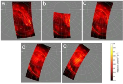
The five composite JIRAM-L images are shown in Fig. 2 . As men- tioned before, all measurements are made in the Juno spin plane, which somewhat limits the spatial coverage compared to UVS. As a consequence, the sector of the Io auroral footprint was not ob- served in any of the JIRAM images during this time interval. Al- though the global structure of the IR auroral emissions appears similar to the ultraviolet, the different spatial resolution and ex- citation processes between the two emissions create remarkable differences. First, auroral structures such as the main emission at longitude beyond 180 ° appear remarkably thin, with a latitudinal width as narrow as ∼100km, comparable with the spatial resolu- tion. Second, what appears as a single main emission arc in the FUV with diffuse equatorward aurora in the 30 °−70° S III sector is
composed of a series of filamentary arcs in JIRAM images 1, 2 and 3. These arcs are best seen in image 1 where as many as 10 arcs structures may be observed, progressively transforming into un- structured emission at lower latitude. They are also visible in the complete dataset ( Mura et al., 2017 ). Polar emissions are ubiqui- tous with no region void of infrared emission, although some of the IR contribution may result from insufficient background sub- traction. Two spots are present near the 0 ° sector embedded into diffuse emission, likely linked to plasma injections. They are still present in the last image, although their brightness is slightly de- creased. Detailed visual inspection and coordinate pointing reveals that they have moved clockwise (in the polar projection) during the 72-min period of observation. Similarly, on the first image two
Table 1
Time and Juno location during the periods of concurrent UVS-JIRAM observations.
Image start (UT) end (UT) altitude (10 3 km) sub-spacecraft resolution ∗(km)
Lat Long UVS JIRAM
1 09:54:24 10:06:42 258 52.9 ° 173 ° 901 61
2 10:09:15 10:17:58 239 54.9 ° 181 ° 834 57
3 10:24:05 10:36:24 214 57.7 ° 191 ° 747 51
4 10:38:56 10:51:14 191 60.7 ° 200 ° 667 45
5 10:54:17 11:06:36 167 64.3 ° 209 ° 583 40
∗ Sub-satellite horizontal resolution
Fig. 1. Five polar orthographic projections from composite images obtained by integrating observations by the UVS instrument over time intervals (see Table 1 ). The color scale is identical for all five images and ranges from 0 to 1 MegaRayleigh. The projections are oriented with the 0 ° S III meridian to the top and System III longitudes
increasing clockwise. The grey zones correspond to the regions not observed by UVS. The latitude circles and meridians are separated by 10 ° and the sun directions at the beginning and end of the images are indicated by the yellow lines. The statistical contours from HST of the main auroral emission and of the Io footprint are shown by the white dotted lines. (For interpretation of the references to color in this figure legend, the reader is referred to the web version of this article.)
Fig. 2. Same as Fig. 1 for the JIRAM-L mosaics. The orientation is the same as in Fig. 1 . The statistical contours of the main emission and the Io footprint are shown by the green lines (from Mura et al., 2017 ). The color scale refers to the radiance measured in the JIRAM-L spectral window (see text). The grey zones correspond to the regions not observed by JIRAM. (For interpretation of the references to color in this figure legend, the reader is referred to the web version of this article.)
Fig. 3. Comparison between the JIRAM co-added images collected between 9:54 and 10:07 UT (a) and the same data smoothed at the UVS spatial resolution (b).
polar spots are seen between 60 ° and 70 ° latitude in the 175 °−190° sector and one is present at 67 ° N and
λ
III= 177 ° In the next twoimages, only the most northern one of the pair is still clearly vis- ible, while the second one has become diffuse and has almost merged into the background emission. The isolated single spot is still present. In the third image, this single spot is no longer ob- served. The last two images barely show a weak feature reminis- cent of the longer-lived spot. Finally, we note that the extended diffuse bright region over most of the polar region in these two images is probably of instrumental origin and should not be inter- preted in terms of physical or chemical processes.
The calculation of synthetic H +3 spectra at different tempera- tures assuming thermodynamic equilibrium ( Dinelli et al., 2017 ) is used to estimate the fraction of emission captured in the spectral window of the JIRAM-L channel. The fraction is then applied to convert the H +3 radiance measured by JIRAM into the total cool- ing rate in the H +3 bands. The fraction is only weakly dependent on temperature, ranging from 20.5% at 800 K to 19.3% at 10 0 0 K. In the following, we adopt a mean value of 20%. The radiance inte- grated over the 3.3–3.6 μm spectral window of the JIRAM-L chan- nel reaches up to 0.5 mW m −2 sr −1 on the filamentary structures of images 1 and 2 along the 155 ° meridian. Based on the 20% scal- ing factor, this corresponds to 2.5 mW m −2 sr −1 for the total H +3 emission.
To facilitate the comparison, the JIRAM images have been smoothed to the same spatial resolution as the UVS images. Since the UVS-JIRAM observations are never exactly simultaneous, an in- stantaneous comparison of the relative projected resolution is not possible. Therefore, a simple boxcar smoothing by a factor of 10 has been applied to the JIRAM images to take into account the fact that JIRAM-L field of view is approximately 10 times sharper than UVS. Fig. 3 shows a comparison of the original co-added JIRAM im- ages collected between 9:54 and 10:07 and the smoothed version. Figs. 4 and 5 present two sets for detailed comparison between the images collected by the two imagers during the first and the third concurrent times intervals. These are the two sets of co- added images offering the best common spatial coverage. The top part shows side-by-side the polar projections of the UVS H 2inten-
sity (a) and the FUV color ratio (b). The wavelength range used to integrate the absorbed H 2 emission is limited to the 123–130 nm
interval to avoid contamination by the wing of the Lyman-
α
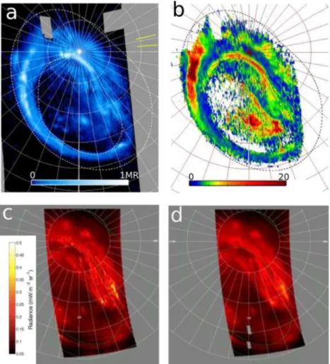
line. The bottom part shows the JIRAM mosaics obtained during the same time interval at the original (c) and the same data smoothed to the UVS spatial resolution (d). The global morphology observed in the two spectral regions is quite similar when compared at the same spatial resolution. As mentioned before, the FUV color ratio is directly related to the energy of the precipitating electrons, asthe harder electrons penetrate deeper into the hydrocarbon layer, causing an increase of the color ratio ( Yung et al., 1982 ). The values range from less than 2 at the Io footprint up to 20 in the bright region close to the 250 ° S III meridian. These numbers are within
the range of values previously observed on HST FUV spectral im- ages of the north aurora ( Gérard et al., 2014 : Gustin et al., 2016 ). The enhancement of the main emission that is quite pronounced in the UVS image near the jovigraphic pole is not observed in ei- ther infrared projection. The color ratio map shows that it is as- sociated with a region of high FUV color ratio (up to 10), corre- sponding to an estimated electron mean energy of 20 0–40 0 keV ( Gérard et al., 2014 ). The drop of the UV intensity along the main emission with decreasing latitudes equatorward of 83 ° N is asso- ciated with a decrease of the color ratio. A brightening of the H +3 emission is seen in the 80 ° N, 155 ° S III sector, a region of moder-
ate UV color ratio. The IR polar spots at
λ
III=190 ° and 197 ° standout more clearly than in the UV. By contrast, the H 2isolated spot
at
λ
III= 178 ° is considerably stronger than the other high-latitudetriangular spot structure between 190 ° and 200 °, which are associ- ated with a color ratio as high as 20 in the center. Globally, these results show a trend for high FUV/IR ratio associated with areas of relatively high color ratio.
Li et al. (2017) analyzed the morphology of the UV diffuse au- rora in parallel with the in situ characteristics of the electron pre- cipitation in the diffuse region measured a couple of hours later near
λ
III=120 °–150 ° They provided evidence that the loss conewas nearly full over energies 0.1–700 keV. Pitch angle scattering into the loss cone is thought to produce diffuse auroral emissions ( Coroniti et al., 1980 ; Bhattracharya et al., 2001; Radioti et al., 2009 ). It is likely caused by whistler mode waves generated as a result of anisotropic electron injections scattering energetic elec- trons. The poleward edge of the latitudinal band of low color ratio (CR <4) between the main emission and the lower latitude emis- sion coincides with the low latitude boundary of the narrow arcs observed in the JIRAM co-added image shown in Figs. 3 and 4 c.
Fig. 5 , based on data collected between 30 and 42 min. later, confirms these conclusions in spite of the more limited UVS spa- tial coverage. Here again, the spot at 69 °N on the 177 ° meridian is still visible, although dimmer, in the FUV and has not signifi- cantly moved in longitude during the time interval. By contrast, it is no longer observable in the H +3 polar map projection. Interest- ingly, in the meantime, the size of the zone with CR >20 associ- ated color ratio has further increased. We also note that the dou- ble arc feature observed by both instruments near 60 ° N at dawn between 190 ° and 210 ° longitude exhibits a remarkable difference in the two spectral bands. In the ultraviolet, the outermost arc is brighter than the inner one (panel a), while the relative intensity
Fig. 4. Auroral projections of co-added images between 9:54:24 and 10:06:42. (a): FUV H 2 emission; b: FUV color ratio; c: native resolution JIRAM image; d: smoothed
JIRAM image. The 0 ° S III meridian is oriented to the top, 90 ° to the right and 180 ° to the bottom of the page.
of the two arcs is reversed in the infrared (panels c and d). Panel b indicates that a higher color ratio between 3.8 and 8 (harder elec- tron precipitation) is associated with the outer arc segment than with the inner one which remains less than 2. It is reasonable to assume that the energetic electrons producing aurora with a high color ratio spot deposit an increasingly large fraction of their en- ergy below the homopause where H +3 ions are rapidly lost by their chemical reaction with methane:
H+3+CH4→CH+5 +H2,
which efficiently prevents H +3ions from radiating below the ho- mopause where the methane density rapidly increases with depth. This point will be further illustrated in the next section.
Comparisons between UV and IR polar emissions become more difficult during the subsequent time intervals when the JIRAM images became increasingly affected by instrumental background noise. However, the spot near the pole at 70 ° N is clearly observed in the UV and IR.
5. Intensity distribution
A more detailed comparison between the H 2 and H +3 emis-
sions is obtained by comparing intensities in two simultaneous im- age cuts starting from the barycenter of the main emission. Fig. 6 shows the location of two cuts made through the first compos- ite JIRAM and UVS images collected between 9:54 and 10:07. Both cuts originate from the position of the barycenter (74 °N,
λ
III=185 °)of the statistical ‘main FUV oval’ determined from Hubble FUV im- ages as described by Grodent et al., 2003a ).
5.1. Comparativeintensitydistribution
To increase the signal to noise ratio, the two cuts are made over a width of about 400 km (center ± 200km), corresponding to the width of the line in the JIRAM cut of Fig. 6 . To eliminate differences caused by the different spatial resolution of the two instruments, the cut through the H +3 image is made on the smoothed version of the JIRAM image shown in Fig. 4 d. The unabsorbed H 2 emission
rate has been converted from kiloRayleigh (10 9 photons cm −2s −1
in 4
π
steradians) into radiance units (mW m −2 sr −1) to facilitate direct comparison.Similarities and differences are readily observed when compar- ing the two intensity curves in Figs. 7 and 8 . In the FUV, cut #1 successively crosses a polar region of diffuse emission, fol- lowed by a relatively dark region, a bright arc that is part of the main emission and a region of diffuse equatorward emission. The three UV emission regions correspond to the intensity peaks lo- cated 9 × 10³km, 1.35 × 10⁴ and 1.9 × 10⁴km from the line origin
in Fig. 7 . A peak in the H +3 emission is co-located with the FUV peak of the main emission, but the other two FUV maxima show no enhanced infrared counterpart. Inversely, the H +3 emission peak at 1.7 × 10⁴km corresponds to a dip in the H
2 brightness. We note
that on the original JIRAM image, the arc structure is consider- ably more complex than in the FUV. To provide further insight into the IR-UV relationship, the bottom panel shows the measured FUV color ratio (CR) along the cut. The regions between 5 × 10³
and 6 × 10³km, 1 × 10⁴and 1.2 × 10⁴km, 1.6 × 10⁴and 1.8 × 10⁴km
which show CR minima as low as 2 are associated with high IR/UV ratios. These observations indicate that the H +3 emission is
Fig. 5. Same as Fig. 4 for projections of co-added images between 10:24 and 10:36.
Fig. 6. The two lines on both images indicate the location of the intensity cuts from the ‘oval center’ through the co-added UVS and native JIRAM images obtained between 9:54 and 10:07 UT.
relatively bright in regions of softer electron precipitation, in agreement with model calculations ( Tao et al., 2011 ). Inversely, the main emission peak at 1.33 × 10 4km shows the lowest IR/UV ratio
and the highest color ratio (8.5) along the cut. The infrared emis- sion is significantly enhanced in this region relative to the FUV, in agreement with the drop in mean electron energy measured in situ by JADE and JEDI during the later Juno crossing of this zone ( Li et al., 2017 ; Fig. 2 ). Additionally, increased H +3 thermospheric temperatures were observed in this sector by Dinelli et al. (2017) . These conditions favor the production of H +3photons from higher
altitudes than in the other regions. The other two ultraviolet peaks at 9 × 10³ and 1.9 × 10⁴km are also associated with the two sec-
ondary maxima in the color ratio.
Fig. 8 shows a similar comparison between the FUV and in- frared radiances along cut #2. In this case, the crossing of the main emission is seen at a distance close to 9.2 × 10 3km from the
barycenter in both wavelengths. The peak is more structured in the H +3 emission. The bright FUV main emission has dropped in bright- ness by more than a factor of 2 in comparison with cut #1, while the corresponding H +3 maximum is only 24% less. Compared to the
Fig. 7. Comparison of the intensity cut #1 from the oval barycenter through the composite JIRAM and UVS images in Fig. 4 . The blue curve shows the total H 2 and
the red line represents the cut through the smoothed JIRAM image, both expressed in radiance units. The bottom panel is the FUV color ratio measured along the cut shown in Fig. 6 . (For interpretation of the references to color in this figure legend, the reader is referred to the web version of this article.)
Fig. 8. Same as Fig. 7 for radial cut #2.
first cut, cut #2 crosses a region of lower color ratio in the region of the main emission. A secondary peak in both emissions is co- located near 1.25 × 10⁴km. By contrast, the infrared emission pole-
ward of the main arc between 5 and 7 × 10 3km corresponds to a
low intensity in the H 2 emission. The regions where CR <2 near
6 × 10³, 1.4 × 10⁴ and 2.0 × 10⁴ are coincident with high IR/UV in-
tensity ratios. Conversely, the bright UV peak at 9 × 10 3km is as-
sociated with the lowest IR/UV ratio and corresponds to the re- gion of the highest color ratio ∼4.9. This second example confirms the association between regions of high FUV color ratio and harder electron precipitation.
5.2. H +3 radiative cooling
The H +3 temperatures can be derived from the relative inten- sity of the emission lines in the auroral H +3 spectrum assuming thermodynamic equilibrium (LTE). The fraction of H +3 molecules in LTE remains close to 100% in the Jovian high-latitude atmo- sphere below 10 0 0–20 0 0 km ( Tao et al., 2011 ). The LTE assumption is therefore increasingly valid when the electron initial energy in- creases, with significant departures only predicted for electron en- ergies below a few keV. Several measurements show that tempera- ture is variable in space and time and remains within the range of 70 0–10 0 0 K ( Lam et al., 1997 ), 900–1250 K ( Stallard et al., 2002 ), 1170 ± 75K ( Raynaud et al., 2004 ). Lystrup et al., (2008) deter- mined exospheric temperatures of 1450 K from limb observations. During the PJ1 Juno orbital phase, Dinelli et al. (2017) mapped si- multaneously the H +3 temperature and column density in the north aurora from the line ratios in the 35. μm region used on the JIRAM infrared spectral imager. They derived temperature values ranging from about 800 K inside the main emission up to 950 K ± 100K equatorward of the main statistical UV oval in the kink region. These observations indicated a complex spatial relationship be- tween the H +3 column density and temperature in the north aurora. In particular, they found that one side of the main emission shows higher H +3column densities and lower temperatures than the other side. These spatial differences partly explain the wide scatter and the hint of anti-correlation in the temperature-column density plot obtained by Adriani et al. (2017a) from the PJ1 spectral images.
The results illustrated in Figs. 7 and 8 provide a unique oppor- tunity to estimate the importance of H +3 radiative cooling to space and a direct comparison of the ultraviolet H 2 emission rate with
the H +3 radiance. An electron precipitation of 1 mW m −2 generates approximately 10 kR (1.28 × 10mW m −2 sr −1) of total H 2 emission
from the B and C singlet states over a wide range of initial elec- tron energies ( Gérard and Singh, 1982; Waite et al., 1983 ). There- fore, the H 2UV intensity spatial distribution maps the precipitated
electron energy flux in the auroral regions. Waite et al. (1983) es- timated the fraction of the precipitated energy leading to atmo- spheric heating as 11% for direct collisional heating and close to ∼50% for total heating, including heat from H 2+, electron heating
and vibrational energy. Joule heating, particle drag and compres- sional heating provide an additional, probably much larger, contri- bution to the thermal balance of the upper auroral atmosphere. Similarly, heat conduction, advection and radiation by hydrocar- bons near and below the homopause plays a key role in cooling the auroral thermosphere. Nevertheless, it is important to use the opportunity of concurrent UV and infrared measurements for the determination of the amount of auroral energy direct input from the electrons and of the heat leaving the Jovian atmosphere in the form of H +3 radiation. Since the relative brightness of the H 2 UV
and H +3 IR emissions varies along the cuts, the fraction of the au- roral energy provided by particle heating that is radiated by H +3 varies accordingly. However, to quantify this fraction, we consider values related to bright arcs prominent in Fig. 7 and 8 and values integrated along the cuts.
We start from the comparison between the radiance of the H 2
emission and the co-located total H +3 emission in bright arcs. These conditions correspond to the lowest value of the IR/UV ratio along the cuts made through Figs. 7 and 8 . As an example, cut #1 shows a maximum value of 0.62 mW m −2sr −1(580 kR) of unabsorbed H 2
radiance at a distance of 1.35 × 10⁴km from the auroral barycenter
(the origin of the distance scale). The corresponding total H +3 in- frared power is 1.1 mW m −2 sr −1, that is 1.8 time the power emit- ted in the H 2 ultraviolet emission. Using the conversion factor of
10 kR of H 2emission per incident mW m −2electron precipitation,
mated ∼58 mW m −2. The fractional cooling efficiency by H +3 radi- ation relative to the electron heating is thus equal to 0.48.
Similarly for the second cut shown in Fig. 8 , the common peak 9 × 10³km from the barycenter reaches 0.35 mW m −2 sr −1 (270
kR) in the ultraviolet and 0.25 mW m −2 sr −1 in the JIRAM chan- nel bandpass, corresponding to a ratio of the total IR/UV radiance equal to 3.6. The corresponding H +3 cooling efficiency is 1.2 time the electron heating rate. These values relative to bright arcs cor- respond to the lowest IR/UV brightness ratio along the cuts and therefore to the smallest fraction of H +3 cooling fractions.
When averaged over the full length of the radial cut, the ratios of the IR/UV radiances are 3.4 and 7.5 for cuts 1 and 2 respectively, significantly higher than in the bright arcs. The average H +3 cooling efficiency relative to heating by electrons is then 1.1 for cut #1 and 2.4 for cut #2. These values, together with the curves in Figs. 7 and 8 , indicate that the energy that is dissipated through the H +3 radi- ation is on the same order of magnitude as the particle heating rate but is also spatially quite variable. It is however important to note that Joule heating and ion drag are probably the dominant auroral heat sources, which explains that cooling by H +3 emission to space may significantly exceed the auroral electron heating rate. Additionally, heat loss processes other than H +3 emission such as hydrocarbon thermal emission, vertical conduction and advection also play an important role in the global heat budget ( Melin et al., 2006; Majeed et al., 2009 ).
5.3.Comparisonwithinsituelectronfluxmeasurements
Juno crossed the magnetic field lines threading the north aurora approximately two hours after the UVS and JIRAM images were collected. Early results collected with the particle detectors in both polar regions during the PJ1 phase of the Juno orbit have been summarized by Connerney et al. (2017) . They indicated that en- ergy depositions as large as 80 mW m −2 were measured by JEDI in the loss cone during PJ1 in the north aurora. Further analy- ses have provided a comprehensive picture of the evolution of the electron energy spectra, pitch angle distributions and fluxes mea- sured during the Juno PJ1 crossing of the north polar regions by JADE in the 0.1 to 100 keV range ( Szalay et al., 2017; Allegrini et al., 2017; Ebert et al., 2017; Li et al., 2017 ) and by JEDI from 25 keV to 800 keV ( Mauk et al., 2017a, 2017b ). This energy was carried by non-beaming diffuse precipitation, contrary to the Earth where intense aurora is generally associated with discrete auroral pro- cesses such as peaked electron beams known as inverted-V struc- tures. Both instruments showed no signature of narrowly peaked electron distribution during the encounter. However, broad mono- tonic energy distributions were identified that were attributed to a stochastic acceleration process generating the most intense auroral emissions ( Mauk et al., 2017b ). A detailed correspondence between the filamentary structures observed with JIRAM in the 0 ° to 160 ° longitude sector and those measured in situ in the same sector ∼2 h. later is not possible. However, an indication may be obtained by comparing the spatial frequency of the multiple arcs observed by JIRAM in the sector of the two intensity cut with those measured in the downgoing electron fluxes in the loss cone. For this pur- pose, we note that 5 to 7 arc filaments were detected in the JIRAM images along the radial cut shown in Fig. 7 . They were possibly as- sociated with a succession of alternatively upward and downward current paths by Mura et al. (2017) .
During the crossing of the middle plasma sheet between 12:10 and 12:13, roughly magnetically mapping to the same region as cut #1, the JADE electron detectors encountered several bursts of mostly upward going electrons with energies up to about a few tens of keV. The JEDI instrument did not have the time resolution to resolve each of these structures, but downward fluxes of ener- getic electron ( >165 keV) in the loss cone about 8 mW m −2 were
measured during this period ( Mauk et al., 2017a ), with values as high as 200 mW m −2 equatorward. This energy flux would gener- ate total H 2 emission rates on the order of 80 kR and 2 MR re-
spectively, in reasonable agreement with the subsequent FUV ob- servations, considering the 2-hour delay between the two sets of observations. However, as illustrated by Bonfond et al. (2017a) , the uncertainties on the structure of magnetic field in the vicinity of the planet limits the accuracy of the magnetic mapping from Juno to the ionosphere. This is especially the case in the region of the magnetic anomaly where the Juno measurements and the intensity cuts described before were made.
6. Discussion and conclusions
Juno’s FUV and IR imaging spectrographs captured images of the Jovian northern aurora from a unique vantage point above the poles and providing the first simultaneous global view of the aurora, including the nightside sector. The unabsorbed H 2
Werner and Lyman bands measured with UVS directly map the precipitated electron energy flux. By contrast, the brightness of the H +3 bands measured by the JIRAM-L depends on the H +3 col- umn density and the atmospheric temperature within the emit- ting region. The global morphological features observed in the two emissions are quite similar as may be expected from the common source of electron energy input. However, important dif- ferences have been observed in the relative brightness of differ- ent features in the infrared and ultraviolet in simultaneous im- ages. These may be explained by some differences in the alti- tude distribution of the H 2 vol emission rate and the H +3 ion den-
sity distribution. For example, we showed that regions associated with a low FUV color ratio (and thus softer electron precipitation) are generally brighter in the infrared relative to their ultraviolet counterparts.
Differences observed in the detailed comparison of the bright- ness in the two spectral domains along radial cuts are quite pro- nounced. Even though the production rate of H +3 ions closely mim- ics the excitation of H 2by energetic electrons, three factors induce
differences in the intensity ratio between the two emissions. First, if a significant fraction of the H +3 column is created near or below the homopause, the fast reaction with methane will considerably reduce their contribution of the column emission rate. This ap- pears to be the case in Figs. 4 and 5 and 7 and 8 where the bright FUV regions relative to the H +3 are generally coincident with an en- hanced color ratio. Second, the H +3 temperature distribution in the polar regions is not horizontally constant, which implies that some of the infrared emission is not only controlled by the amount of H +3 ions, but also by the thermospheric temperature distribution. Ear- lier studies have indicated that the H +3 column density and tem- peratures show some degree of anticorrelation ( Lam et al., 1997; Adriani et al., 2017a ). The comparison of the H +3 density and tem- perature maps deduced from the JIRAM spectra collected during PJ1 by Dinelli et al. (2017) indicates that the regions of enhanced temperature did not coincide with those of enhanced H +3density. By contrast, H +3 ion transport is expected to play a minor role since their chemical lifetime is expected to be too short to allow them to travel over significant distances. Adopting a horizontal drift ve- locity between 10 and 50 m s −1 and a H +3lifetime of 4–40 s near the emission peak, Radioti et al., (2013) estimated that the ions move by a distance between 40 m and 2 km. These small values imply that horizontal transport is negligible in restructuring the auroral H +3morphology. The very narrow arc structures observed with JIRAM and their stability over several tens of minutes con- firms that they are indeed not appreciably blurred by horizontal transport.
The H +3cooling rates relative to the particle heat input de- termined in this study vary from 0.48 in the bright main
emission arc to 2.4 when averaged over the second radial cut. They may be compared with the 0.47 and 0.83 values derived by Melin et al. (2006) whose estimates were obtained by comparing ground-based H +3measurements during an auroral heating event with the particle heating rate. The auroral particle flux was esti- mated from the H +3 radiance using an empirical relationship be- tween the H +3 column density and the incident auroral electron power. A first difference is that in this study we determine the electron energy input directly from simultaneous measurements of the H 2 and H +3co-located emission rates. Second, the values deter-
mined here refer to a specific region of the Jovian aurora, namely the longitude sector of the magnetic anomaly ( Grodent et al., 2008 ). We also note that these values are directly dependent on the absolute calibration of the two instruments and the subtrac- tion of the background noise in the JIRAM and UVS images. The thermospheric GCM simulation ( Majeed et al., 2009 ) also indicated that particle heating is not the major high latitude heat source in the thermosphere.
It is however important to stress that Joule and ion drag heat- ing and adiabatic compression are probably the globally domi- nant auroral heat sources at pressures above the homopause (P <1 μbar) in the main emission as calculated by Majeed et al. (2009) . This explains that cooling by H +3emission to space may glob- ally exceed the electron precipitation heating rate. Additionally, heat loss processes other than H +3emission such as hydrocarbon thermal emission, vertical conduction and advection also play an important role in the global heat budget ( Melin et al., 2006 ; Majeed et al., 2009 ). Further modeling studies using an extended database of concurrent observations will indicate whether sig- nificant variations are observed in the role of the H +3radiation in the local and global auroral thermal budget. If confirmed on a permanent and global scale, our results suggest the thermo- static role of H +3radiation may not be as dominant as previously thought.
Finally, the multiple arcs observed with JIRAM appear compati- ble with the structure measured in the JADE upward electron flux when Juno flew over the same area about two hours later. How- ever, mapping the electron flux measured in situ to the ionosphere is limited by the knowledge of the magnetic field in the vicinity of the planet. In addition, the detailed morphology may have changed during this time interval, which prevents establishing a point-to- point spatial correspondence.
In summary, this first study of global simultaneous images of the H 2 FUV and H +3infrared emission leads to the following con-
clusions:
– the morphology of the infrared and ultraviolet auroral emis- sions are globally similar
– the higher spatial resolution of the JIRAM images shows the presence of multiple arcs in the region of the magnetic anomaly – these structures are compatible with those measured in situ in the flux of downward electrons measured when Juno crossed the zone magnetically mapping to the same region
– differences in the relative intensities of the two emissions are ubiquitous
– the ratio of the H +3 radiance to the H 2 intensity decreases in
regions characterized by a high color ratio, that is which are submitted to harder electron precipitation
– this feature is likely explained by the rapid loss of H +3 ions pro- duced near or below the methane homopause where they are rapidly destroyed by reaction with methane
– the atmospheric cooling rate by H +3 thermal radiation is of the same order of magnitude as the particle heating rate es- timated from the H 2 intensity, but shows significant spatial
variations.
Acknowledgements
The JIRAM project has been funded by the Italian Space Agency under contract number 2016-32123-H.0 . The Juno-UVS instru- ment was funded under contracts NAS703001TONMO710962 and NNM06AA75C to NASA. J.-C.G., B.B., D.G., and A.R. acknowledge support from the PRODEX program managed by ESA in collabora- tion with the Belgian Federal Science Policy Office (BELSPO).
References
Adriani, A., et al., 2017a. Preliminary results from the JIRAM auroral observations taken during the first Juno orbit: 2—Analysis of the Jupiter southern H +
3 emis-
sions and comparison with the north aurora. Geophys. Res. Lett. doi: 10.1002/ 2017GL072905 .
Adriani, A. , et al. , 2017b. JIRAM, the Jovian infrared Auroral Mapper. Space Sci. Rev. 213, 393–446 .
Allegrini, F., et al., 2017. Electron beams and loss cones in the auroral regions of Jupiter. Geophys. Res. Lett. 44, 7131–7139. doi: 10.1002/2017GL073180 . Badman, S.V., 2014. Auroral processes at the giant planets: energy deposition,
emission mechanisms, morphology and spectra. Space Sci. Rev. doi: 10.1007/ s11214-014-0042-x .
Bagenal, F. , et al. , 2017. Magnetospheric science objectives of the Juno mission. Space Sci. Rev. 213, 219–287 .
Baron, R. , Joseph, R.D. , Owen, T. , Tennyson, J. , Miller, S. , Ballester, G.E. , 1991. Imaging Jupiter’s aurorae from H +
3 emissions in the 3–4μm band. Nature 353, 539–542 .
Bhardwaj, A. , Gladstone, G.R. , 20 0 0. Auroral emissions of the giant planets. Rev. Geo- phys. 38 (3), 295–353 .
Bhattacharya, B. , Thorne, R.M. , Williams, D.J. , 2001. On the energy source for diffuse Jovian auroral emissivity. Geophys. Res. Lett. 28 (14), 2751–2754 .
Bolton, S., Levin, S., Bagenal, F., 2017. Juno’s first glimpse of Jupiter’s complexity. Geophys. Res. Lett. 44, 7663–7667. doi: 10.1002/2017GL074118 .
Bonfond, B., Grodent, D., Gérard, J.-C., Radioti, A., Dols, V., Delamere, P. A., Clarke, J. T., 2009. The Io UV footprint: Location, inter-spot distances and tail vertical ex- tent. J. Geophys. Res. 114, A07224. doi: 10.1029/2009JA014312 .
Bonfond, B., Grodent, D, Badman, S.V., Gérard, J.-C., Radioti, A., 2016. Dynamics of the flares in the active polar region of Jupiter. Geophys. Res. Lett. 43, 11,963– 11,970. doi: 10.1002/2016GL071757 .
Bonfond, B., et al., 2017a. Morphology of the UV aurorae Jupiter during Juno’s first perijove observations. Geophys. Res. Lett. 4 4, 4 463–4 471. doi: 10.1002/ 2017GL073114 .
Bonfond, B, Saur, J., Grodent, D., Badman, S.V., Bisikalo, D., Shematovich, V., Gérard, J.-C., Radioti, A., 2017b. The tails of the satellite auroral footprints at Jupiter. J. Geophys. Res. Space Phys. 122 (A7). doi: 10.1002/2017JA024370 . Clarke, J.T. , Grodent, D. , Cowley, S.W.H. , Bunce, E.J. , Zarka, P. , Connerney, J.E.P. ,
Satoh, T. , 2004. Jupiter’s aurora, in Jupiter, The Planet, Satellites and Magne- tosphere. Cambridge Univ. Press, Cambridge, U. K., pp. 639–670 .
Connerney, J.E.P. , 1992. Doing more with Jupiter’s magnetic field. In: Rucker, H.O., Bauer, S.J. (Eds.), Planetary Radio Emissions III. Austrian Academy of Sciences Press, Austrian Academy of Science, Austria, pp. 13–33 .
Connerney, J.E.P. , Satoh, T. , 20 0 0. The H +
3 ion: A remote diagnostic of the Jovian
magnetosphere. Phil. Trans. R. Soc. Lond. A 358, 2471–2483 .
Connerney, J.E.P. , Baron, R. , Satoh, T. , Owen, T. , 1993. Images of excited H + 3 at the
foot of the Io flux tube in Jupiter’s atmosphere. Science 262, 1035–1038 . Connerney, J.E.P. , et al. , 2017. Jupiter’s magnetosphere and aurorae observed by the
Juno spacecraft during its first polar orbits. Science 356 (6340), 826–832 . Coroniti, F.V. , Scarf, F.L. , Kennel, C.F. , Kurth, W.S. , Gurnett, D.A. , 1980. Detection of
Jovian whistler mode chorus: Implications for the Io torus aurora. Geophys. Res. Lett. 7 (1), 45–48 .
Cowley, S.W.H. , Bunce, E.J. , 2001. Origin of the main auroral oval in Jupiter’s coupled magnetosphere–ionosphere system. Planet. Space Sci. 49 (10), 1067–1088 . Cowley, S.W.H. , Bunce, E.J. , Nichols, J.D. , 2003. Origins of Jupiter’s main oval auroral
emissions. J. Geophys. Res 108 (A4) .
Dinelli, B.M., et al., 2017. Preliminary JIRAM results from Juno polar observations: 1. Methodology and analysis applied to the Jovian northern polar region. Geophys. Res. Lett. 44, 4625–4632. doi: 10.1002/2017GL072929 .
Dols, V. , Gérard , Paresce, J.-C. , Prangé, F. , Vidal-Madjar, R. , 1992. A. Ultraviolet imag- ing of the Jovian aurora with the Hubble Space Telescope. Geophys. Res. Lett. 19, 1803–1806 .
Drossart, P. , Maillard, J.P. , Caldwell, J. , Kim, S.J. , Watson, J.K.G. , Majewski, W.A. , ... , Waite, J.H. , 1989. Detection of H +
3 on Jupiter. Nature 340 (6234), 539–541 .
Drossart, P., Bézard, B., Atreya, S.K., Bishop, J., Waite Jr., J.H., Boice, D., 1993. Thermal profiles in the auroral regions of Jupiter. J. Geophys. Res. 98 (E10), 18803–18811. doi: 10.1029/93JE01801 .
Dumont, M., Grodent, D., Radioti, A., Bonfond, B., Gérard, J.-C., 2015. Jupiter’s equa- torward auroral features: Possible signatures of magnetospheric injections. J. Geophys. Res. 119. doi: 10.1002/2014JA020527 , 10,068–10,077 .
Ebert, R.W., Allegrini, F., Bagenal, F., Bolton, S.J., Connerney, J.E.P., Clark, G., …, Wil- son, R.J., 2017. Spatial distribution and properties of 0.1–100keV electrons in Jupiter’s polar auroral region. Geophys. Res. Lett. 44, 9199–9207. doi: 10.1002/ 2017GL075106 .
Gérard, J.-C., Singh, V., 1982. A model of energy deposition of energetic electrons and EUV emission in the Jovian and Saturnian atmospheres and implications. J. Geophys. Res. 87 (A6), 4525–4532. doi: 10.1029/JA087iA06p04525 .
Gérard, J.-C. , Dols, V. , Paresce, F. , Prangé, R. , 1993. Morphology and time variation of the Jovian far UV aurora: Hubble Space Telescope observations. J. Geophys. Res. 98, 18793–18801 .
Gérard, J.-C. , et al. , 1994. A remarkable auroral event on Jupiter observed in the ultraviolet with the Hubble Space Telescope. Science 1675–1678 .
Gérard, J.C. , et al. , 2014. Mapping the electron energy in Jupiter’s aurora: Hubble spectral observations. J. Geophys. Res. 119 (11), 9072–9088 .
Gladstone, G.R., et al., 2017a. Juno-UVS approach observations of Jupiter’s auroras. Geophys. Res. Lett. 44, 7668–7675. doi: 10.1002/2017GL073377 .
Gladstone, G.R. , et al. , 2017b. The ultraviolet spectrograph on NASA’s Juno mission. Space Sci. Rev. 213, 447–473 .
Grodent, D., Clarke, J.T., Kim, J., Waite Jr., J.H., Cowley, S.W.H., 2003a. Jupiter’s main auroral oval observed with HST- STIS. J. Geophys. Res. 108, 1389. doi: 10.1029/ 20 03JA0 09921 .
Grodent, D., Clarke, J.T., Waite, J.H., Cowley, S.W.H., Gérard, J.-C., Kim, J., 2003b. Jupiter’s polar auroral emissions. J. Geophys. Res. 108, 1366. doi: 10.1029/ 20 03JA010 017 .
Grodent, D. , Bonfond, B. , Gérard, J.-C. , Radioti, A. , Gustin, J. , Clarke, J.T. , ... , Conner- ney, J.E. , 2008. Auroral evidence of a localized magnetic anomaly in Jupiter’s northern hemisphere. J. Geophys. Res 113 (A9) .
Grodent, D. , 2015. A brief review of ultraviolet auroral emissions on giant planets. Space Sci. Rev. 187 (1-4), 23–50 .
Greathouse, T.K. , et al. , 2013. Performance results from in-flight commissioning of the Juno Ultraviolet Spectrograph (Juno-UVS). In: Siegmund, O.H. (Ed.), UV, X-Ray, and Gamma-Ray Space Instrumentation for Astronomy XVIII, 8859 SPIE proceedings .
Gustin, J. , D. , Ray, L.C. , Bonfond, B. , Bunce, E.J. , Nichols, J.D. , Ozak, N. , 2016. Char- acteristics of north Jovian aurora from STIS FUV spectral images. Icarus 268, 215–241 .
Hess, S.L.G., Delamere, P., Dols, V., Bonfond, B., Swift, D., 2010. Power transmission and particle acceleration along the Io flux tube. J. Geophys. Res. 115, A06205. doi: 10.1029/2009JA014928 .
Hill, T.W., 2001. The Jovian auroral oval. J. Geophys. Res. 106 (A5), 8101–8107. doi: 10. 1029/20 0 0JA0 0 0302 .
Kim, Y.H., Fox, J.L., Porter, H.S., 1992. Densities and vibrational distribution of H + 3
in the Jovian auroral ionosphere. J. Geophys. Res. 97, 6093–6101. doi: 10.1029/ 92JE00454 .
Lam, H.A. , Achilleos, N. , Miller, S. , Tennyson, J. , Trafton, L.M. , Geballe, T.R. , Ballester, G.E. , 1997. A baseline spectroscopic study of the infrared auroras of Jupiter. Icarus 127 (2), 379–393 .
Li, W., et al., 2017. Understanding the origin of Jupiter’s diffuse aurora using Juno’s first perijove observations. Geophys. Res. Lett. doi: 10.1002/2017GL075545 . Lystrup, M. B., Miller, S., Dello N., R., Vervack, R. J., Stallard, T., 2008. First vertical
ion density profile in Jupiter’s upper atmosphere: Direct observations using the Keck II Telescope. ApJ 677, 790–797. doi: 10.1086/529509 .
Majeed, T., Waite, J.H., Bougher, S.W., Gladstone, G.R., 2009. Processes of auroral thermal structure at Jupiter: Analysis of multispectral temperature observations with the Jupiter Thermosphere General Circulation Model. J. Geophys. Res. 114, E07005. doi: 10.1029/2008JE003194 .
Mauk, B.H. , Clarke, J.T. , Grodent, D. , Waite Jr., J.H. , Paranicas, C.P. , Williams, D.J. , 2002. Transient aurora on Jupiter from injections of magnetospheric electrons. Nature 415, 10 03–10 05 .
Mauk, B.H., et al., 2017a. Juno observations of energetic charged particles over Jupiter’s polar regions: Analysis of monodirectional and bidirectional electron beams. Geophys. Res. Lett. 44, 4410–4418. doi: 10.1002/2016GL072286 . Mauk, B.H , et al. , 2017b. Discrete and broadband electron acceleration in Jupiter’s
powerful aurora. Nature 549, 66–69 .
Melin, H. , Miller, S. , Stallard, T. , Smith, C. , Grodent, D. , 2006. Estimated energy bal- ance in the jovian upper atmosphere during an auroral heating event. Icarus 181 (1), 256–265 .
Mura, A., et al., 2017. Infrared observations of Jovian aurora from Juno’s first or- bits: Main oval and satellite footprints. Geophys. Res. Lett. 44, 5308–5316. doi: 10.1002/2017GL072954 .
Nichols, J.D. , Clarke, J.T. , Gérard, J.C. , Grodent, D. , Hansen, K.C. , 2009. Variation of different com ponents of Jupiter’s auroral emission. J. Geophys. Res. 114 (A6) . Radioti, A., Tomás, A.T., Grodent, D., Gérard, J.-C., Gustin, J., Bonfond, B., Krupp, N.,
Woch, J., Menietti, J.D., 2009. Equatorward diffuse auroral emissions at Jupiter: simultaneous HST and Galileo observations. Geophys. Res. Lett. 36, L07101. doi: 10.1029/2009GL037857 .
Radioti, A., Lystrup, M., Bonfond, B., Grodent, D., Gérard, J.-C., 2013. Jupiter’s aurora in ultraviolet and infrared: Simultaneous observations with the Hubble Space Telescope and the NASA Infrared Telescope Facility. J. Geophys. Res. 118, 2286– 2295. doi: 10.1002/jgra.50245 .
Raynaud, E., Lellouch, E., Maillard, J.-P., Gladstone, G.R., Waite, J.H., Bézard, B., Drossart, P., Fouchet, T., 2004. Spectro-imaging observations of Jupiter’s 2- μm auroral emission. I. H +
3 distribution and temperature. Icarus 171, 133–152.
doi: 10.1016/j.icarus.2004.04.020 .
Sandel, B.R. , et al. , 1979. Extreme ultraviolet observations from Voyager 2 encounter with Jupiter. Science 962–966 .
Satoh, T. , Connerney, J.E.P. , Baron, R.L. , 1996. Emission source model of Jupiter’s H + 3
aurorae: A generalized inverse analysis of images. Icarus 122, 1–23 . Satoh, T., Connerney, J.E.P., 1999. Jupiter’s H +
3 emissions viewed in corrected Jovi-
magnetic coordinates. Icarus 141, 236–252. doi: 10.1006/icar.1999.6173 . Stallard, T., Miller, S., Millward, G., Joseph, R.D., 2002. On the dynamics of the Jovian
ionosphere and thermosphere. II. The measurement of H +
3 vibrational tempera-
ture, column density, and total emission. Icarus 156, 498–514. doi: 10.1006/icar. 2001.6793 .
Stallard, T.S., Miller, S., Cowley, S.W.H., Bunce, E.J., 2003. Jupiter’s polar ionospheric flows: Measured intensity and velocity variations poleward of the main auroral oval. Geophys. Res. Lett. 30 (5), 1221. doi: 10.1029/2002GL016031 .
Stallard, T.S. , et al. , 2016. Stability within Jupiter’s polar auroral ‘Swirl region’ over moderate timescales. Icarus 268, 144–155 .
Szalay, J.R. , et al. , 2017. Plasma measurements in the Jovian polar region with Juno/JADE. Geophys. Res. Lett. 44, 7122–7130 .
Tao, C. , Badman, S.V. , Fujimoto, M. , 2011. UV and IR auroral emission model for the outer planets: Jupiter and Saturn comparison. Icarus 213, 581–592 .
Trafton, L. , Lester, D.F. , Thompson, K.L. , 1989. Unidentified emission lines in Jupiter’s northern and southern 2 μm aurorae. Astrophys. J. 343, L73–L76 .
Waite, J.H. , et al. , 1983. Electron precipitation and related aeronomy of the Jovian thermosphere and ionosphere. J. Geophys. Res. 88, 6143–6163 .
Waite Jr, J.H. , Gladstone, G.R. , Lewis, W.S. , Goldstein, R. , 2001. An auroral flare at Jupiter. Nature 410 (6830), 787–789 .
Yung, Y.L., Gladstone, G.R., Chang, K.M., Ajello, J.M., Srivastava, S.K., 1982. H 2 fluores-
cence spectrum from 1200 to 1700 ˚A by electron impact: Laboratory study and application to Jovian aurora. Astrophys. J. 254, L65–L69. doi: 10.1086/183757 .