HAL Id: hal-01406115
https://hal.inria.fr/hal-01406115
Submitted on 2 Dec 2016
HAL is a multi-disciplinary open access
archive for the deposit and dissemination of
sci-entific research documents, whether they are
pub-lished or not. The documents may come from
teaching and research institutions in France or
L’archive ouverte pluridisciplinaire HAL, est
destinée au dépôt et à la diffusion de documents
scientifiques de niveau recherche, publiés ou non,
émanant des établissements d’enseignement et de
recherche français ou étrangers, des laboratoires
A Look-Ahead Simulation Algorithm for DBN Models of
Biochemical Pathways
Sucheendra Palaniappan, Matthieu Pichené, Grégory Batt, Eric Fabre, Blaise
Genest
To cite this version:
Sucheendra Palaniappan, Matthieu Pichené, Grégory Batt, Eric Fabre, Blaise Genest. A Look-Ahead
Simulation Algorithm for DBN Models of Biochemical Pathways. Hybrid Systems Biology, 5th
Inter-national Workshop, HSB 2016, Oct 2016, Grenoble, France. pp.3-15, �10.1007/978-3-319-47151-8_1�.
�hal-01406115�
A Look-ahead Simulation Algorithm for
DBN Models of Biochemical Pathways
Sucheendra K. Palaniappan1,2, Matthieu Pichen´e1, Gregory Batt2, Eric Fabre1, and
Blaise Genest3
1
INRIA, Campus de Beaulieu, Rennes, France
2
INRIA Saclay - Ile de France, Palaiseau, France
3
CNRS, IRISA, Rennes, France
Abstract. Dynamic Bayesian Networks (DBNs) have been proposed [16] as an efficient abstraction formalism of biochemical models. They have been shown to approximate well the dynamics of biochemical models, while offering improved efficiency for their analysis [17,18]. In this paper, we compare different represen-tations and simulation schemes on these DBNs, testing their efficiency and accu-racy as abstractions of biological pathways. When generating these DBNs, many configurations are never explored by the underlying dynamics of the biological systems. This can be used to obtain sparse representations to store and analyze DBNs in a compact way. On the other hand, when simulating these DBNs, singu-larconfigurations may be encountered, that is configurations from where no tran-sition probability is defined. This makes simulation more complex. We initially evaluate two simple strategies for dealing with singularities: First, re-sampling simulations visiting singular configurations; second filling up uniformly these singular transition probabilities. We show that both these approaches are error prone. Next, we propose a new algorithm which samples only those configura-tions that avoid singularities by using a look-ahead strategy. Experiments show that this approach is the most accurate while having a reasonable run time.
1
Introduction
Biological pathway systems are usually modeled by a network of reactions. Their dy-namics is governed by mathematical formalisms that are usually either ordinary dif-ferential equations (in case of deterministic systems) or some stochastic processes (for non-deterministic systems). Usually, owing to non-linearity and high dimensionality of the system, it is almost always impossible to obtain closed form solutions. Instead, large scale numerical simulations are performed, which are computationally resource inten-sive. Additionally, there is an inherent limitation of working with biological systems in that usually there is a limited amount of noisy observations of the system. Guided by these considerations, Liu et al., [16] proposed a class of probabilistic graphical models called Dynamic Bayesian Networks (DBNs) as efficient abstractions of the dynamics defined by the numerical simulations. DBNs have been used to model and study bio-logical systems leading to novel finding in immune system regulation [18].
The basic procedure for abstracting the dynamics of these pathway models as DBNs first consists of discretizing the time and value domain of all the biological species in
the model. The state of every biological species of the model corresponds to a discrete-valued random variable in the DBN which represents the discretized concentrations of the associated species. Additionally, it is assumed that each of these random variables are locally dependent on a small subset of other random variables between adjacent time points. This local dependency is dictated by the network structure defined by the underlying mathematical formalism. Having fixed the structure of the DBN, next, as-suming a set of initial configurations of the system, a large number of representative numerical simulations are drawn. They are used to then fill the Conditional Probability Tables (CPTs) of the DBN by a simple counting strategy. This can be made efficiently using the power of GPUs [15]. More details of this abstraction are described in Sec-tion 2.2. Once we have constructed the abstracSec-tion, instead of analyzing the complex mathematical model, one can study the properties of the biochemical model by analyz-ing the much simpler DBN model. This significantly reduces the computational burden of repetitive analysis tasks on the original system as shown in [17, 18]. Probabilistic verification methods can also be applied [11, 15] to further augment the framework.
Analysis on the DBN often transform to the task of computing the probability dis-tributions of the random variables at the different time points. There are two ways of getting these distributions, one by computing the probabilities using a class of approx-imate inference algorithms [2, 12, 19, 21], and the other by drawing numerous simula-tions from the underlying DBN and averaging to evaluate the probability distribusimula-tions. We focus on the latter in this paper. The process of simulation involves starting from a configuration according to the initial distributions of the DBN and drawing a config-uration for the next time point according to the conditional probabilities. Contrary to inference, simulations can also be useful when modeling say a tissue of thousands of DBNs, where individual DBNs can have different constraints and cannot be abstracted as a population.
In this paper, we first analyze the specificities of DBNs obtained as abstraction of biological pathways with the method of [16]. We observe that many configurations are never explored by the system, and thus the corresponding entries of the CPTs are not filled. Using case studies, we show that the CPTs are actually very sparse, and we can use this sparsity to encode CPTs in a very efficient way.
However, the fact that many configurations are not explored produces singularities, which makes simulation on such DBNs more complex. Typically, drawing a simulation from the DBN involves starting from an initial value assignment over all variables of the DBN (drawn from the initial distribution). Next, for each variable, independently, we pick its value assignment at the next time point according to the distribution dictated by the CPT entries corresponding to its current value assignment. We continue this pro-cedure for all time points of the DBN. In this simulation propro-cedure, singularities appear when a CPT entry for the current value assignment is undefined. This happens when the current value assignment has never been explored, which is possible as values of variables are generated independently (see Section 2.3). In the most simple case, one discards these simulations and reruns the simulation procedure until a complete simu-lation trace is obtained. We show that using such a simusimu-lation strategy, which we call simple simulation, results in many simulation traces visiting singular configurations. Moreover, it is not very accurate, and quite slow. One way to circumvent the concern
of singularities in the DBN is to consider that when the CPT is undefined, all possible future configurations are equally likely. We call this procedure uniform simulation. We show that it is fast but also inaccurate.
Our main contribution in this paper is to propose a new simulation strategy, namely look-ahead simulation, which generates at every time point tuples of values instead of independently generating these values. The probability transitions are conditioned in such a way to never generate singularities. For efficiency reasons, this is used only when singularities are first encountered, i.e, we follow the simple simulation unless the configuration reached is singular, in which case look-ahead simulation is used. This strategy will be called adaptive look-ahead simulation. We show that simulating DBNs using this adaptive strategy is more accurate than the other two. It is also faster than simple simulation when there are lots of singularities. We experimentally evaluate the accuracy and efficiency of these algorithms on three DBN models, two of whom arise from Ordinary Differential Equations (ODE) models of enzyme kinetics and EGF-NGF pathway and one from a hybrid stochastic deterministic model of apoptosis.
Related work:Probabilistic dynamical models arise in many other settings in the
study of biochemical networks. In particular, there is considerable work based on Con-tinuous Time Markov Chains (CTMC) [4, 5, 10, 11, 13, 14, 17, 22]. Typically, in these studies, every single reaction changing the configuration is executed individually, lead-ing to extremely small time steps. Analysis methods based on Monte Carlo simula-tions [7–9, 11], probabilistic model checking [14] as well as numerically solving the Chemical Master Equation describing a CTMC [6, 10] are used to study these continu-ous time systems. In contrast, we are using DBNs in this paper, which is a discrete time stochastic model, abstracting biological systems using a fixed (larger) time step.
Structure of the paper:The next section discusses DBN models of biological
path-ways as presented in [16] and also describes the issue of singularities arising in these DBNs with a simple example. Section 3 describes the simple method of simulating the DBN, and the other alternate strategies to circumvent the singularities in the DBN in-cluding our improved simulation procedure. Section 4 describes the DBNs produced automatically from pathways that we consider for experiments in this paper. Section 5 reports our results followed by a conclusion.
2
DBN Models of Biological Systems
We begin by introducing notations to present DBNs. The notations are largely adapted from those introduced in [21].
2.1 Dynamic Bayesian Networks (DBNs)
Throughout the sections we fix an ordered set of n random variables {X1, . . . , Xn} and
let i, j range over {1, 2, . . . , n}. We denote by X the tuple (X1, . . . , Xn). The random
variables take values from the discrete set V of cardinality K < ∞. We use xiand vi
to denote a value taken by Xi. We consider DBNs that are time dependent but with a
time invariant structure [19]. The underlying structure is unrolled over a finite number of time points, using the same restrictions as in [17].
We will adopt the following notations. xI will denote a vector of values over the
denote xI(i) as xI,ior just xiif I is clear from the context. If I = {i} is singleton, and
xI(i) = xi, we will identify xI with xi. If I is the full index set {1, 2, . . . , n}, we will
simply write x. We call such a tuple x a configuration.
A Dynamic Bayesian Network (DBN) is a structure D = (X , T, Pa, {Ct
i}) where:
– T is a positive integer with t ranging over the set of time points {0, 1, . . . , T }.
– X = {Xt
i | 1 ≤ i ≤ n, 0 ≤ t ≤ T } is the set of random variables. These variables
will be associated with the nodes of the DBN. Xt
i is the instance of Xi at time
point t.
– Pa assigns a set of parents to each node and satisfies: (i) Pa(Xi0= ∅) (ii) If X
t0
j ∈
Pa(Xt
i) then t0= t − 1. (iii) If X
t−1
j ∈ Pa(Xit) for some t then X
t0−1
j ∈ Pa(Xt
0
i )
for every t0 ∈ {1, 2, . . . , T }. Thus nodes at the t − 1 time point are connected to
nodes at the tthtime point remains invariant as t ranges over {1, 2, . . . , n}.
– Citis the Conditional Probability Table (CPT) associated with the node Xit
speci-fying the probabilities P (Xit| Pa(Xt
i)).
The regular structure of the DBNs induces the function PA given by: Xj ∈ PA(Xi)
iff Xjt−1 ∈ Pa(Xt
i) for some t. We define ˆi = {j | Xj ∈ PA(Xi)}, so that P (Xit |
Pa(Xt
i)) = P (Xit| X
t−1
ˆi ). Thus C
t
i(xi | uˆi) = p specifies p to be the probability of
Xi = xiat time t given that at time t − 1, Xj1 = uj1, Xj2 = uj2, . . . , Xjm = ujm
with ˆi = {j1, j2, . . . , jm}.
The semantics of a DBN is the following: from a configuration y at time t − 1, the
probability to move to configuration x at time t is Pt(x | y) =Qn
i=1Cit(xi| yˆi).
2.2 DBN Models as abstraction of biological systems
The dynamics of a pathway are often modeled by a system of equations. For instance,
with ODE systems, there is one equation of the form dydt = f (y, k) for each molecular
species y, with f describing the kinetics of the reactions that produce and consume y, y being the molecules taking part in these reactions and k denoting the rate constants associated with these reactions.
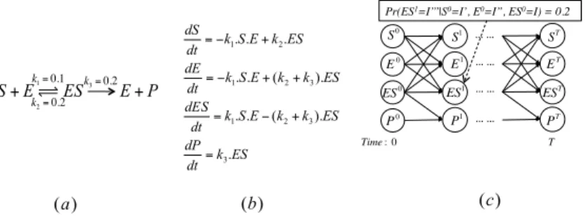
Liu et al. developed a dynamic Bayesian network approximation from a system of ODEs [16, 17] describing pathway dynamics to compactly store and analyze the dynamics of the original system. Its main features are illustrated by a simple enzyme kinetics system shown in Fig. 1. In the original work, aspects of parameter uncertainty were considered, however, for simplicity, we will not deal with them in this study as it is not the focus of discussion in this paper.
The dynamics of the system is assumed to be of interest only for discrete time points up to a maximal time point. Let us assume that they are denoted as {0, 1, . . . , T }.
There is random variable Yicorresponding to every molecular species yi. The range of
each variable Yi is quantized into a set of intervals Ii = {I0i, . . . , IK−1i }, with K the
number of intervals for variable Yi. The quantized dynamics is intrinsically stochastic,
as even for deterministic dynamics (e.g. of an ODE system), it is possible that two distinct deterministic configurations correspond to the same quantized configuration, but their deterministic successors are in distinct quantized configurations. Initial values of the system are assumed to follow a distribution. Initial configurations are sampled according to this distribution, and trajectories are generated by simulating the system
) (b (c) ES k dt dP ES k k E S k dt dES ES k k E S k dt dE ES k E S k dt dS . ). ( . . ). ( . . . . . 3 3 2 1 3 2 1 2 1 = + − = + + − = + − = ) (a ES E S + k1= 0.1 E +P k2= 0.2 k3= 0.2 dS dt= −0.1⋅ S ⋅ E + 0.2 ⋅ ES dE dt= −0.1⋅ S ⋅ E + (0.2 + r3)⋅ ES dES dt = 0.1⋅ S ⋅ E − (0.2 + r3)⋅ ES dP dt= r3⋅ ES !! !! …"…" …"…" …"…" …"…" € ST € EST € ET € PT € S1 € ES1 € E1 € P1 € S0 € ES0 € E0 € P0 €
Pr(ES1= I''| S0= I', E0= I, ES0= I'',r 3 0= I') = 0.4 € 0 € T € Time : € (c) € (b) ES E S + E +P € r1= 0.1 € r3 € r2= 0.2 € (a)
Pr(ES1=I’’’|S0=I’, E0=I’’, ES0=I) = 0.2
Fig. 1. a) The enzyme catalytic reaction network (b) The ODEs model (c) The DBN approxima-tion for 2 successive time points
from these samples. These trajectories are then compactly approximated as a DBN, treated as an approximation of the dynamics of the system.
For this, the reaction network is used to define the structure (local dependency
rela-tion). As discussed before, there is one random variable Yitfor each molecular species
yiat time t. The node Ybt−1will be in Pa(Y
t
i) iff b appears in the mathematical equation
of species yior if i = b.
CPT entries are of the form Cit(v | l) = p, which says that p is the probability of
the value of Yifalling in the interval Ivi at time t, given that for each Y
t−1
j ∈ P a(Y
t
i),
the value of Yjwas in I
j
lj . We evaluate this probability p through simple counting. For
instance, among the generated trajectories, the number of simulations where the value
of Yjfalls in the interval I
j
lj at time t − 1 simultaneously for each j ∈ ˆi is recorded, say
Jl. Next, among these Jltrajectories, the number of these where the value of Yifalls in
the interval Ii
vat time t is recorded. If this number is Jvthen the empirical probability
p is set to beJv
Jl. We refer interested readers to Liu et al.’s work [16] for the details.
We thus haveP
v∈V C
t
i(v | l) = 1. There is a special case when Jl= 0 where we
set p = 0. This implies thatP
v∈V Cit(v | l) = 0, since all these entries will be null.
In this case, we will say that the DBN has singularities. This happens when the tuple of intervals corresponding to l has not been visited at time point t − 1 by simulating the original system. This is actually the case for a majority of the entries of the DBNs generated from all the biological pathways we tested on (see Section 4 and experimental results in Table 1).
2.3 Singularities in DBNs
In this section, we will illustrate how a DBN is generated from a simple system with two variables. We will explain how singularities appear in DBN obtained in such a way, and potential problems arising from these singularities.
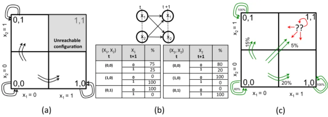
Consider a system with 2 variables X1and X2each of whom take values from the
discrete set {0, 1}. Figure 2 (a) shows the possible configurations of the system for all value assignments of the variables. For instance, the rectangle corresponding to (0, 0)
means that the system is at configuration defined by X1 = 0 and X2 = 0 and so on.
1,0 0,0 1,1 0,1 x2 = 1 x2 = 0 x1 = 0 x1 = 1 (a)$ (b)$ (X1,$X2)$$$ t" t+1"X1$$ %$ (0,0)" 0" 1" (1,0)" 0" 1" (0,1)" 0" 1" Unreachable"" configura6on" (c)$ 1,0 0,0 1,1 0,1 x2 = 1 x2 = 0 x1 = 0 x1 = 1 ??$ 60% 15% 20% 5% 100% 100% x1 x1 x2 x2 t t +1 (X1,$X2)$$$ t" t+1"X2$$ %$ (0,0)" 0" 1" (1,0)" 0" 1" (0,1)" 0" 1" 75$ 25$ 80$20$ 0$ 100$ 100$ 100$ 100$ 0$ 0$ 0$
Fig. 2. a) The dynamics defined by the 2 variable system (b) The assumed DBN model and the CPT entries (c) According to the DBN, every configuration is reachable, including (1, 1) from which no CPT entry is defined.
the configuration (1, 1) i.e., the system cannot reach the configuration with both X1= 1
and X2 = 1. More precisely, if the system is in configuration (0, 0) at time t, at time
t + 1, it can stay in the same configuration (0, 0), or go to configuration (0, 1) or (1, 0). However, it cannot go to configuration (1, 1).
Fig. 2 (b) shows the DBN construction from the system in Fig. 2 (a), as outlined in
the previous subsection. Variables X1t+1, X2t+1are dependent on both X1tand X2t, as
shown on the top part of the figure. The bottom part of Fig. 2 (b) shows the conditional
probability table for X1t+1and X2t+1. For instance, in the table for X1t+1, the first
col-umn describes the parent configuration tuples, i.e, the values for X1tand X2t. The second
column describes the value X1t+1can take. The third column represents the
correspond-ing probabilities. The first row describes that if (X1t, X2t) = (0, 0), then X
t+1
1 taking
value 0 (resp. 1) has probability 75% (resp. 25%) of happening. This CPT is stochastic: P v∈{0,1}C t i(v | (0, 0)) = P v∈{0,1}C t i(v | (0, 1)) = P v∈{0,1}C t i(v | (1, 0)) = 1.
Notice that owing to the system dynamics, there is no value in the CPT
correspond-ing to (Xt
1, X2t) taking value (1, 1), which is a source of singularity in the CPT. Two
problems arise from singularities, as shown in Fig. 2 (c). First, from configuration
(Xt
1, X2t) = (0, 0), there is a (small but non null) probability to sample 1 for
vari-able X1t+1and 1 for variable X2t+1, and thus to end up in configuration (1, 1). This is a
problem because configuration (1, 1) does not correspond to a behavior of the original system. An additional problem is that from this singular configuration (1, 1), there is no defined outgoing probability distribution.
3
Simulation Algorithms
In this section we will first discuss the usual simple algorithm for simulating DBNs. These simulations can potentially encounter singular configurations. In the simple al-gorithm, such simulations, called unsuccessful, are discarded since they may lead to inefficiencies and inaccuracies. We will propose two algorithms to circumvent this is-sue. The first algorithm simulates CPT entries which are singular by choosing successor configurations uniformly at random. It can be very efficient, although it can be more er-ror prone than simple simulations. Our main contribution is the design of the look-ahead simulation algorithm, which samples configurations of the DBNs in such a way to avoid singularities. It thus produces lower unsuccessful simulations, but could be slower.
3.1 Simple Simulation Algorithm
The simple simulation, as shown in Alg. 1, samples every variable independently. It
draws a value wifor each variable (the for loop at line 2) according to the distribution
described by Ct
i(. | vˆi) for v the value assignment which has been sampled at the
previous time point (recall that vˆi restricts v to the subset of parents of i). For t = 0,
wiis initialized according to the distribution P (Xi0). The for loop at line 10 checks if
the new configuration is singular, in which case the simulation is discarded (Abort at line 15). Such a simulation is termed unsuccessful. We consider for each variable i the
set P reti(line 11) of tuples l of values at time t over the set of parents ˆi of node i, and
which have been seen in the simulations (that isP
k∈KC
t
i(k | l) = 1).
For instance, with the DBN in Fig. 2 (b), from configuration (0, 0), there is a small
chance to sample w1 = 1 (e.g. x = rand([0, 1]) = 0.9 which will enter the while
loop once and set y at 1) and w2 = 1 (for the same reason), in which case the test
wˆ1= (1, 1) /∈ P re
t
i= {(0, 0), (1, 0), (0, 1)} (line 11) raises the exception Abort.
Algorithm 1 Simple Simulation of DBNs
1: for t = 0..T do 2: for i = 1, ..., n do 3: x ← rand([0, 1]) 4: y ← 0 5: z ← Ct i(y | vˆi) . % For t = 0, C 0 i(y | vˆi) = C 0 i(y) = P (Xi0) 6: while x > z do 7: y ← y + 1, z ← z + Ct i(y | vˆi) 8: wi← y 9: if t > 0 then 10: for i = 1, ..., n do 11: P reti← {l ∈ V ˆi|P k∈KC t
i(k | l) = 1} . Set of possible value assignments
for ˆi 12: if wˆi∈ P re t ithen 13: vi← wi 14: else 15: Abort
3.2 Uniform Simulation Algorithm
A naive solution to avoid unsuccessful simulations is to assume a predetermined CPT
entry Cit(y | vˆi) for singular cases where
P
y∈VC
t
i(y | vˆi) = 0. For simplicity and
compactness of the representation, we assume uniform probabilities: Cit(y | vˆi) = 1/K
(with K the number of values in V ) for all y ∈ V for singular vˆiat time t. In this case,
for every t, i and every vˆi, we have
P
y∈VC
t
i(y | vˆi) = 1.
The uniform stimulation algorithm thus uses the simple simulation of Fig. 1, how-ever with fully defined CPTs. As a result of this, we no longer have the issue of drawing unsuccessful samples. The for loop from line 10 to 15 is unnecessary and hence re-moved. Although this results in speed-up of drawing effective simulations (all samples are effective), the underlying dynamics can be less accurate, as the information that l has not been sampled is lost with this uniform simulation.
For instance, with the DBN in Fig. 2 (b), from configuration (0, 0), there is a small chance to draw configuration (1, 1) (same as with the simple simulation). Now, using the uniform algorithm, simulations from (1, 1) are not discarded, and instead the system can go to any configuration of {(0, 0), (1, 0), (0, 1), (1, 1)}, with a 25% of chance for each.
3.3 Look-ahead Simulation Algorithm
In this section we propose a more involved simulation, called look-ahead simulation. The main idea is to sample tuples of values v representing the configuration at time t, according to the configuration y at time t − 1 and the corresponding CPTs, but con-ditioned to the fact that v has been seen at time t at least once during the original simulations of the system. Computing exactly this conditional probability is however not possible in general as that would require to recompute on the fly the probability for each of the many possible tuples v.
Instead, for efficiency reasons, we over-approximate this set of configurations. We fill up iteratively a partial value assignment W remembering the values of variables which have been already set (W [i] = −1 if i has not yet been set). The i-th iteration, focused on the variable i, assigns values for parents of i, that is for variables in ˆi. For
this, we consider the set P reti(W ) which only retains value assignments vˆifor ˆi at time
t which have been seen in the simulations and which are consistent with W .
Notice that by (inductive) construction of vˆj, C
t
i(l[j] | vˆj) is well defined at line 8.
In order to justify Algorithm 2, we prove that it is equivalent to Algorithm 1 in an ideal case where Algorithm 1 is correct. In particular, in that case, the distribution does not depend upon the order in which variables are considered in Algorithm 2.
Theorem 1. In the case where there is no singular configurations, Algorithm 2
gener-ates the same distribution over configurationsW than Algorithm 1.
Proof (Sketch of.). The probability of choosing W for Algorithm 1 is the product
Q
jC
t
j(W [j] | vˆj). We show by induction on the number of variables that W is also
generated with this probability by Algorithm 2. If there are no variables, this is trivial.
Since there are no singular configurations, P ret
i(W ) = {l ∈ V
ˆi
| ∀m with W [m] 6= −1, l[m] = W [m]}. We will show the property is true for W restricted to variables
Algorithm 2 Look-ahead simulation of DBNs
1: W [1, ..., n] = {−1, ..., −1} . W [i] = −1 means that the value of variable i is not yet set 2: for i = 1, ..., n do 3: P ret i(W ) = {l ∈ V ˆ i|P k∈KC t i(k | l) = 1 ∧ ∀m with W [m] 6= −1, l[m] = W [m]} 4: s ← 0
5: for all l ∈ P reti(W ) do . Compute the probabilities for value assignments in P re t i(W )
6: p ← 1
7: for all j ∈ ˆi do . Compute probabilities of l 8: p ← p · Ct
i(l[j] | vˆj)
9: P rob[l] ← p
10: s ← s + p . Sum of probabilities in P reti(W )
11: if s = 0 then Abort . No configurations are consistent with W 12: x ← rand([0, s])
13: z ← 0
14: for all l ∈ P reti(W ) do . Pick a l according to P rob
15: z ← z + P rob[l]
16: if x ≥ z then . The current l has been chosen for variables in ˆi 17: for all j ∈ ˆi do
18: W [j] ← l[j] 19: break
20: for i = 1, ..., n do 21: vi← W [i]
is easy to see that at line 10 of Algorithm 2, s will be equal to s =Q
j∈JC
t
j(W [j] | vˆj),
because for all j ∈ ˆi \ J ,P
l[j]C
t
i(l[j] | vˆj) = 1 (no singular configurations). Hence
choosing W |I0 will be done with probability
Q j∈ˆiC
t
j(W [j]|vˆj)
s (to select Wˆi\J at line
14), times P rob(W |{j|W [j]6=−1}) (to have selected W |{j|W [j]6=−1}after i − 1). By
in-duction hypothesis, the second term isQ
j|W [j]6=−1C
t
j(W [j] | vˆj). The first term can
be simplified intoQ
j∈ˆi\JC
t
j(W [j] | vˆj)ss. This proves the result by induction.
The set of value assignments vˆi for ˆi which have been explored is small (< 1000,
see Table 1 in Section 5.1), compared to the set of visited value assignments v for all
variables. In order to set a value assignment vˆi for variables in ˆi, we draw one value
assignment in P ret
i(W ), according to its probability w.r.t. the sum of probabilities of
all value assignments in P ret
i(W ) (that is the probability of drawing a value assignment
in P ret
i(W ) is the same as for the simple simulation, but conditioned to the fact that a
value assignment of P ret
i(W ) is drawn). If all variables of W can be set in this way,
then by definition we have that W is not a singular configuration.
This look-ahead algorithm can however be quite slow because of the overhead of recomputing probabilities conditioned to sampling only non singular configurations. To speed up the process, we use an adaptive procedure, which first uses the simple simulation, and only at the time point when a singularity is encountered uses the look-ahead algorithm to compute a new value assignment at this time point.
Notice that it may still be the case that the look-ahead algorithm Abort (line 11), in
case where there is no value assignments in P ret
i(W ) (that is s = 0).
For instance, in the example from Section 2.3, P ret=1
1 (W ) = P ret=11 ({−1, −1}) =
{(0, 0), (1, 0) , (0, 1)}. Starting from configuration (0, 0) at time t = 0, we compute P rob[(0, 0)] = 60%, P rob[(0, 1)] = 15%, and P rob[(1, 0)] = 20%. We have s = 95%, and we sample (0, 0) with probability 60/95. Notice that (1, 1) will never be gen-erated. Assume that (0, 0) is drawn (e.g. x = rand([0, 1]) = 0.5). Now, W = {0, 0},
and we have P ret=1
2 ({0, 0}) = {(0, 0)}. It gives P rob[(0, 0)] = 60%, s = 60% and
thus (0, 0) is sampled with probability 60/60 = 1. On this simple example, there is no unsuccessful trajectory using the look-ahead simulation.
4
DBN models considered in the experiments
In this section, we will introduce the case-studies that we use to construct DBNs and test the different DBN simulation algorithms we discussed in the previous section.
4.1 Enzyme catalytic kinetics
The enzyme catalytic system is shown in Fig. 1. It describes a typical mass action based kinetics of the binding (ES) of enzyme (E) with substrate(S) and its subsequent catalysis to convert the substrate into product (P). The value space of each variable is divided into 5 equal intervals. The time scale of the system is 10 minutes which was divided into
100 time points. To fill up the conditional probability tables, 5 · 105 trajectories were
generated from the ODE model.
4.2 EGF-NGF pathway
The EGF-NGF pathway describes the behavior of PC12 cell to EGF or NGF stimulation [3]. The ODE model of this pathway is available in the BioModels database [20]. It consists of 32 differential equations (one for each molecular species). As before, the value domains of the 32 variables were divided into 5 equal intervals. The time horizon of each model was set at 10 minutes which was divided into 100 time points. To fill up
the conditional probability tables, 5 · 105trajectories were generated by simulating the
ODE model.
4.3 Apoptosis pathway
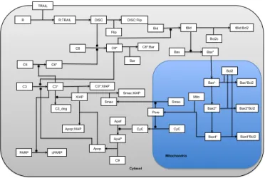
TNF-related apoptosis-inducing ligand (TRAIL) is a protein that is known to induce apoptosis in cancer cells and hence has been considered as a target for anti-cancer therapeutic strategies. However, biological observations suggest that in a population of cells, application of TRAIL leads to only fractional killing of cells (for instance, 70% of deaths after 8 hours for 250ng/ml of TRAIL) and also a time dependent evolu-tion of cell resistance to TRAIL. Several models have been proposed to understand this mechanism, specifically an Hybrid Stochastic Deterministic (HSD) model [1] which combines a deterministic signal transduction model (modeled as ordinary differential equations (ODEs)), and a stochastic model for protein synthesis fluctuations (factoring cell-to cell variability). The model consists of 58 protein variables, the time horizon of the model was studied over an 8 hour period which was divided into 45 time points. To
fill up the conditional probability tables, 5·105trajectories were generated by simulating
R TRAIL
R:TRAIL DISC DISC:Flip Bid Bcl2c tBid:Bcl2 Bax tBid C8*:Bar Bar Flip C8* Bax* C3*:XIAP XIAP C3_deg C3* C3 C6* C6 C8 Apop Smac Smac:XIAP Apop:XIAP cPARP PARP C9 Apaf* Apaf CyC CyC Pore Smac Bax* Bax2* Bax4* Bcl2 Bax*Bcl2 Bax2*Bcl2 Bax4*Bcl2 Mito Mitochondria Cytosol
Fig. 3. Apoptosis pathway
5
Experiments
We now evaluate the different DBN simulation algorithms on the DBNs generated for the systems described before. We measure the % of effective samples, mean error, and time taken per effective sample to assess the different approaches. We also discuss the aspect of sparsity in CPTs for all of these DBNs.
5.1 Sparse CPTs.
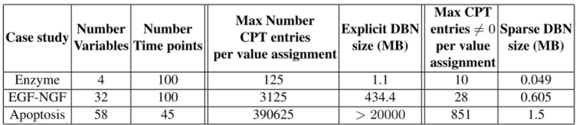
For each of the DBNs that we constructed, Table 1 shows the base statistics in terms of the number of variables and time-points considered for them. For a DBN, the maximal
number of CPT entries corresponding to any variable of the DBN is given by KN +1
where N the maximal number of parents any node of the DBN can have and K is the cardinality of that node. For instance, in the enzyme kinetics system, N = 3 (see Fig.1). Similarly, N = 5 for EGF-NGF pathway and N = 8 for apoptosis pathway. In all our case studies K = 5 for all variables, the number of discrete intervals we assume. If represented explicitly, these entries potentially make for a large CPT table, whose size is reported in MB. These numbers are shown in Table 1.
As explained in Section 2.3, some of these entries may be 0 since they have not been visited by system simulations used to build the DBN. Actually, we notice that most of
the entries are in fact null: only at most 10 (resp. 28 and 851) out of the KN +1entries are
non null (reported in the last but one column). This simple observation leads to a sparse representation for DBNs which is very compact (last column). All analysis on DBNs can be adapted to this sparse representation, which was not exploited in e.g. [16, 17].
Over all the systems we tested, ranging from very simple to more complex ones, we found that all of them exhibit very sparse CPTs. The main reason for this can be attributed to the fact that parents of nodes are usually very correlated and capture the underlying dynamics well, and while they can individually take all of the 5 values, only very few of the combinations are observed in the systems, which explain why the sparse representation is so efficient.
Case study Number Variables Number Time points Max Number CPT entries per value assignment
Explicit DBN size (MB) Max CPT entries 6= 0 per value assignment Sparse DBN size (MB) Enzyme 4 100 125 1.1 10 0.049 EGF-NGF 32 100 3125 434.4 28 0.605 Apoptosis 58 45 390625 > 20000 851 1.5 Table 1. Sparsity in CPTs
Notice that although CPT entries are sparse (because parents of nodes are highly correlated), it is not the case for the joint distributions over all the variables. For in-stance, in the apoptosis pathway, out of 200000 simulations, 95% of the simulations resulted in distinct joints, that is very few end up having the same joints (at most 5% reach the same joints). This implies that explicitly keeping every non null joints over all variables is not feasible, although it is a practical once restricted to parents of a variable (which is what the DBN encodes well with a sparse encoding).
5.2 Evaluation of simulation algorithms
We designed tests to compare the different simulation algorithms presented in Section 3 (called simple, uniform and adaptive (for the adaptive look-ahead algorithm) in the Ta-bles 2 and 3). We evaluated them on the different DBNs generated from the biological systems described in Section 4. For all case studies reported here we perform experi-ments by drawing 10000 samples from the underlying DBN and analyzing them.
We mainly measure and compare a) the % of effective runs for the algorithms (not reported for uniform simulation as it is always 100%), b) the time needed for each effective simulation, and c) the difference between outputs of these three algorithms and the original dynamics (Enzyme, EGF-NGF, Apoptosis), in terms of mean error of the different trajectories. Mean error is computed as mean over the weighted difference between the marginals computed by the DBN algorithm and marginals of the quantized traces of the original system of each variable
All results are summarized in Table 2. For the enzyme kinetics system, almost all simple simulations are effective (98%), and so all the three algorithms show no tangible difference, with a very good agreement with the dynamics of the original biological pathway.
Case study effectiveness simple | adaptive
time per effect. sample uniform | simple | adaptive
mean error
uniform | simple | adaptive Enzyme 98% | 100% 1.81ms | 2.33ms | 2.26ms 0.454% | 0.347% | 0.429% EGF-NGF 36% | 100% 20.3ms | 30.4ms | 26.8ms 2.22% | 1.63% | 1.30% Apoptosis 3.1% | 83% 8.46 ms | 121 ms | 68.0ms 14.7% | 6.82% | 4.47%
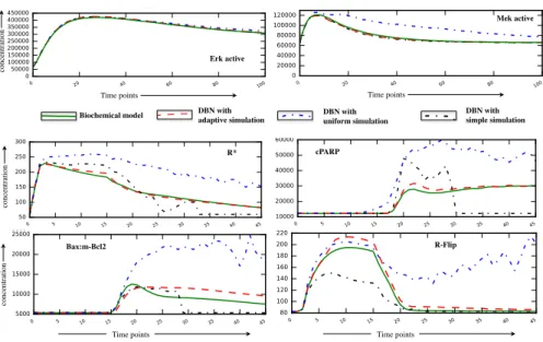
conc ent ra ti on Time points Mek active Erk active R* cPARP R-Flip Bax:m-Bcl2 Time points
Biochemical model DBN with!adaptive simulation DBN with! uniform simulation DBN with! simple simulation Time points conc ent ra ti on conc ent ra ti on Time points conc ent ra ti on Time points Mek active Erk active R* cPARP R-Flip Bax:m-Bcl2 Time points
Biochemical model DBN with!adaptive simulation DBN with! uniform simulation DBN with! simple simulation Time points conc ent ra ti on conc ent ra ti on Time points
Fig. 4. Mean value of trajectories for selected species in the EGF-NGF pathway (top 2) and in the apoptosis pathway (bottom 4), as simulated by the biochemical model (solid green), the DBN using the simple simulations (black), adaptive look-ahead simulations (red), and uniform simulations (blue).
For the EGF-NGF case, there was a clear percentage of unsuccessful simple simu-lations (64%), and the three algorithms give considerably different results. The adaptive look-ahead algorithm is overall more faithful than the simple simulation while being as fast, however, the uniform algorithm is faster but less accurate (70% more errors than the adaptive look-ahead algorithm). The mean error may seem small because for most proteins, there is a very low error (e.g. ERK active in Fig. 4 top left), although tangible difference could be seen (especially using the uniform simulation) on few proteins (e.g. Mek active in Fig. 4 top right).
For Apoptosis, the number of effective simple simulations was very low (3.1%), and the errors of our algorithms w.r.t. the biological system were larger, as shown in Fig. 4 (bottom). The simple algorithm was the slowest and quite inaccurate, due to very few effective samples. The uniform algorithm was very fast, while being very inaccurate, with very large errors on some proteins, as shown in Fig. 4 (bottom).
Overall, the adaptive look-ahead algorithm succeeds in bringing up to 24 times (Apoptosis in Table 2) more effective samples compared with the simple simulation. It fails to reach 100% only in the extreme case where most simple simulations fail. The adaptive look-ahead simulation clearly improves the accuracy of the simulation. Last, runtime is not impacted by choosing adaptive look-ahead over simple simulation. Instead, in extreme case, adaptive look-ahead simulation can outperform simple simu-lations in the number of effective samples being simulated per unit of time (Table 2).
There might be specific cases where the performance of simulation algorithms can become very important, for instance, when the simulations can have different lengths
apoptosis HSD model Uniform simulation Simple simulation Adaptive simulation dead cells 70% 99.4% 99.7% 73% Table 3. percentage dead cells for different simulation strategies
(e.g. a simulation is truncated when a cell dies in the apoptosis pathway). In this case, a DBN simulation can lead to configurations of the system representing cell death. If the simulation reached some of these configurations, then the cell is declared dead and no further simulation is performed. This also means that an alive cell will have simulation traces equal to the number of time points considered. Consequentially, owing to the limitations of the simple simulation, generating alive cells is considerably harder. This is evident in Table 3, where the simple and uniform strategy produce > 99% cell death, while the original system dynamics [1] predicts a 70% death rate.
The simple strategy also has an extremely low efficiency (3.1%): almost all effective simple simulations of the apoptosis pathway end up dead (99.7%). Uniform simulations give very inaccurate results as well (99.4% vs 70% of dead cells). On the other hand, using the look-ahead simulation, most of the simulations are effective (83%). We also obtain a death rate close to the one of HSD model (73% instead of 70%).
6
Conclusions
In this paper, we have highlighted and systematically characterized singularities ob-served in DBNs obtained as abstractions of biological pathway dynamics [17] follow-ing the method of [16]. The main characteristic of these DBNs is that many entries of the CPTs are null. We show that this can be used to vastly improve the representation of DBNs using sparse encoding. However, it is also a source of inaccuracy when simulat-ing these DBNs. Compared with the usual algorithm which is used to simulate DBNs, we propose two different simulation algorithms. First, a uniform simulation procedure which is faster but also less accurate. This should be preferred when time as a resource is limited and a crude evaluation is sufficient. More importantly, we developed a new adaptive look-ahead simulation which is comparable in run time or faster than simple simulation and also is the most accurate, as it produces very limited number of unsuc-cessful simulations compared to simple simulations (up to 24 times less). In terms of future work, we plan to develop a class of models more accurate than DBNs, that would encode probabilities of tuples of variables in CPTs rather than over single variables.
Acknowledgments
This work was partially supported by ANR projects STOCH-MC (ANR-13-BS02-0011-01) and Iceberg (ANR-IABI-3096).
References
1. F. Bertaux, S. Stoma, D. Drasdo, and G. Batt. Modeling Dynamics of Cell-to-Cell Vari-ability in TRAIL-Induced Apoptosis Explains Fractional Killing and Predicts Reversible Resistance. PLoS Computational Biology, 10(10):14, 2014.
2. X. Boyen and D. Koller. Tractable inference for complex stochastic processes. In UAI-98, pages 33–42, 1998.
3. K. S. Brown, C. C. Hill, G. A. Calero, K. H. Lee, J. P. Sethna, and R. A. Cerione. The statistical mechanics of complex signaling networks: nerve growth factor signaling. Physical Biology 1, pages 184–195, 2004.
4. M. Calder, V. Vyshemirsky, D. Gilbert, and R.J. Orton. Analysis of signalling pathways using continuous time markov chains. T. Comp. Sys. Biology, pages 44–67, 2006.
5. V. Danos, J. Feret, W. Fontana, R. Harmer, and J. Krivine. Rule-based modelling of cellular signalling. In CONCUR, pages 17–41, 2007.
6. F. Didier, T. A. Henzinger, M. Mateescu, and V. Wolf. Approximation of event probabilities in noisy cellular processes. Theor. Comput. Sci., 412, 2011.
7. R. Donaldson and D. Gilbert. A model checking approach to the parameter estimation of biochemical pathways. In CMSB, pages 269–287, 2008.
8. F. Fages and A. Rizk. On the analysis of numerical data time series in temporal logic. In CMSB’07, LNCS 4695, pages 48–63, 2007.
9. R. Grosu and S. A. Smolka. Monte carlo model checking. In TACAS, pages 271–286, 2005. 10. T.A. Henzinger, M. Mateescu, and V. Wolf. Sliding window abstraction for infinite markov
chains. In CAV, pages 337–352, 2009.
11. S. K. Jha, E. M. Clarke, C. J. Langmead, A. Legay, A. Platzer, and P. Zuliani. A bayesian approach to model checking biological systems. In CMSB, pages 218–234, 2009.
12. D. Koller and N. Friedman. Probabilistic Graphical Models - Principles and Techniques. MIT Press, 2009.
13. M. Z. Kwiatkowska, G. Norman, and D. Parker. Symbolic Systems Biology, chapter Proba-bilistic Model Checking for Systems Biology. Jones and Bartlett, 2010.
14. M.Z. Kwiatkowska, G. Norman, and D. Parker. PRISM: Probabilistic symbolic model checker. In TOOLS’02, LNCS 2324, pages 200–204, 2002.
15. B. Liu, A. Hagiescu, S. K. Palaniappan, B. Chattopadhyay, Z. Cui, W.-F. Wong, and PS Thi-agarajan. Approximate probabilistic analysis of biopathway dynamics. Bioinformatics, 28(11):1508–1516, 2012.
16. B. Liu, D. Hsu, and P.S. Thiagarajan. Probabilistic approximations of ODEs based bio-pathway dynamics. Theor. Comput. Sci., 412:2188–2206, May 2011.
17. B. Liu, P. S. Thiagarajan, and D. Hsu. Probabilistic approximations of signaling pathway dynamics. In CMSB, LNCS 5688, Springer, pages 251–265, 2009.
18. B. Liu, J. Zhang, P.Y. Tan, D. Hsu, A. Blom M., B. Leong, S. Sethil, B. Ho, J.L. Ding, and P.S. Thiagarajan. A computational and experimental study of the regulatory mechanisms of the complement system. PLoS Comput Biol, 7(1):e1001059, 01 2011.
19. K.P. Murphy and Y. Weiss. The factored frontier algorithm for approximate inference in DBNs. In UAI’01, pages 378–385, 2001.
20. N. Le Novere, B. Bornstein, A. Broicher, M. Courtot, M. Donizelli, H. Dharuri, H. Sauro L. Li, M. Schilstra, B. Shapiro, J. Snoep, and M. Hucka. Biomodels database: A free, central-ized database of curated, published, quantitative kinetic models of biochemical and cellular systems. Nucleic Acids Research 34, pages D689– D691, 2006.
21. S. K. Palaniappan, S. Akshay, B. Genest, and P. S. Thiagarajan. A hybrid factored frontier algorithm. TCBB, 9(5):1352–1365, 2012.
22. W.S.Hlavacek, J.R.Faeder, M.L.Blinov, R.G.Posner, M.Hucka, and W.Fontana. Rules for modeling signal-transduction systems. Science STKE, 2006:re6, 2006.