Box consistency through Adaptive Shaving

HAL Id: hal-00428678

https://hal.archives-ouvertes.fr/hal-00428678

Submitted on 29 Oct 2009

HAL is a multi-disciplinary open access

archive for the deposit and dissemination of

sci-entific research documents, whether they are

pub-lished or not. The documents may come from

teaching and research institutions in France or

abroad, or from public or private research centers.

L’archive ouverte pluridisciplinaire HAL, est

destinée au dépôt et à la diffusion de documents

scientifiques de niveau recherche, publiés ou non,

émanant des établissements d’enseignement et de

recherche français ou étrangers, des laboratoires

publics ou privés.

Box consistency through Adaptive Shaving

Alexandre Goldsztejn, Frédéric Goualard

To cite this version:

Alexandre Goldsztejn, Frédéric Goualard. Box consistency through Adaptive Shaving. 25th

Sympo-sium On Applied Computing, Mar 2010, Sierre, Switzerland. pp.2049-2054. �hal-00428678�

Box Consistency through Adaptive Shaving

Alexandre Goldsztejn

CNRS, LINA, UMR 6241 2 rue de la Houssini `ere BP 92208, F-44000 NANTES

Alexandre.Goldsztejn@univ-nantes.fr

Fr ´ed ´eric Goualard

Universit ´e de Nantes Nantes Atlantique Universit ´e

CNRS, LINA, UMR 6241 2 rue de la Houssini `ere BP 92208, F-44000 NANTES

Frederic.Goualard@univ-nantes.fr

ABSTRACT

The canonical algorithm to enforce box consistency over a constraint relies on a dichotomic process to isolate the left-most and rightleft-most solutions. We identify some weaknesses of the standard implementations of this approach and review the existing body of work to tackle them; we then present an adaptive shaving process to achieve box consistency by tightening a domain from both bounds inward. Experimen-tal results show a significant improvement over existing ap-proaches in terms of robustness for difficult problems.

Categories and Subject Descriptors

G.1.0 [Numerical

Analysis]: General—interval arithmetic

General Terms

Algorithms, Performance

Keywords

Local consistency, constraint programming, Newton method

1.

INTRODUCTION

Box consistency [1] is a local consistency notion for con-tinuous constraints. Stronger consistencies such as bounds consistency build on box consistency to achieve better do-main narrowing, which makes it pivotal in solving difficult constraint systems. Box consistency is usually enforced on unary projections of constraints by a combination of binary search and interval Newton steps to isolate leftmost and rightmost “quasi-zeroes” in the domain of a variable.

The canonical algorithm to enforce box consistency, de-scribed in details by Van Hentenryck et al. [6], is quite ro-bust and efficient on many problems. However, as we will see in Section 2, it is an intrinsically optimistic algorithm that always attempts to reduce large subdomains first during the dichotomic process without taking into account information

Permission to make digital or hard copies of all or part of this work for personal or classroom use is granted without fee provided that copies are not made or distributed for profit or commercial advantage and that copies bear this notice and the full citation on the first page. To copy otherwise, to republish, to post on servers or to redistribute to lists, requires prior specific permission and/or a fee.

SAC’10_{March 22-26, 2010, Sierre, Switzerland.} Copyright 2010 ACM 978-1-60558-638-0/10/03 ...✩5.00.

on the successes of its previous attempts. As experimental evidences presented in Section 4 show, this behavior makes it a largely suboptimal algorithm for many problems.

Early on, McAllester et al. [4] proposed a different view of the original algorithm to enforce box consistency in which it is no longer described as a recursive dichotomic process but as some kind of shaving process where a strict enforce-ment of box consistency is no longer the ultimate goal. In practice, this approach works well, except for those difficult problems for which it pays off to spend more time narrowing domains further in the contracting operator and defer less to the binary search process of the solver.

Following this track, we present in Section 3 an algorithm that enforces box consistency by an adaptive shaving pro-cess that takes into account past difficulties encountered in narrowing a domain down. Experimental evidences reported in Section 4 show that our new algorithm has more regular performances than McAllester et al.’s algorithm, even more so for difficult problems, where the later may flounder.

2.

BOX CONSISTENCY

Interval Constraint Programming makes cooperate con-tracting operators to prune the domains of variables (inter-vals with floating-point bounds from the set I) with smart propagation algorithms to ensure consistency among all the constraints. Exploration algorithms recursively split domains until a desired precision is achieved.

The amount of pruning obtained from one constraint is controlled by the level of consistency enforced. Box consis-tency considers interval extensions of the constraints. It is therefore parameterized by the interval extension used. In this paper, we only consider the natural interval extension of constraints, though our approach is not limited in any way to it. The same holds for the kind of constraints considered: while we limit ourselves to equations for the sake of simplic-ity, box consistency—and the algorithms presented—may be applied to inequations as well.

With these restrictions in mind, the definition of box con-sistency is as follows (using the notations for interval arith-metic advocated by Kearfott et al. [3], where interval quan-tities are boldfaced):

Definition 1 (Box consistency). The constraint f (x1, . . . ,

xn) = 0 is box consistent with respect to a variable xi and

a box of domains B = I1× · · · × In if and only if:

8 < : 0 ∈ f (I1, . . . , Ii−1, [Ii, Ii+], Ii+1, . . . , In) and 0 ∈ f (I1, . . . , Ii−1, [Ii−, Ii], Ii+1, . . . , In), (1)

Algorithm 1 Computing a box consistent interval [bc3revise(lnar,rnar )] in: g : I → I; in: I ∈ I

# Returns the largest interval included in I that is # box consistent with respect to g. The algorithm is # parameterized by the “lnar ” and “rnar ” methods used. begin

1 if0 /∈ g(I):

2 return ∅

3 return lnar(g, rnar(g, I)) end

where Ik= [Ik, Ik] are intervals with floating-point bounds,

a+ _{(resp., a}−_{) is the smallest floating-point number greater}

than (resp., the largest floating-point number smaller than) the floating-point number a, and f is the natural interval extension of f .

A constraint f (x1, . . . , xn) = 0 is box consistent with

re-spect to B if it is box consistent with rere-spect to x1, . . . , xn

and B. A constraint system is box consistent if all con-straints are box consistent.

In order not to lose any potential solution, an algorithm that enforces box consistency of a constraint with respect to a variable xi and a box of domains must return the largest

domain I′

i⊆ Ii that verifies Eq. (1).

Given a real function f : Rn

→ R and a box of domains B = I1× · · · × In ∈ In, we are hereafter only concerned

with interval projections g : I → I of f with respect to B, of the form:

g(x) = f (I1, . . . , Ii−1, x, Ii+1, . . . , In), i ∈ {1, . . . n}.

Algorithm bc3revise, presented by Alg. 1, enforces box consistency by searching the leftmost and rightmost canon-ical domains1 in the domain I of x for which g evaluates to an interval containing 0. It is parameterized by the two procedures lnar and rnar that perform the search for the left and right bounds respectively.

Algorithm bc3revise first tries to move the right bound of I to the left, and then proceeds to move its left bound to the right (this order could be reversed with no impact on performances, though).

In the original algorithm [1, 6], the search within lnar and rnaris performed by a dichotomic search aided with Newton steps to accelerate the process. Algorithm 2 describes the search of a quasi-zero to update the left side of I. The procedure rnarvhmakto update the right bound works along

the same lines and is, therefore, omitted.

The Newton procedure in Alg. 2 computes a step of the Interval Newton algorithm, that is, at iteration j + 1:

I(j +1)← I(j )∩ „ κ(I(j )) −g(κ(I (j )₎₎ g′_(I(j )₎ « (2) with κ(I) being a floating point number in I. The notation Newton(⋆) denotes the computation of Newton steps until reaching a fixpoint; we also use later the notation Newton(k) to denote an unspecified number of Newton steps (deter-mined by the context). The “hull ” notation ✷ (S) denotes the smallest interval (in the sense of set inclusion) contain-ing the set S; the notation m(I) denotes the midpoint of the interval I.

1_{A non-empty interval [a, b] is canonical if a}+_>b.

Algorithm 2 Computing a box consistent left bound [lnarvhmak] in: g : I → I; in: I ∈ I

# Returns an interval included in I

# with the smallest left bound l such that 0 ∈ g([l, l+]) begin

1 r ← I# Preserving the right bound

2 if0 /∈ g(I) : # No solution in I

3 return ∅

4 I← Newton(⋆)_{(g, g}′_{, I)# Interval Newton steps}

5 if I= ∅:

6 return ∅

7 if0 ∈ g([I, I+]): # Left bound is box consistent?

8 return[I, r]

9 else:

10 (I1, I2) ← split(I)# I1← [I, m(I)], I2← [m(I), I]

11 I← lnarvhmak(g, I1)

12 if I= ∅:

13 return ✷`lnarvhmak(g, I2) ∪ {r}´

14 else:

15 return ✷`I ∪ {r}´ end

Geometrically, an Interval Newton step reduces a domain I for an interval function g by computing the intersection between the x-axis and the area that contains all the lines passing through points in the segment (κ(I), g(κ(I)))−(κ(I), g(κ(I))) with slopes ranging in g′_{(I) (see Fig. 1 for an}

il-lustration). By the Mean Value Theorem, this area always encloses the graph of g on I, and thence its intersection with the x-axis contains all the solutions.

The Newton step expression (2) uses an extended ver-sion of the diviver-sion (hereafter noted “⊘”) to return a union of two open-ended intervals whenever g′_(I(j )_{) contains 0.}

The subtraction and the intersection operators are modi-fied accordingly: The intersection operator is applied to an interval (I(j )_{) and a union of two intervals (result of the}

subtraction), and returns an interval.

The lnarvhmakand rnarvhmak methods of the original

al-gorithm use the midpoint m(I(j )_{) of I}(j ) _{for κ(I}(j )_).

Ben-hamou et al. [1] considered using the left bound for lnar and the right bound for rnar but found that it could lead to slow convergence phenomena. On the other hand, as noted by McAllester et al. [4], a Newton expansion on a bound always yields some reduction of the domain.

For example, Fig. 2(a) presents a situation where the New-ton method cannot tighten a domain when expanding on the center of the domain (green area), while expanding on the left bound allows to tighten the domain on the left signifi-cantly (red area). However, Fig. 2(b) shows that this ability to always achieve some reduction may be more a curse than a blessing for problems where the derivative varies widely on the domain considered: no reduction occurs on the origi-nal domain [−8, 10], leading to splitting it and investigating separately the left part [−8, 1] (red line below the x-axis); from there, each step of the Newton method with an expan-sion on the left bound is able to shave the domain ever so slightly, leading to a very slow convergence (the reductions due to Newton steps are shown by the dashed lines below the x-axis). On the other hand, expanding on the center of the domain exhibits a different, more efficient behavior: no reduction occurs on the original domain, as in the pre-vious case; the left half sub-domain [−8, 1] (lowest red line above the x-axis) is investigated; no reduction occurs

be-−1.8 −1.6 −1.4 −1.2 −1 −0.8 −0.6 −0.4 −0.2 x −5.5 −4 −2.5 −1 0.5 2 y Original domain I Reduced domain g(x) g(x) “ κ(I), g(κ(I))” “ κ(I), g(κ(I))”

y = g′_{(I)(x − κ(I)) + g(κ(I))} y = g′_{(I)(x − κ(I)) + g(κ(I))} y = g′_{(I)(x − κ(I)) + g(κ(I))}

y = g′_{(I)(x − κ(I)) + g(κ(I))}

Figure 1: Interval Newton step with I = [−1.55, −1.2] and κ(I) = m(I)

cause the smallest and largest slopes corresponding to the derivative of the function on [−8, 1] are so steep that only a small portion in the middle of [−8, 1] could be removed; since we restrict ourselves to intervals, the whole domain is kept unchanged. The algorithm then splits the domain and considers [−8, −3.5], which can be discarded immediately by a simple evaluation of the function on it; the right part [−3.5, 1] is then considered, and so on. Note that, on this example, the algorithm with an expansion on the center ex-hibits a quite inefficient behavior of its own in that Newton steps are performed but can never achieve any reduction due to the steepness of the slopes on the [0, 1] subdomain.

3.

BOX CONSISTENCY BY SHAVING

McAllester et al. [4] consider the enforcement of box con-sistency as a shaving process where the bounds of a domain are moved inward by trying to discard “slices” of varying sizes on the left and right of the domain. The result is an algorithm whose most natural presentation is no longer re-cursive (cf. Alg. 2). We present in Alg. 3 a generic shaving algorithm for the left bound that uses the interval Newton operator2. The slice to be processed is defined by choosing a value p (Line 4). The reduction process is then applied to the slice guess = [I, p].

To shave a domain [a, b] on, say, the left side, we must choose a slice [a, p] ⊆ [a, b] that we will try to discard, and a value for κ([a, p]). The larger [a, p] the better, provided we are able to discard it. On the other hand, a large [a, p]

2_{Note, however, that McAllester et al.’s algorithm}

slightly differs from Alg. 3 in that their purpose is only to move the left and right bounds inward by a “reasonable” amount (in their paper, they consider that reducing a do-main by 10% or more is a reasonable goal to achieve for a contracting operator), which means that they may not en-force box consistency.

−24 −18 −12 −6 0 6 12 18 24

x

y

Newton linearization at center

Newton linearization at left bound Extreme slopes on [−25, 25]

(a) Expansion on bound vs. expansion on center

−6 −4 −2 0 2 4 6 8

x

y

Expansion in the middle

Expansion on the left bound

(b) Slow convergence

Figure 2: Box consistency enforcement. Interval functions have magenta borders and a light blue sur-face. In Figure 2(b), red domains are obtained by dichotomy; blue domains are discarded by an eval-uation of the function; green domains are narrowed by a Newton step.

−8 −6 −4 −2 0 2 4 6 8 10

x

y

(a) Expansion on center

−8 −6 −4 −2 0 2 4 6 8 10

x

y

(b) Expansion on left bound

Figure 3: Shaving process for the left side. Ini-tial domain is [−8, 10]; Slices considered are [−8, −3.5] (dark red area) and [−8, 0] (light red area).

Algorithm 3 Enforcing box consistency by shaving [lnarshaving] in: g : I → I; in: I ∈ I

begin

1 # Non-empty I is not box consistent on left?

2 while I6= ∅ ∧ 0 /∈ g([I, I+_]):

3 I← [I+_{, I]# We already know 0 /∈ [I, I}+_]

4 p ←choose a floating-point in I

5 guess ← [I, p]

6 if0 /∈ g(guess):

7 reduced ← ∅

8 else:

9 # Performing one or more Newton steps

10 # (determined by the instantiation of the alg.)

11 reduced ← Newton(k)(g, g′_{, guess)}

12 # Keep the right bound unchanged:

13 I← ✷`reduced ∪ (I \ guess)´

14 return I end

often entails a large domain for the derivative on [a, p], which leads to less shaving. The same problem holds for the choice of κ([a, p]): taking κ([a, p]) = a ensures that we will shave the left part of [a, b], however slightly. Values farther from a potentially offer better cuts, while they may also lead to no reduction at all.

All these situations are presented in Figures 3(a) and 3(b): Given the initial domain [−8, 10], choosing a small slice, such as [−8, −3.5], is often a sufire way of achieving some re-duction, which may be large compared to the size of the slice, though it is proportionally small compared to the initial do-main. Here, we obtain approximately [−3.68, −3.5] for the expansion point on the center (dark red cone in Fig. 3(a)), and [−4, −3.5] for an expansion on the left bound (dark red cone in Fig. 3(b)). For this problem, choosing a small slice leads to a large reduction (relatively to the size of the slice) for both expansion points. For some “well-behaved” functions, however, larger slices have the potential of larger reductions. The same dilemma arises in choosing the expan-sion point: Comparing Fig. 3(a) and Fig. 3(b), we see that for the slice [−8, −3.5], an expansion point on the center of-fers a better reduction than on the left bound; The reverse is true for the slice [−8, 0] (light red cones in Fig. 3(a) and Fig. 3(b)), where an expansion on the center leads to no re-duction at all because the part to discard is strictly included in the domain considered. On the other hand, the expan-sion on the left bound always leads to some reduction, as promised above.

To shave the left part of a domain [a, b], the algorithm presented by McAllester et al. [4] first considers the slice formed by the whole domain. If the reduction obtained by a Newton step does not lead to a reduction by 10% or more, it considers the left half [a, (a + b)/2]; again, if the reduction is insufficient, it considers the leftmost quarter of the initial domain, [a, (3a+b)/4]. Lastly, if the reduction is still insuffi-cient, it considers the leftmost eighth, [a, (7a+b)/8]. At that point, it returns whatever domain [l, b] was obtained, even if its left bound is not box consistent (i.e. 0 6∈ g([l, l+_{])). For}

all Newton steps performed, it uses the center of the domain under scrutiny as the expansion point, in a bid to achieve large reductions.

Following McAllester et al.’s work, we have designed an algorithm that uses a different shaving process to address its shortcomings (see discussion below). The corresponding left narrowing procedure lnarsbc3ag is presented in Alg. 4

(The rnarsbc3ag procedure is not shown, since it can easily

be obtained from lnarsbc3ag by symmetry). An important

difference with McAllester et al.’s algorithm is that ours en-forces box consistency every time, while theirs usually stops the narrowing process before that point. As Section 4 will show, spending more time to effectually enforce box con-sistency is the key to good performances for some difficult problems.

To shave the left part of a domain [a, b], we proceed as follows (see Alg. 4): We consider a slice whose width is γ times the width W of the initial domain, and we apply one Newton step on it; if the reduction obtained is smaller than some threshold σb, we update γ to βbγ, with βb< 1; if the

reduction is greater than some threshold σg, we update γ

to βgγ, with βg > 1. Otherwise, we keep γ as it is. We

then consider the next slice with a size equal to the new γ times W . In short, when we are able to shave large parts, we take larger bids; on the other hand, we decrease the size of the slices considered when things go wrong. This method follows the line of well-known numerical algorithms such as Trust Region Methods.

As shown in Alg. 4, the amount of reduction is computed by comparing the size of the previous domain with the size of the tightened domain where the right bound has been reset to the one of the previous domain (that is, we do not con-sider the possible displacement of the right bound as a useful reduction since it is not taken advantage of afterwards).

Another difference with McAllester et al.’s algorithm is that we use the left bound as an expansion point when shav-ing the left side (and the right bound when shavshav-ing the right side). There are two reasons for this: Firstly, this is a sure-fire strategy since it always lead to some reduction, as said previously; Secondly, we have to compute g([I, I+]) (Lines 3 and 20 in Alg. 4) before each Newton step to check whether the left bound is already box consistent. This value can be reused instead of g([I, I]) in the computation of the New-ton step Line 11 at a negligible cost in terms of the width of intervals involved (the correction of the process is obvi-ously preserved since we use a wider interval), while avoiding the cost of one function evaluation. Unreported experimen-tal evidences show that speed-ups up to 30% are attainable that way.

For the problem presented in Fig. 3, the original bc3revise algorithm [6] (that is, the one instantiated with lnarvhmak

and rnarvhmak) obtains the largest box consistent domain

(approximately [−0.487, 10]) after 50 Newton steps; McAlles-ter et al.’s algorithm stops with the non box consistent do-main [−3.5, 10] after only 6 Newton steps, and our algorithm enforces box consistency after 27 Newton steps.

4.

EXPERIMENTS

To evaluate the impact of our algorithm, we have selected 16 instances of 14 classical test problems. Some are poly-nomial and others are not. The characteristics of these test problems are summarized in Table 1. All problems are structurally well constrained, with as many equations as variables. Column “Constraints” indicates whether all con-straints are polynomial (quadratic, if no polynomial has a degree greater than 2). A problem is labelled “non-polyno-mial” if at least one constraint contains a trigonometric, hyperbolic or otherwise transcendental operator. Column “Source” gives a (not necessarily primary) reference to the literature where the problem is presented. The size of the

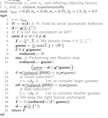
Algorithm 4 Enforcing box consistency on the left bound with adaptive guesses

[lnarsbc3ag] in: g : I → I; in: I ∈ I

# Thresholds σg and σb, and inflating/reducing factors

# βg and βbchosen experimentally.

const:γinit= 0.25, σg= 0.25, σb= 0.75, βg= 1.5, βb= 0.7

begin

1 γ ← γinit

2 W ← w(I)# W fixed to avoid asymptotic behavior

3 d← g([I, I+_])

4 # I is not box consistent on left? 5 while I6= ∅ ∧ 0 /∈ d:

6 I← [I+, I]# We already know 0 /∈ [I, I+_]

7 guess ← [I, min(I, I + γW )]

8 if0 /∈ g(guess)

9 reduced ← ∅

10 else:# Performing one Newton step

11 reduced ← guess∩

“

guess − d ⊘ g′_(guess)”

12 if w([reduced, guess]) < σgw(guess):

13 # Good reduction?. . .

14 γ ← γβg# . . . Let us consider larger guesses

15 elif w([reduced, guess]) > σbw(guess):

16 # Bad reduction?. . .

17 γ ← γβb# . . . Let us consider smaller guesses

18 # We keep the right bound unchanged:

19 I← ✷`reduced ∪ (I \ guess)´

20 d← g([I, I+_])

21 return I end

problem and the initial domains for the variables are given in Table 2.

Table 1: Test problems

Name Code Constraints Source

Broyden-banded bb quad. [6]

Broyden tridiagonal bt quad. [5]

Combustion comb poly. [6]

DBVF dbvf poly. [5]

Extended Freudenstein ef poly. COPRIN3

Extended Powell ep poly COPRIN3

Feigenbaum fe quad [2]

i4 i4 poly. [6]

Mixed Algebraic Trig. mat non-poly. COPRIN3

Mor´e-Cosnard mc poly. [6]

Trigexp te non-poly. COPRIN3

Trigexp 3 te3 non-poly. COPRIN3

Troesch tro non-poly. COPRIN3

Yamamura yam poly. COPRIN3

All experiments were conducted on an Intel Core2 Duo T5600 1.83GHz. The Whetstone test for this machine re-ports 1111 MIPS with a loop count equal to 100, 000.

All algorithms have been implemented in our own C++ constraint solver, with the not-yet-released version 4.0 of gaol4as the underlying interval arithmetic library.

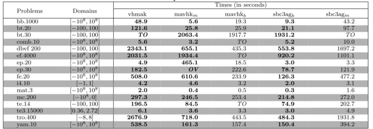
Table 2 reports the time spent in seconds to isolate all so-lutions of the test problems in domains with a width smaller than 10−8_{, starting from the initial domains given in}

Col-umn “Domains”. The number preceded by a dot in ColCol-umn “Problems” gives the number of equations and variables of the problem. An entry “TO” indicates a time-out (fixed to more than one hour, here). An entry “OV” indicates

3_{http://www-sop.inria.fr/coprin/logiciels/ALIAS/}

Benches/benches.html

Table 2: Experimental Results

Times (in seconds)

Problems Domains

vhmak mavhkm mavhkb sbc3agb sbc3agm

bb.1000 [−108_{, 10}8_{] 48.9 5.6 19.3 9.3 43.2} bt.20 [−100, 100] 121.6 25.8 25.9 21.1 97.7 bt.30 [−100, 100] TO 2063.4 1917.7 1931.2 TO comb.10 [−108_{, 10}8_{] 5.6 3.2 TO 5.2 10.0} dbvf 200 [−100, 100] 2343.1 655.1 435.3 553.8 1697.2 ef.4000 [−108_{, 10}8_{] 2031.5 1934.4} TO _{920.2 1101.1} ep.20 [−108_{, 10}8_{] 4.9 465.1 18.5 3.0 3.3} ep.30 [−108_{, 10}8_{] 182.5} OV _{222.6 78.7 121.9} fe.20 [−108_{, 10}8_{] 508.0 610.6 233.9 126.3 477.2} i4.10 [−1, 1] 4.2 4.6 3.2 2.0 3.1 mat.3 [−108_{, 10}8_{] 2.0 0.4 0.5 0.3 1.6} mc.200 [−108_{, 0] 297.3 246.5 253.4 214.8 272.0} te.14 [−100, 100] 196.5 84.5 TO _{74.9 202.7} te3.15000 [0.36, 2.72] 6.1 3.6 3.3 3.0 4.9 tro.400 [−8, 8] 2676.9 718.0 443.5 484.3 1931.8 yam.10 [−108_{, 10}8_{] 538.5 161.3 157.4 150.4 394.2}

Times on an Intel Core2 Duo T5600 1.83GHz (whetstone 100 000: 1111 MIPS). Time-out set to 1 hour.

that an overflow (stack or heap) prevented the computation to complete. Column “vhmak” stands for Alg. 1 instanti-ated with lnarvhmakand rnarvhmak [6]; Column “mavhkm”

corresponds to McAllester et al.’s algorithm [4]; Column “mavhkb” corresponds to McAllester et al.’s algorithm where

the Newton expansion is done on the left and right bounds instead of the middle; Column “sbc3agb” corresponds to our

adaptive algorithm (that is, bc3revise[lnarsbc3ag,rnarsbc3ag]);

lastly, Column “sbc3agm” corresponds to our adaptive

al-gorithm where the Newton expansion is done in the middle of the interval considered.

Except for “bb” and “comb,” Alg. sbc3agb is faster than

McAllester et al.’s algorithm, sometimes strikingly so (e.g., on extended-powell). Alg. mavhkmoutperforms it on

Broy-den Banded because this one is an easy problem with only one solution where it pays to be bold in the size of the slices considered for discarding, which is exactly what Alg. mavhkm

does. As evidenced by the number of splits on this bench-mark (the same for all algorithms), the fact that Alg. mavhkm

may defer to the binary search process of the solver while stopping computation before box consistency is reached has no part in the performances of this algorithm here. On the other hand, Alg. mavhkm achieves good performances on

problems “com” and “te” while requiring, respectively, 5 times and 2.5 times more splittings than the other meth-ods. This validates the argument by McAllester et al. that spending less time in each contracting operator may pay off. Nevertheless, some problems (feigenbaum and extended-powell, among others) show that it sometimes pays off to try hard to tighten the domains at the constraint opera-tor level rather than deferring to the dichotomic process: sbc3agb is much faster than mavhkm on these benchmarks,

and, tellingly, mavhkmfares worse than vhmak as well.

Times-out for Alg. mavhkb correspond to slow

conver-gence phenomena as the one described in Fig. 2(b). A comparison of Columns sbc3agb and sbc3agm, and of

Columns mavhkmand mavhkbshows that the choice of point

for a Newton expansion (middle point vs. bounds) does not explain alone the good performances of sbc3agb; even more,

we see that using McAllester’s et al. algorithm with an ex-pansion on the bounds leads to an algorithm that may con-verge very slowly. With the extended-powell problem, we also see that an expansion on the bounds leads to

regu-lar performances, provided we either do not try to reach box consistency in order to avoid slow convergence (com-pare Alg. mavhkbwith mavhkm), or we use adaptive guesses

(Algs. sbc3agband sbc3agm).

5.

CONCLUSION

As Tab. 2 shows, and contrary to the statement by Ben-hamou et al. [1], using the bounds as expansion points for the Newton method is efficient, provided that the Newton operator is applied on a carefully chosen subpart of the ini-tial domain and not on the whole of it as Benhamou et al. presumably tested.

Algorithm sbc3agb is significantly faster than McAllester

et al.’s algorithm on a subset of the problems only. How-ever, its strength lies elsewhere, viz. it is the most depend-able algorithm among the ones tested here to enforce box consistency in that it is always only slightly slower than the best algorithm, while never exhibiting bad performances as McAllester et al.’s algorithm does on difficult problems.

6.

REFERENCES

[1] F. Benhamou, D. McAllester, and P. Van Hentenryck. CLP(Intervals) revisited. In Procs. Intl. Symp. on Logic Prog., pages 124–138. The MIT Press, 1994.

[2] C. J¨ager and D. Ratz. A combined method for enclosing all solutions of nonlinear systems of polynomial equations. Reliable Computing, 1(1):41–64, 1995. [3] R. B. Kearfott, M. T. Nakao, A. Neumaier, S. M.

Rump, S. P. Shary, and P. van Hentenryck. Standardized notation in interval analysis. In Proc. XIII Baikal Int’l School-seminar “Optimization methods and their applications”, volume 4 “Interval analysis”, pages 106–113, 2005.

[4] D. A. McAllester, P. Van Hentenryck, and D. Kapur. Three cuts for accelerated interval propagation. Technical Memo AIM-1542, MIT, AI Lab., May 1995. [5] J. J. Mor´e, B. S. Garbow, and K. E. Hillstrom. Testing

unconstrained optimization software. ACM TOMS, 7(1):17–41, 1981.

[6] P. Van Hentenryck, D. McAllester, and D. Kapur. Solving polynomial systems using a branch and prune approach. SIAM J. Num. Anal., 34(2):797–827, Apr. 1997.