HAL Id: hal-03174330
https://hal.archives-ouvertes.fr/hal-03174330
Submitted on 19 Mar 2021
HAL is a multi-disciplinary open access archive for the deposit and dissemination of sci-entific research documents, whether they are pub-lished or not. The documents may come from teaching and research institutions in France or abroad, or from public or private research centers.
L’archive ouverte pluridisciplinaire HAL, est destinée au dépôt et à la diffusion de documents scientifiques de niveau recherche, publiés ou non, émanant des établissements d’enseignement et de recherche français ou étrangers, des laboratoires publics ou privés.
Model reduction techniques for quantitative
nano-mechanical AFM mode
Xuyang Chang, Stéphane Roux, Simon Hallais, Kostas Danas
To cite this version:
Xuyang Chang, Stéphane Roux, Simon Hallais, Kostas Danas. Model reduction techniques for quanti-tative nano-mechanical AFM mode. Measurement Science and Technology, IOP Publishing, In press. �hal-03174330�
nano-mechanical AFM mode
2X. Chang1, S. Hallais1, S. Roux2 and K. Danas1
3
1LMS, C.N.R.S, École Polytechnique, Institut Polytechnique de Paris,
4
91128 Palaiseau, France
5
2Université Paris-Saclay/ENS Paris-Saclay/C.N.R.S.,
6
LMT - Laboratoire de Mécanique et Technologie, 91190 Gif-sur-Yvette, France
7
E-mail: [email protected]
8
December 2020
9
Abstract. A recently developed atomic force microscope (AFM) process, the
Peak-10
Force Quantitative Nanomechanical Mapping (PF-QNM) mode, allows to probe over a
11
large spatial region surface topography together with a variety of mechanical properties
12
(e.g. apparent modulus, adhesion, viscosity). The resulting large set of data often
13
exhibits strong coupling between material response and surface topography. This letter
14
proposes the use of a proper orthogonal decomposition (POD) technique to analyze
15
and segment the force-indentation data obtained by the PF-QNM mode in a highly
16
efficient and robust manner. Two samples illustrate the proposed methodology. In
17
the first one, low density polyethylene nanopods are deposited on a polystyrene film.
18
The second is made of carbonyl iron particles embedded in a polydimethylsiloxane
19
matrix. The proposed POD method permits to seamlessly identify the underlying
20
phase constituents in both samples and decouple them from the surface topography
21
by compressing voluminous force-indentation data into a subset with a much lower
22
dimensionality.
23
Keywords : AFM; PeakForce-QNM; Segmentation; Model reduction technique; POD
24 25
Submitted to: Meas. Sci. Technol.
1. Introduction
27
Since Scanning Force Microscopy (SFM, aka SPM) was introduced [1], AFM has evolved
28
into one of the most powerful tools for surface characterization [2]. Various new AFM
29
modes has been proposed to provide local material properties together with topography
30
with a high scanning rate (e.g., Tapping Mode [3], Pulse force Mode [4,5], Contact
31
Resonance-AFM [6] and etc). Peak-Force Quantitative Nanomechanical Mapping
(PF-32
QNM) AFM mode has been introduced [7] as a new extension of previous Pulse Force
33
AFM mode, aiming to robustly explore simultaneously various nanoscale mechanical
34
properties [8–11]. By monitoring the instantaneous deflection of the cantilever, a
35
continuous feedback loop is implemented to control the force between the tip and
36
sample [12,13]. Force-indentation curves are generated separately for each tip oscillation
37
(pixel by pixel) inside the region of interest (ROI), allowing to probe not only
38
morphological properties (e.g. surface topography) but also various material mechanical
39
properties such as Young’s modulus, visco-elasticity, adhesion, or any indentation related
40
properties [14–16].
41
In a PF-QNM analysis or any other type of micro/nano-indentation process, the
42
measured force-indentation data involve the combined effect of sample topography,
43
physical and chemical material properties [17–19], as well as the effective contact area
44
between tip and sample. For most intrinsically hard materials (e.g. metals and ceramics),
45
both the indentation size effect has been well investigated [20–24] and data analysis tools
46
to estimate a reliable Young modulus has been estabilished [25,26].
47
On the contrary, the lack of reliable nonlinear elastic contact models frequently
48
compels the (inappropriate) use of Hertzian or Sneddon models to estimate the local
49
apparent modulus and likely contributes to inconsistencies associated with the results
50
of AFM measurements [27,28]. As a result, the mere use of the sole apparent modulus
51
is insufficient to properly segment the phases in heterogeneous samples in a PF-QNM
52
mode [14,27]. By contrast, use of the entire spatial and temporal force-indentation
53
information may prove highly inefficient due to voluminous and overlapping data-sets
54
that cannot be segmented properly and consequently lead to multiple fake material
55
phases as a result of user-dependent segmentation processing.
56
From a data-mining perspective, the multi-dimensional character of the data does
57
not allow for an intuitive and rigorous analysis [29], as compared to more classical
two-58
and three-dimensional data spaces. In order to overcome the multi-dimensional and
59
complex nature of the raw data obtained in a classical PF-QNM mode, it is proposed
60
in this letter the use of a model reduction analysis such as the Proper Orthogonal
61
Decomposition technique (POD [30] aka SVD [31] or PCA [32]). This technique allows
62
to reorganize the data hierarchically, so that a mere truncation is a natural way to
63
focus on the dominant features of the data-set, leaving aside higher-order information
64
that contribute only weakly to the resulting force-indentation response at a given pixel.
65
Furthermore, the truncation order is a choice that can be tuned if needed. This allows to
66
clearly identify the underlying phases of the heterogeneous material and even decouple
them from the surface topography, which usually interferes with the measured force
68
response. In this view, the POD truncation is an effective method to convert the
69
voluminous data-set into a subset with a much lower dimensionality and first-order
70
information, where relevant features can be easily observed. Note however that the
71
proposed approach is agnostic with respect to the physics of data. This makes the
72
method highly versatile as no prior knowledge is encoded in the method, yet, it calls
73
for a final physical, chemical and/or mechanical interpretation of the segmented data.
74
This latter part is beyond the scope of the present letter and is left for a future study.
75
The efficiency of the proposed methodology is illustrated by two different
76
heterogeneous samples. The first one consists of low density polyethylene (LDPE)
77
canonical well-shaped disks, with no overlap, deposited on a polystyrene (PS) matrix,
78
and is used as a patch test. The second sample comprises, in turn, hard
micron-79
sized carbonyl-iron particles (CIP) embedded into a polydimethylsiloxane (PDMS)
80
matrix [33–36] leading to strong topography variations and non-trivial force-indentation
81
spatial response.
82
2. PeakForce QNM mode
83
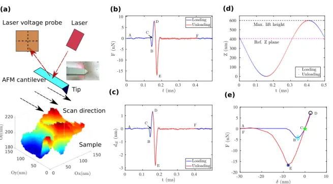
The experimental characteristics and output of the AFM PF-QNM mode are briefly
84
described in Fig. 1. The laser spot is focused on the surface of the cantilever beam
85
(Fig. 1a) and the associated probe measures the laser shifting voltage (LSV) over
86
time, δV (x, t) at a given pixel on the surface described by the in-plane position
87
vector x = (x, y). After a proper calibration process (usually performed on a
non-88
deformable sapphire sample), the bending stiffness of the cantilever κ and the sensitivity
89
of the cantilever deflection γ are estimated assuming a linear elastic, pure-bending
90
response. This allows to directly associate the LSV measurement to the reaction force by
91
F (x, t) = κδV (x, t) (Fig. 1b) and the cantilever deflection as ddf = γδV (x, t)(Fig. 1c).
92
The actual indentation depth δ(x, t) of the cantilever tip is given as the difference of
93
the prescribed vertical displacement of the cantilever Z (Fig. 1d) and the cantilever
94
deflection as ddf, δ(x, t) = Z − ddf.
95
Use of δ, instead of Z or of time t, allows for the influence of topography to be erased
96
for the most part. Fig.1e shows a representative force-penetration, F − δ, response at a
97
fixed position (pixel) x. The paths A→B→C→D (blue line) and D→E→F (red line)
98
correspond to the loading and unloading response, respectively.
99
The entire F − δ response may then be divided in four main regimes (Fig. 1e):
100
– Regime I: A→B→C . As the tip approaches the surface of the specimen, an
101
unstable jump towards contact occurs. The first force minimum during loading at
102
B is used as a conventional definition of contact, and thus as an estimate of surface
103
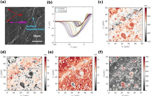
topography. However, because of the intrinsically unstable character of this
“snap-104
in” and its associated hysteresis [37], this commonly adopted definition appears to be
105
delicate, and may intermingle topography with surface force gradients. An alternative
106
more rigorous definition of topography may be obtained with regard to point C, where
Sample -30 -20 -10 0 10 -20 -15 -10 -5 0 5 10 0 0.1 0.2 0.3 0.4 -3 -2 -1 0 1 0 0.1 0.2 0.3 0.4 -15 -10 -5 0 5 10 Laser Tip Laser voltage probe
AFM cantilever Scan direction Sample (a) (b) (d) (e) (c)
Figure 1: PeakForce QNM AFM mode. (a) AFM PeakForce QNM mode: a prescribed displacement loading is repeated in every pixel along the scanning direction; a laser beam reflected by AFM cantilever, is measured by a photo-diode delivering a laser shifting voltage (LSV), which can be converted in cantilever tip position and force at each instant in time t. (b) The deflection force F vs. time t, (c) cantilever deflection ddf vs. time t, (d) total vertical displacement of the cantilever Z vs. time t, (e) deflection force F vs. actual indentation depth δ = Z − ddf. The markers denote the different regimes discussed in the main text.
the tip is in contact with the surface exerting a zero overall applied force. Thus the
108
surface elevation δe(x) at a spatial point x is obtained by the implicit equation
109
F (x, δe(x) = 0) = 0 . (1)
110
– Regime II: C→D. As the cantilever is pushed towards the surface, the force turns
111
from attractive (before point C) to repulsive (after point C) and reaches a maximum at
112
point D.
113
– Regime III: D→E. The tip is then withdrawn (unloading), and the response is
114
that of a (visco)-elastic adhesive contact. Adhesion can be characterized through the
115
pull-out force F reached at point E in the F − δ curve (dark blue star symbol).
116
– Regime IV: E→F. Complete retraction of the tip is mainly dominated by the
117
mechanical instability of tip detachment from the surface, similar to Regime I, but with
118
a higher amplitude because of adhesion.
119
One often assumes that the sample remains purely elastic during the unloading cycle
120
D→E, so that an effective apparent Young’s modulus can be estimated, using either a
121
Hertz or a Sneddon contact model. Nonetheless, if nonlinear and/or viscous effects are
122
present, this analysis can lead to erroneous results, as is the case here especially in the
123
second PDMS-CIP sample.
3. Proper Orthogonal Decomposition
125
This section discusses in some detail the proper orthogonal decomposition (POD)
126
analysis used to analyze the force-indentation data obtained from the PF-QNM AFM
127
mode. Initially introduced in Ref. [38] to study turbulence, the POD is a powerful
128
and elegant method for data analysis aimed at obtaining low-dimensional approximate
129
descriptions of a large data-set.
130
Specifically, in the present work, the force-indentation response is collected in a
131
matrix form F(xi, δj) written in index notation as Fij. This matrix is sampled at
132
each pixel position, xi, (i = 1, .., Nx with Nx denoting the number of pixels) and each
133
indentation depth, δj (j = 1, .., Nδ with Nδ denoting the dimension of the indentation
134
discretization). It should be noted here that linear interpolation between subsequent δj
135
is required in general to obtain intermediate data necessary for the subsequent processes.
136
The POD analysis allows then to separate the matrix F into a set of orthonormal basis vectors (the POD modes) for representing a given data in the form
F(x, δ) = Nδ X n=1 λ(n)U(n)(x)W(n)(δ), or Fij ≡ Nδ X n=1 λ(n)Ui(n)Wj(n). (2) Here, W(n) ∈ RNδ represents the elementary force-indentation mode (normalized as 137
kW(n)k = 1‡), U(n) ∈ RNx is the spatial modulation of this elementary response 138
(normalized as kU(n)k = 1) and λ(n) is a global modal amplitude. At this stage, no
139
approximation is involved, and for all data series F(x, δ), such an exact space-indentation
140
decomposition always exists (but is not unique).
141
Then, one may easily show that both the spatial and the force modes are orthogonal, i.e.,
U(n)· U(m) = W(n)· W(m) = δ(nm) (3)
with δ(nm) = 1 if n = m and 0 otherwise. From the orthonormality conditions, the
following relations can be readily derived
λ(n)U(n)= F W(n) (4) λ(n)W(n)= U(n)F (5) Finally, the eigenvalues can be used to evaluate the relative “energy”, τn, of the
n−th POD mode as τn = (λ(n))2 P m(λ(m))2 . (6)
The most important property of the POD (that can be chosen as a definition) is
142
the fact that modes can be ordered in terms of their significance for representing the
143
‡ We use a standard definition of the Euclidean vector norm kAk =√A · A, where A is a vector of any finite dimension.
data. Then, one may retain only a very small number of those modes to approximate
144
the original response. Both U(n) and W(n) as well as the number, N N
δ, of those
145
retained modes are determined so that the norm of the difference between left and right
146
hand side terms of Eq. (2) is minimized for any choice of N.
147
From the algorithmic point of view, λ(n)appear as eigenvalues sorted in descending
order, whereas either U(n) or W(n) are the associated eigenvectors. Hence, the
truncation of the above relation (Eq. 2) after the first N < Nδ modes,
e FN ≡ N X n=1 λ(n)U(n)(x)W(n)(δ), (7) provides the best approximation of the original data in a least squares sense for a given
148
number of modes. As a result, the POD offers a simple way of compressing the data to
149
a low dimensional space, while guaranteeing the optimality (or minimal loss) of such an
150
approximation.
151
To estimate the accuracy of the approximate description obtained by the POD truncation, conventionally the residual ρi at every spatial position xi can be computed
as ρi(xi) ≡ ρi = Nδ P j=1 (Fij − ( eFN)ij)2 Nδ P j=1 (Fij)2 , i = 1, .., Nx. (8) 152
4. Patch-test: LDPE nano deposits on a PS film
153
First, a sample made from low density polyethylene (LPDE) well-separated nanopods
154
deposited on a polystyrene (PS) substrate is considered (Fig. 2)§. This sample serves
155
as a patch test in our work since it is commonly used to calibrate AFM tips
(RTESPA-156
150 type). For the patch-test, a ROI area of S = 5 × 5 µm2 is scanned with a spatial
157
resolution of 64 × 64 points and a frequency of acquisition 2 kHz.
158
Fig. 2b shows the force-indentation response for twenty random selected pixels
159
inside the ROI. It is clear that the corresponding force-indentation response can be
160
divided into two main data-groups: the first one exhibits a stiff response with low
161
adhesion and negligible viscosity, whereas the second one shows a softer response and
162
with high adhesion and viscosity (as indicated by the hysteresis during unloading).
163
It is essential to point out that even if the PF-QNM mode is controlled to reach a
164
predefined maximum contact force, this is in practice unattainable, as the scan frequency
165
and the complex topography prevent this condition from being accurately satisfied. As
166
a consequence, neither the force range nor the indentation interval are kept constant
167
§ The SEM image does not correspond exactly to the area analyzed by the AFM. Yet, it validates qualitatively the AFM results.
from pixel to pixel, and thus, for a fair comparison of responses at different pixels, one
168
must crop the raw recorded data to a well defined indentation or force level.
169 (a) 5μm LDPE PS Surface Imperfections 1μm 0 1 2 3 4 5 0 1 2 3 4 5 1 2 3 4 5 6 (c) (f) (i) (d) (e) (g) (h) -30 -20 -10 0 10 -30 -20 -10 0 10 -30 -20 -10 0 10 -30 -25 -20 -15 -10 -5 0 5 10 (b) 0 1 2 3 4 5 0 1 2 3 4 5 0.012 0.014 0.016 0.018 0.02 0.022 0 1 2 3 4 5 0 1 2 3 4 5 -0.05 -0.04 -0.03 -0.02 -0.01 0 0.01 0 1 2 3 4 5 0 1 2 3 4 5 -0.1 -0.05 0 0.05 0.1
Figure 2: (a) SEM image showing LDPE nanopods deposited on PS substrate and surface imperfections. (b) Arbitrarily selected force-indentation response at various pixels (continuous lines represent tip approach and dashed lines tip retraction). (b) Force-indentation curve during retraction; the rectangle indicates the region selected for POD analysis. (d) First POD mode spatial mode revealing the phases (e) Second POD mode revealing more subtle information such as PS-LPDE interfaces. (c) Third POD mode showing higher order features related to surface roughness. (g) Residual error resulting by keeping only the first three modes to describe the force-indentation response at each pixel. (h) Subspace generated by the first three POD modes [U(1); U(2); U(3)]. (i) Contour of the frequency of points in the subspace [U(1), U(2)].
In this regard, for the patch test, the force-indentation response is analyzed
170
only during unloading, i.e., Regime III, as shown by the cropping window in Fig. 2c
171
(approximately −15 nm . δ . 5 nm. The contact response is initially (visco)elastic
and subsequently adhesive between the tip and the sample. This implies that our phase
173
segmentation is done for this specific part of the F −δ response and has to be interpreted
174
as such.
175
Subsequently, the cropped force-indentation data points are decomposed into N
176
POD (proper orthogonal decomposition) modes as described by Eq. (7). We show next
177
that the first few POD modes can reproduce most of the complete F − δ response by
178
evaluating the relative power of each POD mode τn in the original data is evaluated via
179
Eq. (8).
180
Fig. 2(d-f) shows the first three POD spatial modes U(n)(x
i), n ≤ 3, ranked
181
from higher to lower value of τn. These first three POD modes represent 96% of
182
the original measured F − δ response, leading respectively to the values, τ1 = 0.75,
183
τ2 = 0.17, and τ3 = 0.04. The first POD mode U(1) captures remarkably well the phase
184
distributions (PS in gray and LDPE in light red in Fig.2d) as the primary information
185
of the mechanical response. The second mode, U(2), (Fig. 2e) reveals the next level of
186
information. In particular, light gray areas at the PS-LPDE interfaces indicates that
187
the mechanical properties in those regions are somewhat different. Finally, the third
188
mode U(3) describes even higher order information that do not affect the first order
189
effects such as the contact laws and material stiffness (Fig. 2f). For instance, the U(3)
190
map reveals regions with steep slopes, such as a scratch at the north-west side, which
191
correlates well with similar defects revealed in the SEM image (Fig.2a).
192
The contributions of higher POD modes, n > N, are negligible as compared to the
193
first three ones and lead mostly to a pure noise map. In this view, the residual ρ can
194
be computed, to highlight pixels where the mechanical response is not very accurately
195
accounted for with the number of POD modes used (Fig. 2g). For a more quantitative
196
analysis, Fig.2h shows the distribution of data in the subspace [U(1); U(2); U(3)], where
197
pixels are grouped into clusters. This allows the segmentation of the different phases and
198
the identification of one or more interfacial regions. Focusing further in the subspace
199
[U(1); U(2)] (Fig.2i), a 2D-histogram shows the statistical frequency of points having a
200
given value of U(1)and U(2). Two main phases characterized by their mean response and
201
deviations are very clearly highlighted making mechanically-based segmentation quite
202
simple.
203
5. Carbon-Iron particles with PDMS binder
204
The second analyzed sample is a composite material consisting of a polymer matrix
205
(PDMS) and mechanically stiff, fairly spherical carbonyl-iron particles (CIP) with mean
206
radius of about ∼ 3 µm. The results from the built-in QNM results are first shown
207
in Fig. 3 to reveal the complexity of the analyzed sample. Subsequently, in Fig. 4, we
208
analyze the date using the proposed POD method.
209
As seen in Fig. 3a obtained by SEM, the white spots represent the reflections from
210
the CIP, whereas the surface of the composite material is marked by multiple line defects.
211
For the AFM analysis, a surface of 50 µm2 is scanned using the PF-QNM mode with a
definition of 128 × 128 points, and a frequency of 2 kHz. The scanned region is selected
213
intentionally such that one of the surface imperfections is present in the ROI.
214
As easily observed in Fig.3b, and unlike the previous ideal patch-test, the variation
215
of the force-indentation curves exhibits a continuous pattern and a marked presence of
216
viscosity and adhesive behavior. As a consequence, it is extremely difficult to segment
217
and identify the underlying phases via a direct pixel-to-pixel analysis. In particular,
218
as highlighted in Fig. 3c, a marked surface imperfection is observed inside the ROI
219
(highlighted in dark color expanding from south-west to north-east). Due to the sharp
220
change in topography and difference in effective contact surface, at these locations,
221
both the maximum of indentation depth and adhesion are quite different than either
222
the PDMS or the CIP response, and thus it is likely to be misinterpreted as a third
223
phase. In the following, the results obtained from our POD proposed approach will be
224
shown and compared with the standard PF-QNM ones.
225 -100 -50 0 -30 -20 -10 0 10 20 0 10 20 30 40 50 0 10 20 30 40 50 470 480 490 500 510 10μm (b) CIP PDMS Surface Imperfections (a) 0 10 20 30 40 50 0 10 20 30 40 50 10 20 30 40 50 0 10 20 30 40 50 0 10 20 30 40 50 10 15 20 25 0 10 20 30 40 50 0 10 20 30 40 50 0 100 200 300 400 500 600 700 (c) (d) (e) (f)
Figure 3: (a) SEM image showing carbonyl iron particles (CIP) embedded in a PDMS matrix, and surface imperfections. (b) Arbitrarily selected force-indentation response at various pixels (continuous lines represent tip approach and dashed lines tip retraction). (c) Topography map using our proposed definition; (d)-(f) Bruker’s PF-QNM built-in results maximum indentation; (d) Maximum Indentation (e) Adhesion (f) Apparent modulus using Sneddon model;
Following the same POD procedure presented in the previous section, a window is
226
selected in the unloading Regime III (Fig.4a) with δ ranging from ∼ −45 nm to ∼ 10 nm.
227
In this initial data-set, after the POD analysis, the first three modes are retained, as
228
shown in Fig.4(b-d). Their contribution amounts to τ1 = 0.91 > τ2 = 0.04 > τ3 = 0.03,
229
respectively, describing approximately 98% of the power of the original F − δ data.
(b) (a) 0 10 20 30 40 50 0 10 20 30 40 50 -0.04 -0.03 -0.02 -0.01 0 0.01 0.02 (c) (d) (f) -60 -40 -20 0 20 -30 -25 -20 -15 -10 -5 0 5 10 15 0 10 20 30 40 50 0 10 20 30 40 50 0 0.05 0.1 0.15 0 10 20 30 40 50 0 10 20 30 40 50 -0.08 -0.06 -0.04 -0.02 0 0.02 0 10 20 30 40 50 0 10 20 30 40 50 2 4 6 8 10 10-3 U(2) U(1) U(3) CIP clusters (e)
Figure 4: (a) Force-indentation curve during retraction; the rectangle indicates the region selected for POD analysis. (b)-(c) First two POD mode spatial modes revealing clearly the CIP-PDMS phases (d) Third POD mode showing higher order features related to surface roughness.(e) Subspace generated by the first three POD modes [U(1); U(2); U(3)]. (f) 2D histogram of amplitudes in the subspace [U(1), U(2)].
Remarkably, despite the continuous pattern in the F − δ responses (Fig. 4a), the
231
first mode U(1) (Fig.4b) reveals the presence of the PDMS matrix (in red) contrasting
232
with the much smaller amplitude of the stiff CIP phase (in white). In particular, we
233
observe a pronounced clustering of CIP particles in at least four regions that exceed a
234
side length of 10 µm (i.e., 3-4 times the radius if the particle) due to aggregation during
235
the sample fabrication. Fig. 4b illustrates the strength of the AFM-POD analysis as
236
compared with the SEM imaging, wherein such delicate features are much more difficult
237
to obtain.
238
The second mode (Fig. 4c) in the present case does not exhibit substantially
239
different features than the first one. In fact, one may note that the CIP particles
240
now have a much larger weight than the soft matrix, i.e.opposite to the case of the first
241
mode. With our proposed algorithm, the rough surface topography does not appear to
242
bias the phase contrast seen in Fig. 4b and c. By contrast, the surface topography is
243
mingled with the phase contrast in all the different Bruker outputs in Fig. 3. Thus, it
244
may be concluded that in the present examples, the POD analysis is a trustworthy and
245
efficient method for phase segmentation.
246
Finally, the third mode (Fig. 4d) reveals the next order of information, this time
247
highlighting the aforementioned topographical defect (light white color) ranging from
south-west to north-east. In the literature, the influence of topography on apparent
249
adhesion has been intensively studied. A sharp variation in surface curvature often leads
250
to a decrease in adhesion for the same material [39]. This observation is consistent with
251
the results reported here as well as those processed by the Bruker AFM software, in spite
252
of the fact that the first modes were observed to be independent of topography. Hence,
253
the POD analysis appears to be an efficient method for rearranging hierarchically and
254
separately different features in PF-QNM AFM data (phase, topography) according to
255
their contribution in the mechanical signal, allowing analysts to describe each individual
256
aspects or their combination altogether.
257
Focusing, next, on the reduced subspace [U(1); U(2); U(3)] allows to reveal the
258
continuous distribution of the data (Fig. 4e). Given that topography is almost
259
entirely suppressed in the first two POD modes, the subspace [U(1); U(2)], (Fig. 4f),
260
becomes a natural “best-candidate” for the purpose of phase segmentation. Two distinct
261
peaks, corresponding to the two main phases, i.e, PDMS and CIP can be observed.
262
However, the scatter of points and the overlap of the two domains suggests in this
263
case that the transition (in terms of apparent mechanical properties) is progressive. It
264
may be speculated that particles buried at different depth beneath the surface may be
265
responsible for this observation.
266 0 10 20 30 40 50 0 10 20 30 40 50 2 4 6 8 10 B A -60 -40 -20 0 20 -30 -25 -20 -15 -10 -5 0 5 -60 -40 -20 0 20 -15 -10 -5 0 5 10 15 20 (b) (a) (c)
Figure 5: Uncertainty(residual) of reconstruction using the first three POD modes: (a) The residual map ; (b) Comparison between the initial force-indentation curve (plotted in dot blue) and reconstructed curve (plotted in red) at point A (ρ(xA) ' 1%); (c) Comparison between the initial force-indentation curve (plotted in dot blue) and reconstructed curve (plotted in red) at point B (ρ(xB) ' 10%)
Finally, in order to assess the accuracy of the POD reconstruction, we show in
267
Fig. 5a, the residual, ρ, which serves to measure the error induced by the truncation
268
to only the first three modes at each pixel. This measure suggests that CIP clusters
269
may require a finer analysis to be better described. In particular, we select and analyze
270
two points with different residual levels, as shown in Fig. 5a. At point A located in
271
the PDMS matrix (see Fig. 5b), the initial force curve is perfectly reconstructed with
272
an error that is less than 1%. In contrast, at point B located inside a cluster of CIP
273
particles, (Fig.5c), the truncation error (of the order of ' 10%) is mostly concentrated
274
at the maximum pull-out force. One possible explanation is that the error results from
275
the unstable mechanism of ’snap-off’ between tip and sample. However, the hysteretic
mechanism of ’snap-off’ is out of the scope of this study, and thus we did not further
277
attempt to reduce the reconstruction error by introducing additional higher order POD
278
modes.
279
6. Conclusions
280
Accessing complex nano- and microstructural morphologies in heterogeneous media is
281
both a need and a challenge. The recent PF-QNM AFM mode represents a major step
282
forward to provide such fine information, whereby each image pixel is fully characterized
283
by a complete mechanical test. However, the analysis of the resulting large data-sets
284
becomes not only delicate (because of the intrinsic coupling of different mechanical
285
and chemical properties with the topography), but also time-wise prohibitive. This
286
letter has shown that model reduction techniques (such as the POD), can be extremely
287
useful in organizing hierarchically such large data-sets allowing not only to identify
288
a small number of modes expressing the underlying phases but also to offer an easy
289
segmentation of the (mechanically relevant) phases. Starting from the force-indentation
290
response, proper classification may reveal discrete material responses, allowing to extract
291
seamlessly the mechanical, chemical or physical response of each of them. In materials
292
with complex microstructures, the proposed processing may indicate, at first sight,
293
that mechanical properties are continuously varying making a manual identification
294
impossible. The POD method allows to properly identify the data points belonging to
295
the same phase and possibly to a transition region between them.
296
We close by emphasizing that the agnostic character of the data processing
297
techniques used here is both a strength — no bias is introduced by enforcing say a
298
contact model that would be unsuited — and a weakness — the physical interpretation
299
(e.g. elastic stiffness, adhesive properties, viscoelasticity) remains in the hand of the
300
user. However, this interpretation becomes now substantially easier and more robust
301
since only a reduced subspace of a much lower dimensionality (i.e.modes) needs to be
302
considered.
303
Acknowledgement
304
X.C., S.H. and K.D. would like to thank Becton and Dickinson Corporation (BD) for
305
financing partially this project and Ms. Saphia Ouanani from Bruker Corporation for
306
very useful discussions. K.D. would also like to acknowledge partial support from the
307
European Research Council (ERC) under the European Union’s Horizon 2020 research
308
and innovation program (grant agreement No 636903).
Appendix A. PS-LDPE sample
310
Appendix A.1. Description of the sample
311
The detailed information concerning the sample type PS-LDPE-12M can be found at the
312
following address: https://www.brukerafmprobes.com/p-3724-ps-ldpe-12m.aspx 313
Appendix A.2. QNM properties
314 0 2 4 0 1 2 3 4 5 184 186 188 190 192 (a) 0 2 4 0 1 2 3 4 5 2 4 6 8 10 (b) 0 2 4 0 1 2 3 4 5 1400 1600 1800 2000 2200 2400 2600 (c) 0 1 2 3 4 5 0 1 2 3 4 5 10 15 20 25 (d)
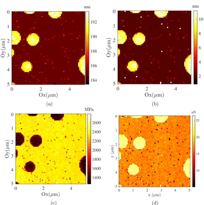
Figure A1: The PF-QNM modality proposed by Bruker provides different mechanical characterizations based on the AFM scan discussed in the main text of the manuscript, relative to the PS-LDPE sample. (a) Topography map; (b) Maximum indentation; (c) Apparent modulus using Hertz model; (d) Adhesion
Appendix A.3. SEM image
315
Figure A2: SEM image (secondary electrons) for the PS-LDPE sample (the dark gray domains are the LDPE nanopods while the PS film substrate appears in light gray
Appendix B. PDMS-CIP sample
316
Appendix B.1. Fabrication process
317
The fabrication procedure of the PDMS+CIP composite can be summarized as follows
318
(see more details in [34]):
319
1. The appropriate amount of CIP powder is mixed along with part A + part B (10:1)
320
of Sylgard 184 in a beaker.
321
2. All ingredients are thoroughly mixed for two minutes at 200 RPM mixer.
322
3. The mixture is put into a vacuum chamber for 34 minutes to remove the entrapped
323
air.
324
4. The degassed liquid mixture is put in an aluminum mold.
325
5. The mold is heated in an oven at temperature T = 373 K for two hours.
326
Appendix B.2. SEM image
327
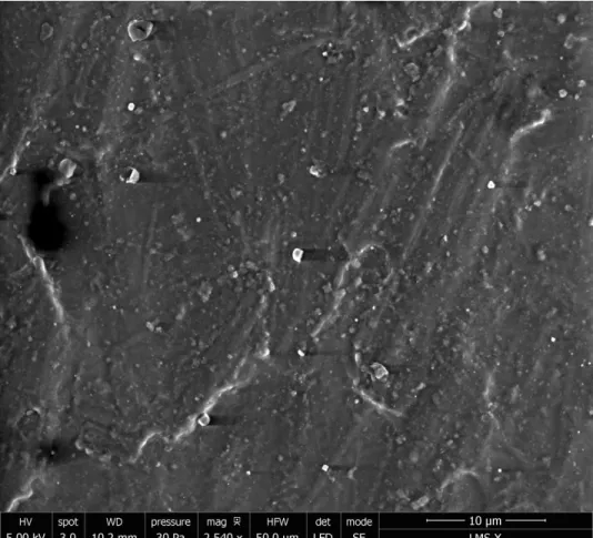
Figure B1: SEM image (secondary electrons) for the PDMS-CIP sample. Bright spots originates from the Carbonyl-Iron particles, while the PDMS shows a darker gray level. A significant roughness of the surface is visible
Appendix C. POD truncation
328
Note that F by construction is not a square (and hence not symmetric). In order to accelerate the computations, we symmetrize F in order to form a square matrix of a minimum dimension that allows to obtain seamlessly the eigenvalues λ(n) and the
eigenvectors W(n). In the present work, we always have N
δ < Nx. As a consequence,
the most efficient symmetrization is obtained by setting [30], M = FT F, or Mij =
Nx
X
k=1
FkjFki. (C.1)
This operation leads to a matrix M of size Nδ×Nδ. The alternative one F·FT would lead
to a matrix size of dimension Nx× Nx > Nδ× Nδ. Using now the definition introduced
in Eq. (2) and simple linear algebra, we can readily get Mij =
Nδ
X
n=1
(λ(n))2Wi(n)Wj(n). (C.2) Thus, use of the symmetric (square) matrix M instead of the non-symmetric F allows to
329
extract in a very simple manner the eigenvalues λ(n)and eigenvectors W(n)by employing
330
any eigensystem algorithm for symmetric real matrices. Once those two quantities are
331
evaluated, one may extract the remaining spatial modes U(n)by use of the orthogonality
332
between the W(n) modes and the direct projection operation, described in Eq. (4).
333
The following algorithm describes the POD operations using this last definition as
334
well as the definitions in Section 3.
335
Algorithm 1: POD truncation
Result: Compute N force and spatial modes using POD Crop Force F and indentation δ data to selected range;
Resample (F, δ) using linear interpolation to a prescribed number of δ points; Force data for all pixels i and δj sampling to be gathered into a matrix Fij;
Compute the square symmetric matrix M = FTF;
Extract the eigenvalues λ(n) of M sorted in decreasing order and the
corresponding eigenvectors W(n) with n = 1, ..., N δ;
Select the appropriate number of modes N << Nδ from the eigenvalue
spectrum;
Compute the corresponding spatial mode U(n)= 1
λ(n)FW
[1] G. Binnig, C. F. Quate, and Ch. Gerber. Atomic force microscope. Phys. Rev. Lett., 56:930–933,
336
Mar 1986.
337
[2] C.F Quate. The afm as a tool for surface imaging. Surface Science, 299-300:980 – 995, 1994.
338
[3] S.N. Magonov, V. Elings, and M.-H. Whangbo. Phase imaging and stiffness in tapping-mode
339
atomic force microscopy. Surface Science, 375(2):L385 – L391, 1997.
340
[4] A Rosa-Zeiser, E Weilandt, S Hild, and O Marti. The simultaneous measurement of elastic,
341
electrostatic and adhesive properties by scanning force microscopy: pulsed-force mode operation.
342
Measurement Science and Technology, 8(11):1333–1338, nov 1997.
343
[5] Lining Lan, Shuhong Xie, Li Tan, and Jiangyu Li. Sol-gel based soft lithography and piezoresponse
344
force microscopy of patterned pb(zrti) microstructures. Journal of Materials Science &
345
Technology, 26(5):439 – 444, 2010.
346
[6] D. Passeri, M. Rossi, and J.J. Vlassak. On the tip calibration for accurate modulus measurement
347
by contact resonance atomic force microscopy. Ultramicroscopy, 128:32 – 41, 2013.
348
[7] T J Young, M A Monclus, T L Burnett, W R Broughton, S L Ogin, and P A Smith. The
349
use of the PeakForceTMquantitative nanomechanical mapping AFM-based method for
high-350
resolution young's modulus measurement of polymers. Measurement Science and Technology,
351
22(12):125703, oct 2011.
352
[8] Kim K. M. Sweers, Kees O. van der Werf, Martin L. Bennink, and Vinod Subramaniam. Atomic
353
force microscopy under controlled conditions reveals structure of c-terminal region of α-synuclein
354
in amyloid fibrils. ACS Nano, 6(7):5952–5960, 2012. PMID: 22695112.
355
[9] Maxim E. Dokukin and Igor Sokolov. Quantitative mapping of the elastic modulus of soft materials
356
with harmonix and peakforce qnm afm modes. Langmuir, 28(46):16060–16071, 2012. PMID:
357
23113608.
358
[10] Moritz Pfreundschuh, David Alsteens, Manuel Hilbert, Michel O. Steinmetz, and Daniel J. Müller.
359
Localizing chemical groups while imaging single native proteins by high-resolution atomic force
360
microscopy. Nano Letters, 14(5):2957–2964, 2014. PMID: 24766578.
361
[11] Hsien-Shun Liao, Ka Kit Lei, and Yu Fang Tseng. High-speed force mapping based on an
362
astigmatic atomic force microscope. Measurement Science and Technology, 30(2):027002, jan
363
2019.
364
[12] Franz J. Giessibl. Advances in atomic force microscopy. Rev. Mod. Phys., 75:949–983, Jul 2003.
365
[13] Yueming Hua. PeakForce-QNM advanced applications training 2014. Technical Support Engineer,
366
2012.
367
[14] G. Smolyakov, S. Pruvost, L. Cardoso, B. Alonso, E. Belamie, and J. Duchet-Rumeau. Afm
368
peakforce qnm mode: Evidencing nanometre-scale mechanical properties of chitin-silica hybrid
369
nanocomposites. Carbohydrate Polymers, 151:373 – 380, 2016.
370
[15] Laida Cano, Daniel Humberto Builes, Sheyla Carrasco-Hernandez, Junkal Gutierrez, and
371
Agnieszka Tercjak. Quantitative nanomechanical property mapping of epoxy thermosetting
372
system modified with poly(ethylene oxide-b-propylene oxide-b-ethylene oxide) triblock
373
copolymer. Polymer Testing, 57:38 – 41, 2017.
374
[16] M. Majewska, D. Mrdenovic, I.S. Pieta, R. Nowakowski, and P. Pieta. Nanomechanical
375
characterization of single phospholipid bilayer in ripple phase with pf-qnm afm. Biochimica
376
et Biophysica Acta (BBA) - Biomembranes, 1862(9):183347, 2020.
377
[17] E. Barthel and S. Roux. Velocity-dependent adherence: An analytical approach for the jkr and
378
dmt models. Langmuir, 16(21):8134–8138, 2000.
379
[18] Gregory D. Jay, Jahn R. Torres, David K. Rhee, Heikki J. Helminen, Mika M. Hytinnen,
Chung-380
Ja Cha, Khaled Elsaid, Kyung-Suk Kim, Yajun Cui, and Matthew L. Warman. Association
381
between friction and wear in diarthrodial joints lacking lubricin. Arthritis & Rheumatism,
382
56(11):3662–3669, 2007.
383
[19] Qunyang Li and Kyung-Suk Kim. Micromechanics of friction: effects of nanometre-scale
384
roughness. Proceedings of the Royal Society A: Mathematical, Physical and Engineering
385
Sciences, 464(2093):1319–1343, 2008.
[20] Uzi Landman, W. D. Luedtke, Nancy A. Burnham, and Richard J. Colton. Atomistic mechanisms
387
and dynamics of adhesion, nanoindentation, and fracture. Science, 248(4954):454–461, 1990.
388
[21] N.A. Fleck, G.M. Muller, M.F. Ashby, and J.W. Hutchinson. Strain gradient plasticity: Theory
389
and experiment. Acta Metallurgica et Materialia, 42(2):475 – 487, 1994.
390
[22] William D. Nix and Huajian Gao. Indentation size effects in crystalline materials: A law for strain
391
gradient plasticity. Journal of the Mechanics and Physics of Solids, 46(3):411 – 425, 1998.
392
[23] G. Haiat, M.C. Phan Huy, and E. Barthel. The adhesive contact of viscoelastic spheres. Journal
393
of the Mechanics and Physics of Solids, 51(1):69 – 99, 2003.
394
[24] E Barthel. Adhesive elastic contacts: Jkr and more. Journal of Physics D: Applied Physics,
395
41:163001, 2008.
396
[25] David Lin, Emilios Dimitriadis, and Ferenc Horkay. Robust strategies for automated afm force
397
curve analysis—i. non-adhesive indentation of soft, inhomogeneous materials. Journal of
398
biomechanical engineering, 129:430–40, 07 2007.
399
[26] David Lin, Emilios Dimitriadis, and Ferenc Horkay. Robust strategies for automated afm
400
force curve analysis—ii: Adhesion-influenced indentation of soft, elastic materials. Journal
401
of biomechanical engineering, 129:904–12, 01 2008.
402
[27] David C. Lin, David I. Shreiber, Emilios K. Dimitriadis, and Ferenc Horkay. Spherical indentation
403
of soft matter beyond the hertzian regime: numerical and experimental validation of hyperelastic
404
models. Biomechanics and Modeling in Mechanobiology, 8(5):345, Nov 2008.
405
[28] B J Briscoe, L Fiori, and E Pelillo. Nano-indentation of polymeric surfaces. Journal of Physics
406
D: Applied Physics, 31(19):2395–2405, oct 1998.
407
[29] Michel Verleysen and Damien François. The curse of dimensionality in data mining and time series
408
prediction. volume 3512, pages 758–770, 06 2005.
409
[30] Anindya Chatterjee. An introduction to the proper orthogonal decomposition. Current science,
410
pages 808–817, 2000.
411
[31] Charles F Van Loan. Generalizing the singular value decomposition. SIAM Journal on numerical
412
Analysis, 13(1):76–83, 1976.
413
[32] Svante Wold, Kim Esbensen, and Paul Geladi. Principal component analysis. Chemometrics and
414
intelligent laboratory systems, 2(1-3):37–52, 1987.
415
[33] K. Danas, S.V. Kankanala, and N. Triantafyllidis. Experiments and modeling of
iron-particle-416
filled magnetorheological elastomers. Journal of the Mechanics and Physics of Solids, 60(1):120
417
– 138, 2012.
418
[34] L. Bodelot, J.-P. Voropaieff, and T. Pössinger. Experimental investigation of the coupled
magneto-419
mechanical response in magnetorheological elastomers. Experimental Mechanics, 58(2):207–221,
420
sep 2017.
421
[35] Erato Psarra, Laurence Bodelot, and Kostas Danas. Two-field surface pattern control via
422
marginally stable magnetorheological elastomers. Soft Matter, 13(37):6576–6584, 2017.
423
[36] E. Psarra, L. Bodelot, and K. Danas. Wrinkling to crinkling transitions and curvature localization
424
in a magnetoelastic film bonded to a non-magnetic substrate. Journal of the Mechanics and
425
Physics of Solids, 133:103734, 2019.
426
[37] Sebastian Rützel, Soo Il Lee, and Arvind Raman. Nonlinear dynamics of atomic force microscope
427
probes driven in lennard jones potentials. Proceedings of the Royal Society of London. Series
428
A: Mathematical, Physical and Engineering Sciences, 459(2036):1925–1948, 2003.
429
[38] K. K. Nomura and S. E. Elghobashi. The structure of inhomogeneous turbulence in variable
430
density nonpremixed flames. Theoretical and Computational Fluid Dynamics, 5(4):153–175,
431
Nov 1993.
432
[39] T. Stifter, E. Weilandt, O. Marti, and S. Hild. Influence of the topography on adhesion measured
433
by sfm. Applied Physics A, 66(1):S597–S605, Mar 1998.