HAL Id: hal-01571623
https://hal-mines-paristech.archives-ouvertes.fr/hal-01571623
Submitted on 4 May 2018
HAL is a multi-disciplinary open access
archive for the deposit and dissemination of
sci-entific research documents, whether they are
pub-lished or not. The documents may come from
teaching and research institutions in France or
abroad, or from public or private research centers.
L’archive ouverte pluridisciplinaire HAL, est
destinée au dépôt et à la diffusion de documents
scientifiques de niveau recherche, publiés ou non,
émanant des établissements d’enseignement et de
recherche français ou étrangers, des laboratoires
publics ou privés.
Introduction to the level-set full field modeling of laths
spheroidization phenomenon in α/β titanium alloys
Danai Polychronopoulou, Nathalie Bozzolo, Daniel Pino Muñoz, Julien
Bruchon, Modesar Shakoor, Yvon Millet, Christian Dumont, Immanuel
Freiherr von Thungen, Rémy Besnard, Marc Bernacki
To cite this version:
Danai Polychronopoulou, Nathalie Bozzolo, Daniel Pino Muñoz, Julien Bruchon, Modesar Shakoor,
et al..
Introduction to the level-set full field modeling of laths spheroidization phenomenon in
α/β titanium alloys.
International Journal of Material Forming, Springer Verlag, 2019, pp.1-11.
�10.1007/s12289-017-1371-6�. �hal-01571623�
1
Introduction to the level-set full field modeling of laths spheroidization
phenomenon in α/β titanium alloys
. D. Polychronopoulou1,a, N. Bozzolo1, D. Pino- Muñoz1, J. Bruchon2, M. Shakoor1, Y. Millet3, C. Dumont4, I. Freiherr von Thüngen5, R. Besnard6 and M. Bernacki1
1
MINES ParisTech, PSL Research University, CEMEF - Centre de mise en forme des matériaux, CNRS UMR 7635, CS 10207, rue Claude Daunesse, 06904 Sophia Antipolis Cedex, France
2
École Nationale Supérieure des Mines de Saint-Étienne. Centre Sciences des Matériaux et des Structures. Département Mécanique et Procédés d'Elaboration. 158 cours Fauriel, 42023 Saint-Etienne Cedex 02, France
3Timet Savoie, 62 avenue Paul Girod, 73400 Ugine, France 4
Aubert & Duval, rue des Villas, 63770 Les Ancizes-Comps, France
5
Safran, SafranTech - Pôle Matériaux et procédés, Rue des Jeunes Bois, Châteaufort, CS 80112, 78772 Magny-Les-Hameaux, France
6
CEA Valduc, 21120 Is-Sur-Tille, France
Abstract. The fragmentation of α lamellae and the subsequent spheroidization of α laths, in α/β titanium alloys, are well known phenomena, occurring during and after deformation. We will illustrate the development of a new finite element methodology to model these phenomena. This new methodology is based on a level set framework modeling the deformation and the ad hoc concurrent or subsequent interfaces kinetics. In the current paper, we will focus on the modeling of the surface diffusion at the α/β phase interfaces and the motion by mean curvature at the α/α grain interfaces.
Keywords: spheroidization, grooving, α laths, surface diffusion,α/β titanium alloys
1 Introduction
Two-phase α/β titanium alloys are materials with numerous applications in different industrial domains, mostly due to their attractive mechanical properties. They present high strength, fatigue and corrosion resistance, low density and good ductility [1].
Titanium alloys exhibit different microstructures depending on the applied thermomechanical path. Spheroidization is a phenomenon observed at α/β titanium alloys with initial stable microstructure of α lamellae inside β grains, during deformation and subsequent thermal treatment. More precisely, during this phenomenon, the fragmentation of α lamellae and the subsequent spheroidization and coarsening of α laths is observed [2].
Spheroidization has received considerable
attention due to its importance in microstructural control. The new spheroidized microstructure shows enhanced strength and ductility; so evidently, this phenomenon raises high interest for the industrial applications [1] [2].
In this paper, we will illustrate a new finite element (FE) methodology in order to model these
microstructural evolutions. Our interest is focused on the predominant mechanisms occurring during the first stages of the spheroidization at the lamellae interfaces without considering the microstructure deformation modeling. The α/α grain interfaces are introduced arbitrarily leading to surface diffusion at the α/β phase interfaces and motion by mean curvature at the α/α grain interfaces. For the purpose of modeling efficiently these interfacial kinetics, a level set framework was introduced. If some studies concerning the full field modeling of coarsening mechanism exist [3], at the authors’ knowledge, the 2D or 3D full field modeling of the first steps of laths spheroidization in α/β titanium alloys is a poorly researched subject on the state of the art.
Some basic cases of surface diffusion will be detailed in order to introduce the numerical methodology. A first case of immersion of a real microstructure from experimental data will be also considered. Finally, a simple case of lamellae splitting due to the interaction of motion by surface diffusion at the α/β interface and motion by mean curvature at the α/α sub-boundaries will be described.
2 The physical mechanisms
According to Semiatin [2], several mechanisms are activated simultaneously during thermomechanical
process leading to spheroidization. During
deformation, it is observed that high angle misorientations are formed inside the α lamellae. Subsequently these misorientations lead to the formation of grooves which imply the penetration of the β phase and lead to the splitting of the α lamellae (see Fig. 1). After the splitting of the α lamellae in smaller parts, a microstructure with α pancake shape particles is obtained. In order to reduce the interfacial energy, the α particles tend towards a shape where the surface area is minimized for a given volume i.e. a spherical one. Then, coarsening (i.e. volume diffusion well known as Ostwald ripening [4]) can take place. To be more precise the spheroidization of the microstructure is a consequent event of the four combined following mechanisms:
crystal plasticity during deformation which introduces the α/α sub-boundaries inside the α lamellae,
motion by surface diffusion at the α/β interfaces,
motion by mean curvature at the α/α
interfaces,
coarsening.
Except the mechanism of crystal plasticity that it obviously occurs during hot deformation, there is no clear distinction of when each one of these mechanisms occurs. At this point it is very important to underline that during spheroidization, we do not have phase fractions evolution.
In the following, we will focus on the mechanisms which are responsible for the splitting of the α lamellae. Grooving is usually initiated by atomic scale processes near the region of α/α grain boundaries and the α/β phases intersection.
These kinetics can be described by motion by surface diffusion at α/β interfaces and motion by mean curvature at the α/α sub-boundaries (Figure 2). These are two competitive mechanisms occurring simultaneously which lead to the lamellae splitting. After the splitting of the α lamellae, surface diffusion at the α/β interfaces of the laths becomes the dominant mechanism before the coarsening by
volume diffusion. Next section illustrates
experimental data describing this sequence.
3 Experimental analysis
Some hot compression tests have been realized (TA-6V alloy) and are detailed below. We have worked with double coned samples and three experiments have been performed (Fig. 3) at 950°C. After the described thermomechanical treatments, a middle cut is realized and the microstructure is observed by SEM-EBSD analysis exactly at the center of the samples corresponding to the maximum strain area.
a)
b)
c)
Figure 1: Splitting of α lamellae into α laths.
20% 30 min Tr
.
950oC 20% 30 min 15 min Tr.
950oC 20% 30 min 1h Tr.
950oCFigure 3: Hot compression experiments ( ̇=0.1 after 30 min of annealing at 950°C: a) 20%, b) 20% and annealing of 15 min at 950°C and c) 20% and annealing of 1h at 950°C.
3
All the experiments start with a thermal treatment of 30 minutes at 950oC in order to reach equilibrium of the volume fraction of the two phases. The first experiment involves only deformation at 950oC ( =20%, ̇=0.1 ) in order to visualize the
microstructure exactly after deformation. Additional 15 min (respectively 1h) of annealing at 950oC is considered for the second (respectively the third) experiment. The purpose is then to quantify the effect of the annealing time concerning the evolution of the microstructure.
Figures 4, 5, 6 illustrate representative SEM images from each stage of the evolution of the microstructure after each experiment. Just after deformation, we can see a not so fragmented microstructure but from the variation of the grey scale color inside the lamellae we can guess a lot of sub-boundaries (Fig. 4). After 15 min of annealing we see changes on the shape but not so sever ones. The shape evolution of the lamellae is obvious but we cannot observe spheroidized microstructure (Fig. 5). After one hour of annealing we can see finally a more spheroidized and coarsening microstructure (Fig. 6).
Figure 4: representative microstructure after 20%
deformation (Fig. 3a experiment).
Figure 5: microstructure after 20% deformation and 15 min
annealing.
Figure 6: microstructure after 20% deformation and 1h
annealing.
In order to discuss quantitativel the microstructure evolutions, we analyze an important number of such representative images in terms of lath area and lath aspect ratio evolutions. Basically by approximating the α laths as ellipses, the aspect ratio is then defined as the ratio between the major axis and the minor one. By measuring approximately 500 α laths for each case we found the mean value of the aspect ratio and of the lath surface at each of the three stages. These results are summarized in Fig.7. They illustrate a fast evolution of the mean shape ratio during the first 15mins with a quasi-stable mean surface value.
During 15 mins and 1h, the mean shape ratio decreases slowly whereas the increase of the mean surface ratio is important. These experimental results are coherent with the involved mechanisms [1] [2]:
After deformation, sub-boundaries inside the lamellae are present and sphereodization is not activated.
During the first minutes of the thermal treatment, surface diffusion and motion by
mean curvature are the predominant
mechanisms which lead to the laths appearance and sphereodization of the laths without a real growth of the mean lath surface (limited effects of the volume diffusion).
After this first step, coarsening becomes the predominant mechanism.
Figure 7: Time evolution of 2D morphological
characteristics of the laths population.
From the observations above, we believe that, modeling the first steps of spheroidization implies the necessity to simulate the boundary motion due to surface diffusion at α/β interfaces and due to the mean curvature at the α/α sub-boundaries. Subsequent modelling of coarsening is of course of prime importance to predict the laths volume time evolution but is only a natural perspective of the present works which are, at yet, dedicated to the two first mechanisms.
Next section illustrates the governing equations of surface diffusion and motion by mean curvature.
3 The physical equations
3.1 Motion by surface diffusion
According to Mullins [5], in order to describe the atoms flow at the α/β interface we can consider a surface flux ⃗
:
⃗ ⃗ (1) where denotes the number of drifting atoms per unit area and ⃗ denotes the average velocity of these drifting atoms. Assuming local equilibrium we can express ⃗ with the Nerst-Einstein formula as following:
⃑⃑
(2)
where denotes the surface diffusivity of the α/β
interface, μ the chemical potential, the Boltzmann constant and T the absolute temperature. The operator corresponds to the surface gradient operator defined as the tangential component of the gradient:
( (3) with the outward-pointing unit vector normal to the surface and
By considering Eq.(1) and Eq.(2), the following equation is obtained:
(4)
Assuming that there is mass conservation, the surface motion can then be described by:
( (5) where
⃑⃑
denotes the normal velocity of the surface and the atomic volume. By combining Eq. (4) and Eq. (5), we obtain:
(6)
with
the surface Laplacian operator (or Laplace-Beltrami operator).
From Eq. (6), it is notable that the normal velocity is associated with the chemical potential of the atoms. Considering κ as the mean curvature (sum of the main curvatures in 3D) and the α/β interface energy
and by ignoring the possible effects of anisotropy, the following relationship is obtained:
. (7)
5
(8)
with
,
the kinetic coefficient. Eq. (8) describes the relation between the motion by surface diffusion and the surface Laplacian of the mean curvature [6-9].3.2 Motion by mean curvature
In order to describe precisely the surface evolution of an α lamella, the influence of the mean curvature should be also considered [8].
The grain boundary energy is indeed important for the lamellae splitting.
The grain boundary energy is given by the well-known Gibbs-Thompson relationship where the normal velocity of the grain boundary is described proportionally to the mean curvature κ:
̌
(9)
with ̌
, where denotes the grain
boundary energy, b is the burgers vector norm associated with the hoping event, ̌ is the Debye frequency, R the gaz constant and Q the apparent activation energy.
3.2 Motion of the interfaces
Surface diffusion and mean curvature motions are taking part simultaneously during the phenomenon of spheroidization. A global velocity combining both of these motions can then be summarized as:
( (10)
with the characteristic function of the α/β phase
interfaces and the characteristic function of the
α/α grain interfaces (Fig. 2).
4 Level set formulation
A level-set model was formulated in order to deal with the topological changes at the α/β interfaces. The level set method was chosen due to its capability to immerse/describe/capture easily in a FE context the interfaces [10-13] and also due to the fact that geometrical quantities as the mean curvature κ and the outside normal n can be obtained as:
‖ ‖ (11) and ( ‖ ‖ (12) with ( ( ( . (13) is then defined over the domain Ω as a signed distance function to the interface Γ of the subdomain of interest that we will denote .
The sign convention of Eq. (11) corresponds to a distance function negative inside and positive outside.
Thus the interface velocity can be rewritten in a level set form as:
⃑⃑ ‖ ‖ ( ( (14) with: { ( { ̌ (
It can also be proved that in the considered level-set formulation [6] [14], can be re-written as:
( ‖ ‖ (‖ ‖ . (17)
The velocity is then defined in the entire domain and corresponds in the vicinity of the zero level-set function of φ, i.e. , to the interfaces velocity [6] [7]. A new numerical methodology of resolution is detailed in the following section concerning the surface diffusion mechanism.
5
A surface diffusion methodology
For the modelling of the induced flow from the surface diffusion mechanism at the α/β interface, a finite element methodology is adopted. At any time t, the transport velocity ⃑⃑ is defined by:
⃑⃑⃑ (
‖ ‖ (‖ ‖ (18)
with . The coefficient is defined as a
constant and it is chosen to neglect any anisotropy concerning the interface energy and the diffusivity. Additionally, isothermal conditions are assumed. The time evolution of ( is then obtained by solving the following convective system:
{ ⃑⃑⃑⃗ ⃑⃑⃑⃑⃑⃗ ( ( ( ) ( ( ) ̅ (19)
The interface can then be obtained at each time step as the 0-isovalue of the distance function and the velocity is updated by following Eq.(18) before the following time step. At the following subsections, more extensive details are given for the resolution algorithm.
5.1. Surface diffusion velocity identification and transport resolution
The methodology used to obtain the surface diffusion velocity is based on the finite element based strategy introduced by Bruchon et al. in [6] [17].
Indeed, as P1 description of the LS is considered in the proposed methodology, one of the basic issues in the problem of surface diffusion is that the velocity is defined by the Laplacian of the curvature, which means that the velocity is a function of the fourth order spatial derivative of φ. The numerical strategy proposed by Bruchon et al. consists to solve this problem by considering a “regularized” formulation. More precisely Eq.(18) is solved in a weak form by using a FE formulation. Further information can be found in [6] [17].
5.2. Convection-Reinitialization methodology By assuming the appropriate calculation of the surface velocity, the traditional strategy of convection and subsequent reinitialization steps is used. The main idea is to solve the advection equation and to rebuild the metric properties of the level-set function in order to keep a distance function (‖ ( ‖ at least near the interface ( . Classical approaches consist in solving, separately, the convective part and the reinitialization part thanks to the resolution of a classical Hamilton-Jacobi system [13] or to adopt an unified advection and renormalization methodology by solving one single equation based on a smooth description of the level-set [16]. Here, a new approach is proposed.
This new approach is based on a separate resolution of the transport and of the reinitialization part. Convective equation is firstly solved thanks to a stabilized P1 solver (SUPG or RFB method). Then, a parallel and direct reinitialization algorithm detailed in [19], which has been proven to be extremely fast and accurate, is used. In this algorithm, the ( interface is firstly discretized into a collection of segments (respectively triangles in 3D) and the nodal values of the level-set function are then updated by finding the nearest element of the collection and calculating the distance between the considered node and this nearest element. This method takes advantage of a space-partitioning strategy using k-d tree and an efficient bounding box strategy enabling to maximize the numerical efficiency for parallel computations.
Moreover, this methodology presents two other interest:
-it enables to avoid the validation/calibration of unphysical parameters necessary to reinitialize the LS function [13] [17],
-it enables to obtain directly an exact P1 description of [20] before to solve Eq. (18) rather than following the classical less precise methodology where the normal is computed by performing a P1 interpolation of the first derivative of the level-set function.
6
First academic case
In this section we examine an ellipsoid shape under surface diffusion. We want to test the efficiency of the proposed formulation for a simple case with an analytical solution. Considered computational domain is a 1mm x 1mm square centered in (0,0). An initial
ellipse (a=0.3mm and b=0.2mm) of
equation ⁄ ⁄ is considered. Of
course, this shape is going to evolve towards a circle shape while conserving its area. Thus limit radius, i.e. limit value of a and b is given by the value √ .
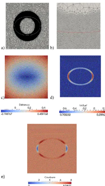
Initially, in order to test the efficiency of the approach without dealing with the effect of the meshing and remeshing in the results, a fixed mesh is considered during simulations. An initial isotropic mesh adaptation is considered in a ring centered in
(0,0) and defined as mm in order
to keep a very fine mesh, defined as h in Table 1, in all the zone crossed by the zero isovalue of the level-set function during the simulation. The figure 8 illustrates the FE mesh used (a), a zoom on the FE mesh (b), the initial distance function field (c), the curvature field near the interface (d) and the normal
b)
d)
7
velocity field near the interface obtained initially thanks to the FE resolution of Eq. (18) (e). Red or white line corresponds to the initial ellipse interface (0 isovalue of the level-set function).
a) b)
c) d)
e)
Figure 8. First academic case: the FE mesh used (a), zoom
on the FE mesh at the interface between coarse and fine mesh (b), the initial distance function field (c), near the interface (d) and near the interface (e).
In all simulations is assumed to be
homogeneous and equal to . Exact velocity of the point (a(t),0) is known [17] and given by:
⃑⃑⃑⃑⃗( ( ) ⃗ ( ⃗ (20) Hence a(t+dt) can be easily evaluated thanks to a
forward Euler method:
( ( ( (21) and b(t+dt) can be easily obtained by verifying the
area conservation at anytime:
( ( ( ( ⁄ (22) This method is then used with a time step of 1ms to evaluate the “exact” evolution of a and b values
during the shape evolution. Concerning FE
simulations, at each time step, the positions of (a(t),0) and (0,b(t)) are determined on the zero-isovalue of the distance function and then compare to the “exact” solution. Final time of all simulations is fixed to 1s.
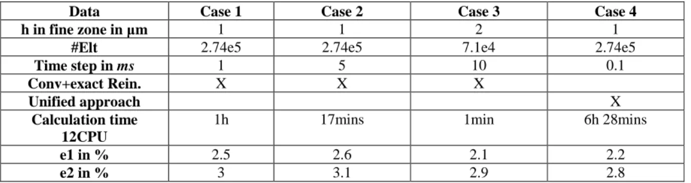
Table 1 summarizes all the parameters (time step, mesh size in the fine mesh zone, number of elements of the used mesh, method used), the CPU time of the simulations and the corresponding precision of the results obtained concerning the positions of (a(t),0) for by using the unified convective-renormalized approach described in [16][17] and the new one proposed here with different time step and h values. These cases are representatives of an important number of other performed simulations. Errors are defined as:
‖ ( ( ‖ ‖ ( ‖ ∑ | | ∑ | | (23) ‖ ( ( ‖ ‖ ( ‖ √∑ ( ) √∑ (24)
where i denotes the discretization in time.
From different simulations (Cases 1 to 4 of Table 1 are representatives), we can summarize the following comments:
-Considering the precision of a(t) predictions (see and errors on Table 1), both approaches are relevant to model surface diffusion. Figure 9 illustrates, at t=0.2s and t=1s, the difference of the exact interface and the results obtained with the Case1.
-The time step of the Case4 ( ) is the maximal value usable for and the unified formulation to avoid numerical instabilities. Such instabilities were not identified for the new proposed approach even for important time step and mesh size (Case 3 for example).
-As illustrated in Table 1, calculation time of the new proposed approach is then clearly very attractive comparatively to the unified approach.
-Even for the new proposed approach, decreasing the and values below, respectively, and seem not improve the results quality ( It can be explained by the fact that the residual error is due to the FE resolution of Eq. (18).
Figure 9: Comparison at t=0s, t=0.2s and t=1s of the exact
solution (red lines) and the Case 1 0-isovalue (blue lines).
7
Second academic case: volume
loss and mesh adaptation
Next, we consider a more realistic shape of a long ellipse with a=0.5mm and b=0.1mm and mesh adaptation. Indeed, in order to obtain acceptable calculation time to model surface diffusion of complex microstructure a fixed meshing strategy as the one of the previous section is not an option. A meshing and remeshing strategy must be used.
To begin with, two metric based meshing strategies associated with the MTC topological mesher were tested. MTC is a P1 automatic remesher based on elements topology improvement that was developed for Lagrangian simulations under large strains [18]. This tool was extended to anisotropic mesh adaptation [18], for which it was extensively used in context of FE microstructure description [6] [12] [13] [16] [17] [19].
The first metric considered, is the metric described in [16]. This metric enables to obtain isotropic or anisotropic (in the normal direction of the interface) fine mesh in the vicinity of the interface without considering its curvature. In this paper, isotropic adaptation was considered (Method 1 in Table 2).
The second metric considered, is based on an a priori error estimator linking the interpolation error on
the LS function to its gradient vector and hessian matrix. As already described, these variables allow to obtain the normal vector to the interface and its main curvatures. Using these data, a metric field can be built in order to obtain a fine mesh size in the vicinity of the interface depending on local curvature [21] (Method 2 in Table 2).
Simulation and data results are reported in Table 2 for both meshing/remeshing methods. The “Conv + exact Reinit” strategy was used. Final time of both simulations is fixed to 1s. As the mesh size near the interface is of the same order than the mesh size used in Case1 and Case2, same precision could be expected. However, remeshing is also synonymous of diffusion concerning the FE fields carrying the interface at each remeshing operation necessary to follow interface motion. Then, volume conservation was tracked for these cases.
Results described in Table 2 illustrate that the mesh adaptation techniques come with good precision and fast calculation times. Meshing adaptation based on the curvature enables to obtain a very good conservation of the volume. This aspect will be of course very important for real configurations where the initial thin shape of the α lamellae implies very high ratio between the minimal and the maximal values of the interface curvature. So, this meshing strategy in terms of metric seems particularly indicated.
Data Case 5 Case 6
h in fine zone in μm 1 1
#Elt <10000 <10000
Time step in ms 1 1
Conv+exact Rein. X X
Calculation time
12 CPU 1min 1min
Remeshing method Method 1 Method 2
Volume loss in % 7.5 1
Table 2. Summarized data and results with mesh adaptation.
If the results described previously in terms of calculation time and precision could be sufficient to study the surface diffusion of one thin ellipse, it seems clear that to further improve our numerical
Data Case 1 Case 2 Case 3 Case 4
h in fine zone in μm 1 1 2 1
#Elt 2.74e5 2.74e5 7.1e4 2.74e5
Time step in ms 1 5 10 0.1
Conv+exact Rein. X X X
Unified approach X
Calculation time 12CPU
1h 17mins 1min 6h 28mins
e1 in % 2.5 2.6 2.1 2.2
e2 in % 3 3.1 2.9 2.8
9
framework, it is important to deal with real 2D or 3D configurations.
In order to face this problem, we adopt a new topological mesher, Fitz, developed by Shakoor et al. [21]. With Fitz, a body fitted meshing and remeshing is possible while using complex metric as previously described. It was then proved in [22] that this new mesher associated with a volume conservation constraint which is compatible both with implicit and body-fitted interfaces, the modification of the interface due to remeshing can be delayed enough so that a Lagrangian Level-Set method becomes more than interesting compared to an Eulerian Level-Set
method, even when large deformations or
displacements occur.
First tests are very promising, allowing in the Case6 configuration to obtain a precision of 2%
concerning the volume conservation with a
calculation time of 30s on 12 CPU. Figure 10 illustrates a result obtained with this numerical framework for a “a=0.5mm and b=0.05mm” configuration.
Moreover we anticipate with this mixed implicit/explicit description of the interfaces an easier coupling between surface diffusion at the α/β interfaces and motion by mean curvature at the α/α grain interfaces.
Figure 10: A “a=0.5mm and b=0.05mm” configuration with
a mixed implicit/explicit description of the interfaces: (top) initial distance function field and the obtained interfaces (white lines) at t=0s, 0.2 s and 1s. (Bottom) Zoom on the conform mesh at t=0.2s, the interface is defined by the red line.
9 Surface diffusion in real
α/β
microstructures
Having tested the validity of the surface diffusion solver in simple configurations, we consider now a more complex one. The FE immersion of a real microstructure, from our experimental images, is investigated.
The considered microstructure of size , described by the Fig. 11, is one similar to the configuration of the Fig. 5 (20% of deformation and 15 min of annealing). This configuration is interesting as splitting can be considered as achieved (see section 3). Binarized version (see Fig. 12) of the microstructure described by Fig. 11 and the signed distance function of the laths was obtained thanks to the ImageJ software and immersed in an initial FE mesh thanks to our FE C++ library CimLib [15]. Some laths, near of the domain boundaries, were deleted in order to avoid border effects.
A first Eulerian Level-Set framework “Conv + exact Reinit“simulation has been considered with
representative physical parameters [2]. We
t=0s
t=0.2s t=1s
Figure 11: α/β microstructure after 20% of deformation and 15 min of annealing.
experienced some difficulties regarding the shape evolution of the interface during the simulation. Having numerous laths interacting very quickly under surface diffusion, lead to oscillations of the interface and severe volume loss.
From the other hand, performing the same simulation with the Lagrangian Level-Set framework based on Fitz methodology, lead to much more reasonable results considering the shape evolution of the lamellae and volume loss as illustrated by the time evolution of Fig. 13. The size of the mesh elements was fixed to close to the lath interfaces
and to otherwise (see Fig. 14). The time
calculation was 2 hours for 12 CPUs. The volume loss from the beginning of the process to the end was limited to 2%. More quantitative validations of these simulations and discussions of the A and B coefficient values will be detailed in a forthcoming publication.
Interestingly, laths coalescence events are observed during surface diffusion. It is logical as one level-set function is considered for all the laths (as in [3] in context of phase field description of the interfaces). However, at the authors knowledge, this kind of evolutions was not reported in the state of the art of α/β titanium alloys during the first steps of the spheroidization. Once again, it seems that consider the role of α/α grain interfaces are of prime importance to predict a realistic evolution of the contacts between the laths during surface diffusion phenomenon.
(a)
(b)
(c
)
(d)
Figure 13: lath evolutions due to surface diffusion: (a)
initial configuration, (b) at , (c) at and (d) at .
Figure 14: Initial mesh adaptation around the α laths (zoom).
10 First simple case of lamellae
splitting:
As already mentioned, two main competitive mechanisms are involved in lamellae splitting. Motion by surface diffusion at the α/β interfaces and motion by mean curvature at the α/α sub-boundaries (see Fig. 2). The numerical framework based on the Fitz meshing/remeshing tools and the enhanced lagrangian methodology is now definitively adopted. The simple configuration of a lath crossed by a α/α grain interface as described by Fig. 15 is considered.
11
Figure 15: Simple case representing a lath crossed by a α/αgrain boundary.
Eq. (17) is taken into account in order to evaluate the global velocity which is used to convect the level-set level-set functions (L1 and L2) describing the two laths. Normalized velocity due to surface diffusion (respectively due to motion by capillarity) is described by the Fig. 16 (resp. the Fig. 17).
Figure 16: Normalized surface diffusion velocity after few
time steps.
Figure 17: Normalized mean curvature velocity after few
time steps.
A realistic ratio between the A and B coefficients is used in order to obtain a representative normalized evolution of the two laths. Fig. 18 illustrates the mesh used for the simulation (conform mesh at the interfaces and a ratio of five between the size of the coarse mesh elements and the fine ones), this figure also clearly illustrates the impact of the mean curvature at the α/α grain boundary concerning the fast appearance of dynamic triple junctions. Even in context of small misorientations and so in context of
weak values of the parameter, the mean curvature
remains extremely high at the initial T-junction between the α/β interface and the α/α interface. Finally Fig. 19 illustrates the splitting of the lamellae in two laths due to surface diffusion and motion by capillarity.
Figure 19: Splitting modeling, from top to bottom: initial
configuration, at , , .
This case demonstrates that the proposed formalism enables to deal with surface diffusion and motion by mean curvature. The volume loss during this simulation was around 1.8%. Current calculations are dedicated to more complex configurations.
10 Conclusions and perspectives
The first steps of a new FE numerical framework dedicated to the modelling of the mechanisms of spheroidization in α/β titanium alloys have been detailed. This numerical framework has been illustrated with some basic numerical cases on surface diffusion of α laths for checking the efficiency of the methodology. Optimal algorithm of resolution and meshing strategies were proposed in terms of precision and calculation time. A new way was also opened by considering a mixed implicit/explicit description of the interfaces with the use of body fitted meshes.
A surface diffusion case on a real microstructure obtained from experimental images was validated in terms of numerical efficiency. We also demonstrate that the proposed formalism enables to simulate lamellae splitting due to the competitive mechanisms of motion by surface diffusion and motion by mean curvature.
The perspectives of this works are numerous. This article illustrates a first step to propose full field simulation of sphereodization and coarsening in α/β
Figure 18: Description of the multiple junctions during
titanium alloys. First of all, more representative simulations in terms of domain size must be realized and the obtained results must be validated with in-situ experimental results. In this context, the coefficients
A, B need to be finely calibrated in order to respect
realistic kinetics. Concerning, the involved
mechanisms, volume diffusion must be added to the global velocity in order to predict realistic volume evolution of the laths during spheroidization. It seems also important to highlight that the proposed methodology is usable in 3D without additional developments. At the authors knowledge, 3D full field modeling of laths for α/β titanium alloys was never addressed. It is then an exciting perspective of these developments. Finally, we plan also to simulate the deformation step thanks to an existing crystal plasticity finite element approach developed in a level-set context [23].
Acknowledgements
The authors would like gratefully to thank AUBERT & DUVAL, CEA, TIMET and SAFRAN for funding this research through the SPATIALES project of the DIGIMU consortium.
Conflict of interest
The authors declare that they have no conflict of interest.
References
[1] Lütjering G. and Williams J. (2007) Titanium. Springer, Heidelberg.
[2] Semiatin S. and Furrer D. (2008) Modeling of
microstructure evolution during the
thermomechanical processing of titanium alloys. Metals Branch, Metals, Ceramics, and NDE Division.
[3] Li X. , Bottler F., Spatschek R., Schmitt A., Heilmaier M. and Stein F. (2017) Coarsening kinetics of lamellar microstructures: Experiments and simulations on a fully-lamellar Fe-Al in situ composite, Acta Materialia, 127: 230-243.
[4] Voorhees P. W. (1985) The theory of Ostwald ripening. Journal of Statistical Physics, 38:231-252. [5] Mullins W. (1958) The effect of thermal grooving on grain boundary motion. Acta Metallurgica 6:414-427.
[6] Bruchon J., Pino Muñoz D., Valdivieso F., Drapier S. and Pacquaut G. (2010) 3D simulation of the matter transport by surface diffusion within a
Level-Set context. European Journal of
Computational Mechanics 19: 281-292.
[7] Derkach V. (2010) Surface evolution and grain boundary migration in a system of 5 grains. M.Sc. thesis, Department of Mathematics, Technion– Israel Institute of Technology.
[8] Derkach V., Novick-Cohen A., Vilenkin A. and Rabkin E. (2014) Grain boundary migration and grooving in thin 3-D systems. Acta Materialia 65: 194-206.
[9] Smereka P. (2003) Semi-implicit level set methods for curvature and surface diffusion motion. Journal of Scientific Computing 19: 439-456.
[10] Osher S. and Fedkiw F. (2001) Level Set Methods: An Overview and Some Recent Results. Journal of Computational Physics 169:463-502.
[11] Sethian J. (1999) Level Sets Methods and Fast Marching Methods. Cambridge Monograph on Applied and Computational Mathematics.
[12] Bernacki M., Logé R. and Coupez T. (2011) Level set framework for the finite-element modelling of recrystallization and grain growth in polycrystalline materials. Scripta Materialia 64:525–528.
[13] Bernacki M., Chastel Y., Coupez T. and Logé R. (2008) Level set framework for the numerical modelling of primary recrystallization in polycrystalline materials. Scripta Materialia 58: 1129-1132.
[14] Burger M., Hausser F., Stocker C. and Voigt A. (2007) A level-set approach to anisotropic flows with curvature regularization. Journal of Computational Physics 225: 183-205.
[15] Digonnet H., Silva L. and Coupez T. (2007) Cimlib: a fully parallel application for numerical simulations based on components assembly. Proceedings of the 9th International Conference on
Numerical Methods in Industrial Forming
Processes.
[16] Bernacki M., Resk H., Coupez T. and Logé R.
(2009) Finite element model of primary
recrystallization in polycrystalline aggregates using a level set framework. Modelling and Simulation in Materials Science and Engineering 17:064006. [17] Bruchon J., Drapier S. and Valdivieso F. (2011) 3D
finite element simulation of the matter flow by surface diffusion using a level set method. International Journal for Numerical Methods in Engineering 86:845-861.
[18] Gruau C. and Coupez T. (2005) 3D tetrahedral, unstructured and anisotropic mesh generation with adaptation to natural and multidomain metric, Computer Methods in Applied Mechanics and Engineering, 194:4951-4976.
[19] Shakoor M., Scholtes B., Bouchard P.-O. and Bernacki M. (2015) An efficient and parallel level
13
set reinitialization method - application to micromechanics and microstructural evolutions. Applied Mathematical Modelling 39:7291-7302. [20] Scholtes B., Boulais-Sinou R., Settefrati A., Pino
Muñoz D., Poitrault I., Montouchet A., Bozzolo N., and Bernacki M. (2016) 3D level set modeling of static recrystallization considering stored energy elds. Computational Materials Science, 122:57-71. [21] Shakoor M., Bernacki M. and Bouchard P.-O.
(2015) A new body-fitted immersed volume method for the modeling of ductile fracture at the microscale: analysis of void clusters and stress state effects on coalescence. Engineering Fracture Mechanics 147: 398-417.
[22] Shakoor M., Bouchard P.-O. and Bernacki M. (2017) An adaptive level-set method with enhanced
volume conservation for simulations in multiphase domains. International Journal for Numerical Methods in Engineering 109:555-576.
[23] Resk H., Delannay L., Bernacki M., Coupez T. and Logé R. (2009) Adaptive mesh refinement and automatic remeshing in crystal plasticity finite element simulations. Modelling and Simulation in Materials Science and Engineering 17:075012.