International Workshop 2007: Advancements in Design Optimization of Materials, Structures and Mechanical Systems 17-20 December 2007 Xi’an, China www.nwpu-esac.com/conference2007/
Practical Computation of Nonlinear Normal Modes
Using Numerical Continuation Techniques
M. Peeters, R. Viguié, G. Kerschen, J.C. Golinval Structural Dynamics Research Group
Department of Aerospace and Mechanical Engineering University of Liege, Liege, Belgium
E-mail: m.peeters, r.viguie, g.kerschen, [email protected]
Abstract
The concept of nonlinear normal modes (NNMs) is considered in the present paper. One reason of the still limited use of NNMs in structural dynamics is that their computation is often regarded as impractical. However, when resorting to numerical algorithms, we show that the NNM computation is possible with limited implementation effort, which paves the way to a practical method for determining the NNMs of nonlinear mechanical systems. The proposed algorithm relies on two main techniques, namely a shooting procedure and a method for the continuation of NNM motions. The algorithm is demonstrated using two different mechanical systems, a nonlinear two-degree-of-freedom system and a nonlinear cantilever beam discretized by the finite element method.
1 Introduction
Nonlinear normal modes (NNMs) offer a solid theoretical and mathematical tool for interpreting a wide class of nonlinear dynamical phenomena, yet they have a clear and simple conceptual relation to the classical linear normal modes (LNMs). The relevance of the NNMs for the structural dynamicist is addressed in Kerschen et al. [1], [2] or in Peeters et al. [3].
However, most structural engineers still view NNMs as a concept that is foreign to them, and they do not yet consider these nonlinear modes as a practical nonlinear analog of the LNMs. One reason supporting this statement is that most existing constructive techniques for computing NNMs are based on asymptotic approaches and rely on fairly involved mathematical developments. In this context, a significant contribution is that of Pesheck [4] who proposed a meaningful numerical extension of the invariant manifold approach.
Algorithms for the numerical continuation of periodic solutions are really quite sophisticated and advanced (see, e.g., Keller [5], Doedel [6], Seydel [7], Nayfeh [8] and the AUTO and MATCONT softwares). These algorithms have been extensively used for computing the forced response and limit cycles of nonlinear dynamical systems [9-14]. Doedel and co-workers used them for the computation of periodic orbits during the free response of conservative systems [15-16].
Interestingly, there have been very few attempts to compute the periodic solutions of conservative mechanical structures (i.e., NNM motions) using numerical continuation techniques. One of the first approaches was proposed by Slater in [17] who combined a shooting method with sequential continuation to solve the nonlinear boundary value problem that defines a family of NNM motions. Similar approaches were considered in Lee et al. [18] and Bajaj et al. [19]. A more sophisticated continuation method is the so-called asymptotic-numerical method. It is a semi-analytical technique that is based on a power series expansion of the unknowns parameterized by a control parameter. It is utilized in [20] to follow the NNM branches in conjunction with finite difference methods, following a framework similar to that of [15].
In this study, a shooting procedure is combined with the so-called pseudo-arclength continuation method for the computation of NNM motions. We show that the NNM computation is possible with limited implementation effort, which holds promise for a practical and accurate method for determining the NNMs of nonlinear vibrating structures.
This paper is organized as follows. In the next section, the two main definitions of an NNM and their fundamental properties are briefly reviewed. In Section 3, the proposed algorithm for NNM computation is presented. Its theoretical background is first recalled, and the numerical implementation is then described. Improvements are also presented for the reduction of the computational burden. The proposed algorithm is then demonstrated using two different nonlinear vibrating systems in Section 4.
2 Nonlinear Normal Modes (NNMS)
The two main definitions of an NNM and their fundamental properties are briefly reviewed in this section. A detailed description of NNMs is given in [2].
2.1 Framework and Definitions
In this study, the free response of discrete conservative mechanical systems with n degrees of freedom (DOFs) is considered, assuming that continuous systems (e.g., beams, shells or plates) have been spatially discretized using the finite element method. The equations of motion are
(1)
where M is the mass matrix; K is the stiffness matrix; x is the displacement vector and fnl is the nonlinear
restoring force vector, assumed to be regular. In principle, systems with nonsmooth nonlinearities can be studied with the proposed method, but they require a special treatment (Leine at al. [21]).
There exist two main definitions of an NNM in the literature due to Rosenberg [22-24] and Shaw et al. [25-28]: Targeting a straightforward nonlinear extension of the linear normal mode (LNM) concept, Rosenberg defined an NNM motion as a vibration in unison of the system (i.e., a synchronous periodic oscillation).
To provide an extension of the NNM concept to damped systems, Shaw and Pierre defined an NNM as a two-dimensional invariant manifold in phase space. Such a manifold is invariant under the flow (i.e. orbits that start out in the manifold remain in it for all time), which generalizes the invariance property of LNMs to nonlinear systems.
At first glance, Rosenberg's definition may appear restrictive in two cases. Firstly, it cannot be easily extended to nonconservative systems. However, as discussed in Lee at al.[18], the damped dynamics can often be interpreted based on the topological structure of the NNMs of the underlying conservative system. Moreover, due to the lack of knowledge of damping mechanisms, engineering design in industry is often based on the conservative system, and this even for linear vibrating structures. Secondly, in the presence of internal resonances, the NNM motion is no longer synchronous, but it is still periodic.
In the present study, an NNM motion is therefore defined as a (non-necessarily synchronous) periodic motion of the undamped mechanical system (1). As we will show, this extended definition is particularly attractive when targeting a numerical computation of the NNMs. It enables the nonlinear modes to be effectively computed using algorithms for the continuation of periodic solutions, which are really quite sophisticated and advanced.
For n-DOF conservative systems with no internal resonances, Lyapunov [30] showed that there exist at least n different families of periodic solutions around the stable equilibrium point of the system. At low energy, the periodic solutions of each family are in the neighborhood of a linear normal mode (LNM) of the linearized system. These n families define n NNMs that can be regarded as nonlinear extensions of the n LNMs of the underlying linear system.
2.2 Fundamental Properties 2.2.1 Frequency-Energy Dependence
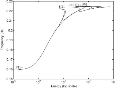
One typical dynamical feature of nonlinear systems is the frequency-energy dependence of their oscillations. As a result, the modal curves and frequencies of NNMs depend on the total energy in the system. In view of this dependence, the representation of NNMs in a frequency-energy plot (FEP) is particularly convenient. An NNM motion is represented by a point in the FEP, which is drawn at a frequency corresponding to the minimal period of the periodic motion and at an energy corresponding to the conserved total energy during the motion. A branch, represented by a solid line, is a family of NNM motions possessing the same qualitative features.
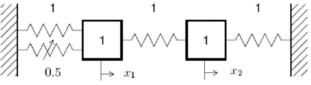
A two-degree-of-freedom (2DOF) system with a cubic stiffness is chosen. The system is depicted in Figure 1, and its NNMs are discussed in more detail in Section 4. The governing equations of motion are
(2) The underlying linear system possesses two (in-phase and out-of-phase) linear modes. The FEP of this nonlinear system, shown in Figure 2, was obtained using the NNM computation method proposed in Section 3. The evolution of NNM motions in the configuration space (i.e., the modal curves) is inset. The backbone of the plot is formed by two branches, which represent in-phase (S11+) and out-of-phase (S11-) synchronous NNMs. They are the continuation of the corresponding LNMs. The letter S refers to symmetric periodic solutions for which the displacements and velocities of the system at half period are equal but with an opposite sign to those at time t=0. The indices in the notations are used to mention that the two masses vibrate with the same dominant frequency. The FEP clearly shows that the nonlinear modal parameters, namely the modal curves and the corresponding frequencies of oscillation, have a strong dependence on the total energy in the system.
Figure 1: Schematic representation of the 2DOF system 2.2.2 Internally Resonant Nonlinear Normal Modes
Another salient feature of NNMs is that they can undergo modal interactions through internal resonances. When carrying out the NNM computation for system (2) at higher energy levels, Figure 3 shows that others branches of periodic solutions, termed tongues, bifurcate from the backbone branch S11+. For instance, unsymmetric periodic solutions are encountered and are denoted by a letter U. On these tongues, denoted Snm and Unm, there exist several dominant frequency components, which results in a n:m internal resonance between the in-phase and out-phase NNMs. These additional branches correspond to internally resonant NNM motions, as opposed to fundamental NNM motions; they have no counterpart in linear systems.
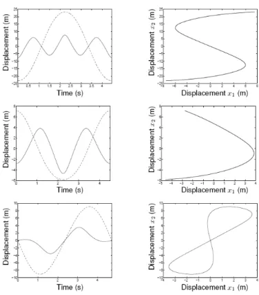
The time series and modal curves corresponding to different NNM motions of system (2) are represented in Figures 4 and 5. Figure 4 shows a fundamental NNM motion on S11+. Three internally resonant NNM motions, namely a motion on S31 and two different motions on U21, are illustrated in Figure 5. The difference between symmetric and unsymmetric NNM motions, as discussed in the previous section, is obvious in this plot. It can also be observed that an NNM motion may take the form of an open or a closed curve in the configuration space. Closed orbits imply phase differences between the two oscillators of the system; i.e., their velocities do not vanish at the same time instant. Interestingly, there exist two different tongues of 2:1 internal resonance in this system, depending on whether the NNM motion is an open or closed orbit in the configuration space. These tongues are coincident and cannot be distinguished in Figure 3.
Figure 2: Frequency-energy plot of system (2). NNM motions depicted in the configuration space are inset. The horizontal and vertical axes in these plots are the displacements of the first and second DOFs, respectively; the
aspect ratio is set so that increments on the horizontal and vertical axes are equal in size to indicate whether or not the motion is localized to a particular DOF.
Figure 4: Fundamental NNM motion on S11+.
Left: time series (−−−: x1(t); - - -: x2(t)). Right: modal curve in the configuration space.
Figure 5: Internally resonant NNMs. From top to bottom: S31, open and closed U21 NNM motions. Left: time series (−−−:x1(t); - - -: x2(t)). Right: modal curve in the configuration space.
2.2.3 Mode Bifurcations
A third fundamental property of NNMs is that their number may exceed the number of DOFs of the system. Due to mode bifurcations, not all NNMs can be regarded as nonlinear continuation of the underlying LNMs, and these bifurcating NNMs are essentially nonlinear with no linear counterparts. Modes generated through internal resonances are one example. Another possible example corresponds to the generation of additional fundamental NNMs. This is discussed at length in Vakakis et al. [31-33].
3 Numerical Computation of NNMS
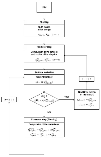
The numerical method proposed here for the NNM computation relies on two main techniques, namely a shooting technique and the pseudo-arclength continuation method. It is summarized in Figure 6.
Figure 6: Algorithm for NNM computation 3.1 Shooting Method
The equations of motion of system (1) can be recast into state space form
(3) where z is the 2n-dimensional state vector in terms of displacement and velocity, and
(4) is the vector field.
The solution of this dynamical system for initial conditions z(0) = z0 is written as z(t) = z(t, z0) in order to exhibit
the dependence on the initial conditions, z(0, z0) = z0.
A solution zp(t, zp0) is a periodic solution of the autonomous system (3) if zp(t, zp0) = zp(t+T, zp0), where T is the minimal period.
The NNM computation is carried out by finding the periodic solutions of the governing nonlinear equations of motion (3). In this context, the shooting method is probably the most popular numerical technique [5, 7, 8, 34]. It solves numerically the two-point boundary-value problem defined by the periodicity condition
(5) H(z0, T) = z(T, z0) – z0 is called the shooting function and represents the difference between the initial conditions
and the system response at time T. Unlike forced motion, the period T of the free response is not known a priori. The shooting method consists in finding, in an iterative way, the initial conditions zp0 and the period T inducing a periodic motion. To this end, the method relies on direct numerical time integration and on the Newton-Raphson algorithm.
Starting from some assumed initial conditions zp0(0), the motion zp(0)(t, zp0(0)) at the assumed period T(0) can be
obtained by numerical time integration methods (e.g., Runge-Kutta or Newmark schemes). In general, the initial guess (zp0(0), T(0)) does not satisfy the periodicity condition (5).
A Newton-Raphson iteration scheme is therefore to be used to correct an initial guess and to converge to the actual solution. The corrections Δzp0(0) and ΔT(0) are found by expanding the nonlinear function
(6)
in Taylor series
(7) and neglecting higher-order terms (H.O.T.).
The initial conditions zp0 and the period T characterizing the periodic solution are computed through the iterative procedure
(8) with
(9) where k is the shooting iteration index. Convergence is achieved when H(zp0(k), T) = 0 to the desired accuracy. In
the neighborhood of the solution, the convergence is fast (i.e., quadratic convergence for an exact evaluation of the Jacobian matrix). However, it should be kept in mind that the Newton-Raphson method is a local algorithm; the convergence is guaranteed only when the initial guess is sufficiently close to the solution.
Each shooting iteration involves the time integration of the equations of motion to evaluate the current shooting residue H(zp0(k), T(k)) = zp(k) (T(k), zp0(k)) – zp0(k). As evidenced by equation (9), the shooting method also requires
the evaluation of the partial derivatives of H(z0, T) = z(T, z0) – z0.
The 2n x 1 vector partial time-derivative of H is given by
The 2n x 2n Jacobian matrix is provided by
(11) where I is the 2n x 2n identity matrix. There are basically two means of computing the Jacobian matrix in the right-hand side of equations (10) and (11).
1. This matrix represents the variation of the solution z(T, z0) at time t when the initial conditions z0 are
perturbed. It can therefore be evaluated through a numerical finite-difference analysis by perturbing successively each of the initial conditions and integrating the equations of motion [8].
2. An alternative computation is obtained by differentiating the equations of motion (3) with respect to the initial conditions z0 (12) It follows (13) with (14)
since z(0, z0) = z0. Hence, the matrix at t = T can be obtained by numerically integrating over T the
initial-value problem defined by the ordinary differential equations (ODEs) (13) with the initial conditions (14).
In addition to the integration of the current solution z(t, z0) of (3), the two previous methods require 2n numerical
integrations of 2n-dimensional dynamical systems, which may be computationally intensive for large systems. However, equations (13) are linear ODEs and their numerical integration is thus less expensive. The numerical cost can be further reduced if the solution of equations (13) is computed together with the solution of the nonlinear equations of motion in a single simulation [35]. We note that the finite-difference procedure is required when g is nondifferentiable, i.e., when the nonlinearities are nonsmooth [8, 35].
In the present case, the phase of the periodic solutions is not fixed. If z(t) is a solution of the autonomous system (3), then z(t+Δt) is geometrically the same solution in state space for any Δt. The initial conditions zp0 can be arbitrarily chosen anywhere on the periodic solution. Hence, an additional condition has to be specified in order to remove the arbitrariness of the initial conditions. Mathematically, the system (9) of 2n equations with 2n+1 unknowns needs a supplementary equation, termed the phase condition.
Different phase conditions have been proposed in the literature [7, 8]. For instance, the simplest one consists in setting one component of the initial conditions vector to zero, as in Arquier et al. [20]. A phase condition particularly suitable for the NNM computation is utilized in the present study and is discussed in Peeters [3]. In summary, the NNM computation is carried out by solving the augmented two-point boundary-value problem defined by
(15) where h(zp0) = 0 is the phase condition.
An important characteristic of NNMs is that they can be stable or unstable, which is in contrast to linear theory where all modes are neutrally stable. In this context, instability means that small perturbations of the initial conditions that generate the NNM motion lead to the elimination of the mode oscillation. Nonetheless, the unstable NNMs can be computed using the shooting procedure.
The stability analysis can be performed when an NNM motion has been computed by the shooting algorithm. The monodromy matrix ΦT of a periodic orbit zp(t, zp0) of period T is defined by its 2n x 2n Jacobian matrix evaluated at t = T
(16) Perturbing the initial conditions with the vector Δz0 and expanding the perturbed solution z(T, zp0 + Δz0) in
Taylor series yields
(17) where Δz(T) =z(T, zp0 + Δz0) - zp(T, zp0).
Equations (17) shows that the monodromy matrix provides the first-order variation of the periodic solution after one period. After m periods, one obtains
(18) The linear stability of the periodic solution calculated by the shooting algorithm is studied by computing the eigenvalues of its monodromy matrix ΦT. The 2n eigenvalues, termed Floquet multipliers, provide the exponential variations of the perturbations along the eigendirections of the monodromy matrix. If a Floquet multiplier has a magnitude larger than one, then the periodic solution is unstable; otherwise, it is stable in the linear sense.
3.2 Continuation of Periodic Solutions
As discussed previously, the conservative system (3) comprises at least n different families of periodic orbits (i.e., NNMs), which can be regarded as nonlinear extensions of the LNMs of the underlying linear system. Due to the frequency-energy dependence, the modal parameters of an NNM vary with the total energy. An NNM family, governed by equations (15), therefore traces a curve, termed an NNM branch, in the (2n+1)-dimensional space of initial conditions and period (zp0, T). As stated before, there may also exist additional NNMs (i.e., bifurcating NNMs) that are essentially nonlinear with no linear counterparts.
In this study, the NNMs are determined using methods for the numerical continuation of periodic motions (also called path-following methods) [7,8, 37]. Starting from the corresponding LNM at low energy, the computation is carried out by finding successive points (zp0, T) of the NNM branch. The space (zp0, T) is termed the continuation space.
Different methods for numerical continuation have been proposed in the literature. The so-called pseudo-arclength continuation method is used herein.
3.2.1 Sequential Continuation
The simplest and most intuitive continuation technique is the sequential continuation method. This procedure is first explained due to its straightforward implementation. Moreover, it provides the fundamental concepts of continuation methods.
The sequential continuation of the periodic solutions governed by (15) is carried out in three steps:
1. A periodic solution (zp0,(1), T(1)) at sufficiently low energy (i.e., in the neighborhood of one LNM) is first
computed using the shooting method. The period and initial conditions of the selected LNM are chosen as an initial guess.
2. The period is incremented, T(j+1) = T(j) + ΔT.
(19)
3. From the current solution (zp0,(j), T(j)), the next solution (zp0,(j+1), T(j+1)) is determined by solving (15)
using the shooting method with the period fixed:
(20) where
The initial conditions of the previous periodic solution are used as a prediction z(0)
p0,(j+1) = zp0,(j). Superscript k is the iteration index of the shooting procedure, whereas subscript j is the index along the NNM branch.
Eventually, one NNM branch is computed. 3.2.2 Pseudo-Arclength Continuation
The sequential continuation method parameterizes an NNM branch using the period T. It has two main drawbacks:
1. Because the convergence of the Newton-Raphson procedure depends critically on the closeness of the initial guess to the actual solution, the sequential continuation requires fairly small increments ΔT. 2. Because the value of the period is fixed during the Newton-Raphson corrections, it is unable as such to
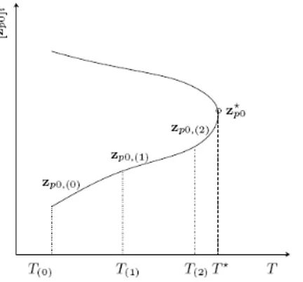
deal with turning points. This is illustrated in Figure 7 where no solution exists for a period larger than the period at the turning point.
For better performance, a continuation algorithm uses a better prediction than the last computed solution. In addition, corrections of the period are also considered during the shooting process. The pseudo-arclength continuation method relies on these two improvements in order to optimize the path following of the branch. Starting from a known solution (zp0,(j), T(j)), the next periodic solution (zp0,(j+1), T(j+1)) on the branch is computed
using a predictor step and a corrector step.
Figure 7: Turning point (T*, z*p0) in the continuation space. Failure of the sequential continuation for T ≥ T*
Predictor step
At step j, a prediction of the next (zp0,(j+1), T(j+1)) is generated along the tangent vector to the branch at the current
point zp0,(j)
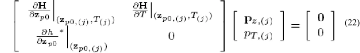
where s(j) is the predictor stepsize. The tangent vector p(j) = [p*(j) pT,(j)]* to the branch defined by (15) is solution
of the system
(22)
with the condition || p(j) || = 1. The star denotes the transpose operator. This normalization can be taken into
account by fixing one component of the tangent vector and solving the resulting overdetermined system using the Moore-Penrose matrix inverse; the tangent vector is then normalized to 1. For illustration, the predictor step is shown schematically in Figure 8.
Figure 8: Pseudo-arclength continuation method: branch (−−−) with a turning point; predictor step (Æ) tangent to the branch; corrector steps (°°°) perpendicular to the predictor step.
Corrector step
The prediction is corrected by a shooting procedure in order to solve (15) in which the variations of the initial conditions and the period are forced to be orthogonal to the predictor step. At iteration k, the corrections
(23) are computed by solving the overdetermined linear system using the Moore-Penrose matrix inverse
(24) where the prediction is used as initial guess.
The last equation in (24) corresponds to the orthogonality condition for the corrector step. Note that the partial derivatives in (24) may be evaluated numerically, as explained previously.
This iterative process is carried out until convergence is achieved. The convergence test is based on the relative error of the periodicity condition:
(25) where ε is the prescribed relative precision.
For illustration, the corrector step is shown schematically in Figure 8. 3.3 An Integrated Approach for the NNM Computation 3.3.1 Basic Algorithm
The algorithm proposed for the computation of NNM motions is a combination of shooting and pseudo-arclength continuation methods, as shown in Figure 6. Starting from the LNM motion at low energy, there are two steps within the algorithm:
1. The predictor step is global and goes from one NNM motion at a specific energy level to another NNM motion at a somewhat different energy level. For an efficient and robust NNM continuation, the stepsize s(j) is to be carefully controlled. A small stepsize leads to a small number of corrector iterations, but it
requires a large number of continuation steps to follow an NNM branch. For a large stepsize, the number of corrector iterations is high, and the convergence is slow. The Newton-Raphson procedure may even break down if the prediction is not close enough to the actual solution. Continuation may therefore be computationally intensive in both cases. The stepsize has to be adjusted, possibly in an automatic and flexible manner. Various adaptive stepsize control procedures are discussed in Seydel [7] and Allgower [37].
2. The corrector step is local and refines the prediction to obtain the actual solution at a specific energy level. The size of the corrections during the corrector step is determined by the solutions of the overdetermined system (24).
NNM Representation
So far, the NNMs have been considered as branches in the continuation space (zp0, T). As explained in Section 2.2.1, an appropriate graphical depiction of the NNMs is to represent them in a FEP. This FEP can be computed in a straightforward manner: (i) the conserved total energy is computed from the initial conditions realizing the NNM motion; and (ii) the frequency of the NNM motion is calculated directly from the period.
Numerical Time Integration
A widely-used method for solving first-order equations such as (3) is the Runge-Kutta scheme. In structural dynamics where second-order systems are encountered, Newmark's family of methods is probably the most widespread technique for solving linear and nonlinear large-scale stiff structural systems [38]. This family of numerical time integration methods is considered in this study.
The precision of the integration scheme, which is chosen by the end-user, directly influences the accuracy of the NNM computation. In fact, the computed solution can be regarded as an exact solution if the sampling frequency used to integrate the equations is sufficiently high. This is practically the only approximation in the proposed algorithm.
Step Control
Unlike sequential continuation, the evolution path of this predictor-corrector method is parameterized by the distance s(j) along the tangent predictor, also referred to as arclength continuation parameter in the literature. As
mentioned previously, the stepsize has to be carefully controlled for a robust and efficient NNM computation. The stepsize control used herein relies on the evaluation of the convergence quality by the number of iterations of the corrector step. The stepsize is controlled so that the corrector step requires on average a desirable number of iterations. Details may be found in Peeters [3].
4 Numerical Experimentations
In what follows, the proposed NNM computation method is demonstrated using two different nonlinear vibrating systems, namely a weakly nonlinear 2DOF system and a nonlinear cantilever beam discretized by the finite element method.
4.1 Weakly Nonlinear 2DOF System
The system is illustrated in Figure 1. The governing equations of motion are
(26) The two LNMs of the underlying linear system are in-phase and out-of-phase modes for which the two DOFs vibrate with the same amplitude. The natural eigenfrequencies are f1 = 0.159 Hz and f2 = 0.276 Hz.
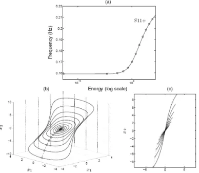
The integrated approach described in Section 3.3 is applied to this system. The computation of the fundamental NNMs is first performed using the modified phase and periodicity conditions. The in-phase backbone S11+ is depicted in Figure 9(a), whereas the out-of-phase backbone S11- is given in Figure 10. Though a large energy range is investigated, these figures show that the continuation method discretizes the two branches using very few points. Large stepsizes are therefore employed, and only a few seconds are required to computed each branch for 100 integration time steps per half period using a 2GHz processor. This is an important feature when targeting a computationally tractable calculation of the NNMs. The two backbones are depicted together in the FEP in Figure 2. The family of in-phase NNM motions is also represented in a three-dimensional projection of the phase space in Figure 9(b) and in the configuration space in Figure 9(c).
The NNM continuation can now be carried out at higher energy levels. The FEP for the in-phase mode is depicted in Figure 11. It can be observed that a recurrent series of tongues of internally resonant NNMs (i.e., S31, S51, S71, etc.) continues the backbone branch S11+ through turning points (fold bifurcations). Due to these turning points, smaller stepsizes are necessary, which renders the tongue calculation more demanding computationally. By contrast, at higher energy on S11-, the 1:1 out-of-phase motion persists, and S11- extends to infinity. The complete FEP calculated using the practical strategy is shown in Figure 12.
Figure 9: In-phase NNM motions on S11+ for the 2DOF system (26). (a) Frequency-energy plot; the computed points are represented by circles. (b) NNM periodic motions represented in a three-dimensional projections of
Figure 10: Frequency-energy plot gathering out-of-phase NNM motions on S11- for the 2DOF system (26). The computed points are represented by circles.
Figure 11: NNMs at high energy for the 2DOF system (26). Left plot: in-phase backbone S11+ and tongues branches (internally resonant NNMs). Right plot: close-up of the recurrent series of tongues (S31, S51 and S71) at high energy. The computed points are represented by circles.
We now move to the general strategy for the computation of unsymmetric NNMs and NNMs represented by a closed curve in the configuration space. These NNMs are generally generated through bifurcations (e.g., symmetry-breaking bifurcations for unsymmetrical NNMs). Because the tangent is not uniquely defined at the bifurcation point, they require a branching strategy to be effectively computed. In this study, a perturbation technique is used to carry out branch switching, once the bifurcation point is located using the Floquet multipliers. The resulting FEP is displayed in Figure 3 and shows two unsymmetrical tongues (U21 and U41). A discussion on the NNM stability may be found in Peeters [3].
4.2 Nonlinear Cantilever Beam
As last example, a planar cantilever beam discretized by 20 finite elements and with a cubic spring at the free end is considered. The geometrical and mechanical properties of the beam are listed in Table 1. This example corresponds to a real nonlinear beam that was used as a benchmark for nonlinear system identification in the framework of the European Action COST F3 [39].
Table 1 : Geometrical and mechanical properties of the planar cantilever beam
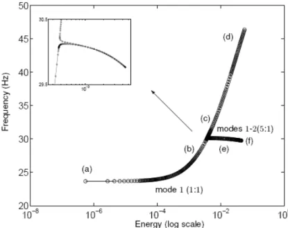
The FEP of the first mode and the related NNM motions are plotted in Figures 13 and 14. The frequency of the NNM motions on the backbone increases with increasing energy levels, which highlights the hardening characteristic of the cubic nonlinearity. The FEP also highlights the presence of one tongue, revealing the existence of a 5:1 internal resonance between the first two modes. When the energy gradually increases along the tongue, a smooth transition from the first to the second mode occurs (see (e) and (f) in Figure 14. The computation of the backbone branch up to the tongue needs 5 minutes with 200 time steps over the half period. Due to the presence of turning points, the computation of the tongue is more expensive and demands 10 minutes.
Figure 14: Maximum amplitudes of the first NNM of the nonlinear beam at different energy levels represented in Figure 13. (a-d): fundamental (1:1) NNMs motions; (e,f): internally resonant NNM motions
between mode 1 and mode 2.
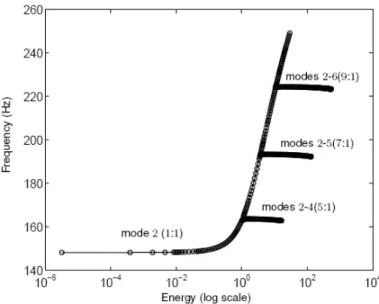
The second NNM is plotted in the FEP of Figure 15. Besides the NNM backbone, three tongues are present. The first tongue corresponds to a 5:1 internal resonance between the second and fourth nonlinear modes of the beam. Similarly, a 7:1 internal resonance between the second and fifth modes, and a 9:1 internal resonance between the second and sixth modes are observed.
Similar dynamics were observed for the higher modes and are not further described herein.
5 Conclusion
In this paper, a numerical method for the computation of nonlinear normal modes (NNMs) of nonlinear mechanical structures has been described. The approach targets the computation of the undamped modes of structures discretized by finite elements and relies on the continuation of periodic solutions. The proposed procedure was demonstrated using two different nonlinear structures, and the NNMs were computed accurately in a fairly automatic manner. Complicated NNM motions were also observed, including a countable infinity of internal resonances and strong motion localization.
This method represents a first step toward a practical NNM computation with limited implementation effort. However, two important issues must be addressed adequately to develop a robust method capable of dealing with large, three-dimensional structures:
• Fundamental NNMs with no linear counterparts (i.e., those that are not the direct extension of the LNMs) have not been discussed herein. These additional NNMs bifurcate from other modes, and a robust branch switching strategy will be developed for their computation.
• The method relies on extensive numerical simulations and may be computationally intensive for large-scale finite element models. As a result, a further reduction of the computational cost is the next objective. To this end, a significant improvement is to use sensitivity analysis to obtain the Jacobian matrix as a by-product of the time integration of the current motion. An automatic time step control, which selects the most appropriate time step in view of the current dynamics, will also be considered to speed up the computations.
The final objective of this research is to implement the method into an industrial finite element program. References
[1] Kerschen, G., Peeters, M., Golinval, J.-C. and Vakakis, A., Nonlinear Normal Modes, Part I: An Attempt to Demystify Them, Proceedings of the International Modal Analysis Conference, 2008.
[2] Kerschen, G., Peeters, M., Golinval, J.-C. and Vakakis, A., Nonlinear Normal Modes, Part I: A Useful Framework for the Structural Dynamicist, Mechanical Systems and Signal Processing, in review.
[3] Peeters, M., Viguié, R., Sérandour, G., Kerschen, G. and Golinval, J.-C., Nonlinear Normal Modes, Part II: Practical Computation using Numerical Continuation Techniques, Mechanical Systems and Signal Processing, in review.
[4] Pesheck, E., Reduced-order modelling of nonlinear structural Systems using nonlinear normal modes and invariant manifolds, Ph.D. thesis, University of Michigan, Ann Arbor, 2000.
[5] Keller, H., Numerical Methods in Bifurcation Problems, Springer-Verlag.
[6] Doedel, E., AUTO, Software for Continuation and Bifurcation Problems in Ordinary Differential Equations, 2007.
[7] Seydel, R., Practical Bifurcation and Stability Analysis. From Equilibrium to Chaos, Springer-Verlag, 1994. [8] Nayfeh, A. and Balachandran, B., Applied Nonlinear Dynamics. Analytical, Computational, and
Experimental Methods, Wiley-lnterscience, Chichester, 1995.
[9] Padmanabhan, C. and Singh, R., Analysis of periodically excited nonlinear-systems by a parametric continuation technique, Journal of Sound and Vibration, Vol. 184, No. 1, pp. 35-58,1995.
[10] Sundararajan, P. and Noah, S., Algorithm for response and stability of large order non-linear Systems — Application to rotor Systems, Journal of Sound and Vibration, Vol. 4, No. 1, pp. 695-723,1998.
[11] Ribeiro, P., Non-linear forced vibrations of thin/thick beams and plates by the finite element and shooting methods, Computers & Structures, Vol. 82, No. 17-19, pp. 1413-1423, 2004.
[12] Govaerts, W., Kuznetsov, Y. and Dhooge, A., Numerical continuation of bifurcations of limit cycles in MATLAB, SIAM Journal on Scientific Computing, Vol. 27, No. 1, pp. 231-252, 2005.
[13] Touzé, C. and Amabili, M., Nonlinear normal modes for damped geometrically nonlinear Systems: Application to reduced-order modelling of harmonically forced structures, Journal of Sound and Vibration, Vol. 298, No. 4-5, pp. 958-981, 2006.
[14] Touzé, C., Amabili, M. and Thomas, O., Reduced-order models for large-amplitude vibrations of shells including in-plane inertia, Proceedings of the EUROMECH Colloquium on Geometrically Nonlinear Vibrations, 2007.
[15] Munoz-Almaraz, F., Freire, E., Galan, J., Doedel, E. and Vanderbauwhede, A., Continuation of periodic orbits in conservative and Hamiltonian Systems, Physica D, Vol. 181, pp. 1-38, 2003.
[16] Doedel, E., Paffenroth, R., Keller, H., Dickmann, D., Vioque, J. G. and Vanderbauwhede, A., Computation of Periodic Solutions of Conservative Systems with Application to the 3-Body Problem, International Journal of Bifurcations and Chaos, Vol. 13, No. 6, pp. 1353-1381, 2003.
[17] Slater, J., A numerical method for determining nonlinear normal modes, Nonlinear Dynamics, Vol. 10, No. 1, pp. 19-30, 1996.
[18] Lee, Y., Kerschen, G., Vakakis, A., Panagopoulos, P., Bergman, L. and McFarland, D., Complicated dynamics of a linear oscillator with a light, essentially nonlinear attachment, Physica D, Vol. 204, pp. 41-69, 2005.
[19] Wang, F. and Bajaj, A., Nonlinear normal modes in multi-mode models of an inertially coupled elastic structure, Nonlinear Dynamics, Vol. 47, pp. 25-47, 2007.
[20] Arquier, R., Bellizzi, S., Bouc, R. and Cochelin, B., Two methods for the computation of nonlinear modes of vibrating Systems at large amplitudes, Computers & Structures, Vol.84, No. 24-25, pp. 1565-1576, 2006. [21] Leine, R. and Nijmeijer, H., Dynamics and Bifurcations of Non-smooth Mechanical Systems,
Springer-Verlag, Berlin, 2004.
[22] Rosenberg, R., Normal modes of nonlinear dual-mode Systems, Journal of Applied Mechanics, Vol. 27, pp. 263-268,1960.
[23] Rosenberg, R., The normal modes of nonlinear n-degree-of-freedom Systems, Journal of Applied Mechanics, Vol. 30, No. 1, pp. 7-14,1962.
[24] Rosenberg, R., On nonlinear vibrations of Systems with many degrees of freedom, Advances in Applied Mechanics, Vol. 242, No. 9, pp. 155-242, 1966.
[25] Shaw, S. and Pierre, C., Nonlinear normal modes and invariant manifolds, Journal of Sound and Vibration, Vol. 150, No. 1, pp. 170-173,1991.
[26] Shaw, S. and Pierre, C., On nonlinear normal modes, ASME Winter Annual Meeting, 1992.
[27] Shaw, S. and Pierre, C., Normal modes for nonlinear vibratory Systems, Journal of Sound and Vibration, Vol. 164, No. 1, pp. 85-124, 1993.
[28] Shaw, S. and Pierre, C., Normal modes of vibration for nonlinear continuous Systems, Journal of Sound and Vibration, Vol. 169, No. 3, pp. 319-347, 1994.
[29] Kerschen, G., Lee, Y. S., Vakakis, A., McFarland, D. and Bergman, L., Irréversible passive energy transfer in coupled oscillators with essential nonlinearity, SIAM Journal of Applied Mathematics, Vol. 66, No. 2, pp. 648-679, January 2006.
[30] Lyapunov, A., The General Problem of the Stability of Motion, Princeton University Press, Princeton, New Jersey, 1947.
[31] Vakakis, A., Manevitch, L., Mikhlin, Y., Pilipchuk, V. and Zevin, A., Normal Modes and Localization in Nonlinear Systems, New York, 1996.
[32] Vakakis, A. and Rand, R., Normal modes and global dynamics of a 2-degree-of-freedom nonlinear-system; Part I: low energies, International Journal of Non-Linear Mechanics, Vol. 27, pp. 861-874,1992.
[33] Vakakis, A. and Rand, R., Normal modes and global dynamics of a 2-degree-of-freedom nonlinear-system; Part II: high energies, International Journal of Non-Linear Mechanics, Vol. 27, pp. 875-888,1992.
[34] Parker, T. and Chua, L., Practical Numerical Algorithms for Chaotic Systems, Springer-Verlag, New York, 1989.
[35] Bruls, O. and Eberhard, P., Sensitivity analysis for dynamic mechanical Systems with finite rotations, International Journal for Numerical Methods in Engineering, Vol. 1, pp. 1-29, 2006.
[36] Mihajlovic, N., Torsional and Lateral Vibrations in Flexible Rotor Systems with Friction, Ph.D. thesis, Eindhoven University of Technology, 2005.
[37] Allgower, E. and Georg, K., Introduction to Numerical Continuation Methods, Classics in applied mathematics, SIAM, 2003.
[38] Géradin, M. and Rixen, D., Mechanical Vibrations, Theory and Application to Structural Dynamics, Wiley, 1994.
[39] Thouverez, F., Presentation of the ECL benchmark, Mechanical Systems and Signal Processing, Vol. 17, pp. 195-202, 2003.