Extension of the group contribution NRTL-PRA EoS for the modeling of mixtures containing light gases and alcohols with water and salts

HAL Id: hal-01703014

https://hal.archives-ouvertes.fr/hal-01703014

Submitted on 12 Feb 2018

HAL is a multi-disciplinary open access

archive for the deposit and dissemination of sci-entific research documents, whether they are pub-lished or not. The documents may come from teaching and research institutions in France or abroad, or from public or private research centers.

L’archive ouverte pluridisciplinaire HAL, est destinée au dépôt et à la diffusion de documents scientifiques de niveau recherche, publiés ou non, émanant des établissements d’enseignement et de recherche français ou étrangers, des laboratoires publics ou privés.

Extension of the group contribution NRTL-PRA EoS for

the modeling of mixtures containing light gases and

alcohols with water and salts

Evelyne Neau, Christophe Nicolas, Laurent Avaullée

To cite this version:

Evelyne Neau, Christophe Nicolas, Laurent Avaullée. Extension of the group contribution NRTL-PRA EoS for the modeling of mixtures containing light gases and alcohols with water and salts. Fluid Phase Equilibria, Elsevier, 2018, 458, pp.194-210. �10.1016/j.fluid.2017.09.028�. �hal-01703014�

A

CCEPTED MANUSCRIPT

_____________________________________________ *corresponding author: evelyne.neau@univ-amu.fr

Extension of the group contribution NRTL-PRA EoS for the modeling of

mixtures containing light gases and alcohols with water and salts

Evelyne Neaua,*, Christophe Nicolasb and Laurent Avaulléec

a

Aix Marseille Univ., CNRS, Centrale Marseille, M2P2, Marseille, France b

MIO (Mediterranean Institute of Oceanography) UMR 7294, Aix Marseille Université, France c _{TOTAL S.A. - CSTJF, Av. Larribau, Pau, France}

Abstract

The offshore exploitation of petroleum fluids in normal conditions of pressure and temperature of transport and in presence of salt water is concerned with the prevention of gas hydrate formation, generally thanks to continuous injection of inhibitors, or punctual injection of methanol in start-up and shut-down operations. Hence, models of interest should provide both, satisfactory phase equilibrium estimations of hydrocarbon and alcohol mixtures with water and reliable predictions of their behavior in presence of salts.

In this work, the NRTL-PRA EoS is extended to the prediction of phase equilibria in mixtures containing strong electrolytes. The proposed model assumes that the a and b parameters of the cubic EoS only depend on the solvent mole fractions (salt-free), while the g_EoSE excess Gibbs energy describes all the interactions between solvents and ions with only two contributions: the SMR term, specific of "Short and Middle Range" interactions between solvents and salts, and the LR relation proposed by Pitzer-Debye-Hückel, for the description of "Long Range" electrostatic interactions. The proposed electrolyte version of the NRTL-PRA model was successfully extended to the modeling of phase behavior of mixtures of light gases at high pressures (methane, carbon dioxide, nitrogen and hydrogen sulfide) and alcohols (methanol, ethanol and 1-propanol) with water and salts (mainly, ternary mixtures containing sodium chloride). As far as possible, results were compared with those provided, for the same systems, by other literature models (cubic Eos, SAFT and CPA equations).

Keywords: Phase equilibria; EoS/GE approach; NRTL-PRA EoS; Electrolytes; Group contributions.

1. Introduction

Formation of gas hydrates leading to pipeline plugging risk is a major problem in offshore petroleum exploitations in transport conditions of pressure and temperature. Their apparition being commonly solved by injecting inhibitor, particularly methanol during transient operations of start-up or shut-down of the transport facilities, an accurate prediction of phase equilibria in mixtures containing hydrocarbon and methanol with salt water is of great interest for petroleum industry.

Many models were proposed in literature for this purpose, which all consist in introducing additional terms to account for the presence of salts in aqueous phases. Among them, the most

A

CCEPTED MANUSCRIPT

popular derive from the SAFT EoS, such as the ePC-SAFT of Cameretti et al. [1] and SAFT-VRE of Galindo et al. [2], or from the CPA equation, as the eCPA model of Courtial et al. [3]. The extension toward electrolytes mainly consists in introducing a specific term for ions directly in the expression of the global residual Helmholtz energy: Ares= A_{non ionic}res + A_ionres; the additional term usually accounts for both "long range" and "middle range" interactions respectively: by means of the Debye-Hückel term of Pitzer [4], MSA [5] or SR2 [6] equations and the Born model [7].

Regarding models based on cubic EoS, most of them derive from two possible approaches, all of them assuming that the salt is not present in the vapor phase: the "homogeneous approach" (LIQUAC equation of Yan et al. [8] or PSRK-LIFAC model of Li et al. [9] and VTPR-LIFAC equation of Collinet and Gmehling [10]), where a classical EoS is associated with a specific expression of the excess Gibbs energy g_EoSE taking ionic species into account. The second technique, initially proposed by Fürst and Renon [6], is an "intermediate approach" which consists: first, in estimating the compressibility factor Z (without taking account salts) and then, in introducing the previous additional "long range" and "middle range" interactions in the derived residual Helmholtz energy (Vu et al. [11] or Sieder and Maurer [12]); we can only regret that "ionic" interactions are not considered for the estimation of the compressibility factor.

Another approach proposed by Masoudi et al. [13] with cubic EoS assumes that salts are present in all phases; even if this assumption allows much more classical "flash" calculations, it usually leads to hard convergence problems, mainly due to the problematic representation of the "unknown" critical parameters of ions.

The purpose of the present work is to extend the fundamental bases of the NRTL-PRA EoS [14] to the prediction of phase equilibria with mixtures containing strong electrolytes. The proposed model is based on the "homogeneous approach" described previously, assuming also that salts are not present in the vapor phase. The a and b parameters of the cubic EoS only depend on the solvent mole fractions (salt-free), while the g_EoSE excess Gibbs energy describes all the interactions between solvents and ions with only two contributions:

- the SMR term, specific of "Short and Middle Range" interactions between solvents and salts, - the LR relation proposed by Pitzer-Debye-Hückel [4] for the description of "Long Range" electrostatic interactions.

The proposed electrolyte version of the NRTL-PRA model was applied to the modeling of light gases at high pressures (methane, carbon dioxide, nitrogen and hydrogen sulfide) and alcohols (methanol, ethanol and 1-propanol) with water and salts (mainly, ternary mixtures containing sodium chloride).As far as possible, results were compared with those provided, for the same systems,by other literature models (cubic Eos, SAFT and CPA equations).

2. Extension of the NRTL-PRA EoS to mixtures containing electrolytes

The presence of electrolytes in a mixture does not only require a new modeling of the g_EoSE excess Gibbs energy, as in the case of associating compounds, like methanol, for the development of the NRTL-PRA model [14] from the original NRTL-PR equation [15]. Indeed, in addition to the fact that

A

CCEPTED MANUSCRIPT

critical parameters of ions are unknown, it is commonly assumed that salts are not present in the

vapor phase, so that great attention must be paid to the calculation of phase equilibria.

For this purpose, it is worth recalling the general conditions of the modeling of mixtures containing salts:

• Preliminary to the introduction of salts, all phases considered (liquid or vapor), are described by means of the same number of compounds, p_SF ,usually called “solvent” or “salt-free” components,

with the corresponding mole numbers,

i SF n , and fractions, i SF x : 1 / , = SF i i i p SF SF SF SF SF i x n n n n = =

∑

(1)

Phase equilibrium conditions at given temperature and pressure satisfy the system of p_SF equations

(3) described in paragraph 2.1.

• The introduction of salts in the previous mixture always follows the same procedure (Appendix B): a well known amount, m0 , of salt is introduced in a well known amount of

i

SF

n moles of the initial solvent (such as, for instance, the mole number m0 of a given salt per kilogram of water, of solvents, ..). The dissociation of salts into pion ions leads, obviously, to the increased total component number, p_tot= p_SF +p_ion, and mole numbers, ni,, and fractions, xi , of the liquid phase:

/ , =

i i tot tot SF ion

x =n n n n +n and: 1 ion k p ion ion k n n = =

∑

(2)

However, thanks to this procedure, the additional pion variables

k ion

n are only functions of the

SF

p mole numbers,

i SF

n of the “salt-free” components. Hence, the real number of independent variables is still equal to p_SF. Consequently, equilibrium conditions at given temperature and pressure must still satisfy the system of p_SF equations (3). The introduction of salts in the liquid phase “only” modifies the expressions of the excess Gibbs energy g_EoSE model and the derived fugacity coefficients.

2.1- Phase equilibria calculation with mixtures containing salts

First of all, the assumption that salts are not present in the vapor phase means that equilibrium conditions at given temperature T and pressure P,must be restricted to the

i SF

n mole fractions of the salt-free components i present in all phases. In the case of vapor-liquid equilibria (VLE), this leads to solve the following equilibrium conditions:

( ) ( ) ( ) ( ) _{( 1, )} i i L L V V SF i xSF i xSF i p ϕ =ϕ = (3)

where φi is the fugacity coefficient of component i derived, for the NRTL-PRA EoS, from the compressibility factor of the Peng-Robinson EoS [16]:

1 ( ) 1 Z Qη α η = − − , 2 1 ( ) 1 2 Q η η η = + − with: b v η= (4)

A

CCEPTED MANUSCRIPT

in which, the attractive term α is estimated in the EoS/gE formalism using the generalized reference state [17]: 1 1 1 , 0.53 SF SF i i p E p i EoS SF SF i i i i a a g x b x b bRT b RT RT α = =   = = −   =  

∑

∑

(5)

where, ai and bi are estimated from the critical temperature and pressure, Tci and Pci (Appendix A). Hence, salts, the critical parameters of which are unknown, are excluded from the estimation of this part of the compressibility factor Z.

On the other hand, the g_EoSE excess Gibbs energy in Eq. (3) only accounts for components really present in each phase:

vapor phase : g_EoSE ( ,T n_SF) , (nV= n_tot =n_SF) (6)

liquid phase: g_EoSE ( ,T n_SF,n_ion) , (nL= n_tot =n_SF +n_ion) (7)

The general expression of gE_EoS proposed in this work for mixtures containing salts is described in

the next section. However, it can already be evidenced with the above relations, especially for the aqueous liquid phase that contains both solvents and ions, that the estimation of fugacity coefficients from Eq. (3) (it means from only salt-free components) should be undertaken very carefully. Indeed, their right thermodynamic expression derived from the Peng-Robinson EoS (Eq. (4)) is described by the following relation:

, ln ( 1) ln (1 ) ( ) / i SF j i SF i SF n T b n Z Z Q RT b n α ϕ = − − − −η η _∂ _ ∂   (8)

in which the derivatives of the α _{term (Eq. (5)) must be expressed as}

, ( / ) / i SF j E SF EoS SF n T n g RT n _{∂ ∂}   

Appendix B presents, for the aqueous liquid phase, the main steps of the calculation of this derivative starting from the classical derivatives

, ( / ) / j E tot EoS i n T n g RT n _{∂ ∂} 

  of gEoSE ( ,T nSF,nion) (Eq. (7)).

2.2- Excess Gibbs energy g_EoSE for electrolyte mixtures

The NRTL-PRA excess Gibbs energy proposed for the simultaneous prediction of LLE, VLE and hE of hydrocarbon mixtures with associating compounds [14] is extended to mixtures containing salts by modifying the residual excess Gibbs energy as follows:

,

E E E E E E

EoS res diss res SMR LR

g = g + g g =g + g (9) where g_resE and g_dissE represent respectively the residual term, taking account for all component interactions, and the dissociation term relative to the decrease of interactions between associating components during mixings. As outlined in the introduction, the residual term is expressed with respect to two contributions only: the g_SMRE term, specific of "Short and Middle Range" interactions

A

CCEPTED MANUSCRIPT

between solvents and salts, and the g_LRE contribution for the description of "Long Range" electrostatic interactions.

The key point of the Short-Middle-Range excess Gibbs energy proposed in this work:

tot tot p p j j ji E SMR i i ji m m mi i=1 j=1 m x q G g x q x q G Γ =

∑

∑

∑

, Gji =exp

(

Γji/RT

)

(10)

is the representation of all interactions involving "solvents" by means of only one single term.

Indeed, the residual term g_resE of the original model [14,15] was already consistent with the virial expressions considered in literature [8-10,12] for the description of the "Middle-Range" interactions between solvents and ions.

The expressions of surface area factors q_i of pure components i and binary interaction

parametersΓ _ji between components i and j with respect to the model group contribution parameters k

Q and

Γ

_LK are recalled in Appendix C. The introduction of salts requires the following modifications:

• Surface area factors q_i. They are estimated thanks to Eq. (C2), using for solvents the group

parameters of UNIFAC [21, 22]. Regarding ions: we have first selected, for Cl- , the values of parameters Qk and Rk proposed by Larsen et al. [23] and deduced "realistic" estimations for Na+ (about half of Cl- parameter values). Then, accounting for the evolution of the "ionic radius" Irk (published by Shannon [24] and reported in Table 1), the group interaction parameters of anions

and cations were estimated as follows, for instance for the surface area factors:

( / )

anion _Cl anion _Cl

Q =Q − Ir Ir − ,Qcation=Q_Na+(Ircation/Ir_Na+).

The values of all subgroup parameters Qk and Rk are reported in Table 1.

• Binary interaction parameters Γ _ji.The estimation of the new interaction parameters

Γ

_{solvent ion/} was performed, assuming for a given salt (Ck+ Ak-), the rather usual assumptions: (1) no interactions between water and ions:

2 / 2 / 0

H O C H O A

Γ

+ =

Γ

− = , (2) no interactions between ions:

/ 0

C A

Γ

+ − = .

The dependence of interaction parameters with respect to temperature is described in Appendix C; corresponding values of parameters

Γ

_LK(0) ,

Γ

_LK(1) and

Γ

_LK(2) are reported, respectively, in Tables 2a, 2b and 2c.

For the "Long Range" electrostatic interactions, g_LRE , we have considered the modeling proposed by Sieder and Maurer [12] based on the original work of Pitzer-Debye-Hückel [4]:

4 ln(1 ) E x z LR z A I g RT

χ

I

χ

  = −  +    (11)

A

CCEPTED MANUSCRIPT

2 1 ( ) 2 ion k p z z ion ion k k=1 I =I x =

∑

x Z (12)

with, Z_k the charge number of ion k and χ an empirical parameter depending on the solvent properties and expressed with respect to the salt-free mole fractions:

1 ( ) 2 / SF i p SF SF i i x M , M x M χ χ ∗ ∗ = = = =

∑

(13)

The electrostatic properties of the solvent mixture are characterized by means of parameter A_x:

2 1/ 2 3 / 2 0 1 2 ( , ) ( ) ( ) 3 4 a x x SF r N e A A T x v kT π πε ε∗ = = ∗ (14)

with, N the Avogadro's number, va ∗ the molar volume of the salt-free solvent, e the charge of one

electron,

ε

₀the vacuum permittivity of vacuum,

ε

_r∗ the relative permittivity of the salt-free solvent mixture and k the Boltzmann's constant.

The molar volume v∗and the relative permittivity

ε

_r∗ of the salt-free solvent mixture are expressed according to [12], as: 1 SF i p SF i i

v

∗

x

b

=

=

∑

, 1

/

SF i i p r SF i r i

x

b

v

ε

∗

ε

=

=

∑

∗

(15)

The method considered in this work for the estimation of the relative permittivity

ε

_riof compound i

is discussed in paragraph 3; estimated values of εr( )T required for the modeling of mixtures studied in this work are reported in Table 3.

The excess Gibbs energy g_dissE was specially introduced in the NRTL-PRA model [14] in order to allow the simultaneous representation of LLE, VLE, and hE for mixtures containing associating compounds (such as methanol) in presence of heavier non associating compounds (long chain

paraffins, cycloalkanes, ...). During such mixings, the decrease of interactions between the associating components i(asso) leads to a significant variation of the global mole fraction of

polymers: from (₍xi 1)₎ i asso

X = , for the pure associating component, towards X_{i asso( )}, for the global mole fraction xi = xi(asso). The NRTL-PRA model proposed the following expression of this dissociation

excess Gibbs energy :

( 1) 0 ( ) ( ) = ( xi ) E diss i i i i asso i i asso g x X = X E =

∑

− ,

E

i asso0_{( )}

=

∆

G

i0

−

( / z )E (z=10)

2

ii (16)

where, the association energy, E_{i asso}0_{( )}, only depends on the experimental value of the hydrogen bond free enthalpy, ∆G_i0 and the estimation of the energy, E_ii, thanks to the model group contribution parameters (Appendix C).

The global mole fraction X_i of polymers is expressed from the knowledge of the "pseudo equilibrium constant" K_i =exp(−∆G_i0/RT) /gam_i usingthe following equilibrium relations:

A

CCEPTED MANUSCRIPT

1 (1 1)

i i i i

X = X / −K X , X_i1=_(1 2+ K x_{i i})− 1 4+ K x_{i i } 2K x_i2 _i_ (17) and the estimation of the mixture parameter:

( ) ( , / ) i i m m i i m i asso gam x x

σ

σ

≠ = +

∑

(18)

which accounts for the polarity: _{m mk k}

k

P =

∑

ν P and structural parameters r_{m i,} characterizing the mixture components: σ_{m i,} =r_{m i,} (P_i−P_m), _{m ,i mk k k}

k

r =

∑

ν R S ; the values of corresponding parameters

k k

R , S and P_k are reported in Table 1.

It should be recalled that mixtures containing only associating compounds (as methanol, water or other alcohols) are assumed to be miscible mixtures, it means without phase splitting. In this case, it was shown [14] that parameter values of P_m fixed to 1 in Table 1, for these compounds, lead to

0

E diss

g ==== ; in this work, the same condition, P_m=1, was extended to ions.

Until now, the dissociating term of the NRTL-PRA model was only taken into consideration for

mixtures containing methanol, since only them required the simultaneous representation of LLE, VLE, and hE [14]. Consequently, for all solvent mixtures studied in this work (except for methanol with carbon dioxide in presence of water) the estimation of the g_dissE term (Eq. (16)) was not required; for this reason, no value of hydrogen bond free enthalpy, ∆G_i0, was reported in parameter tables.

3. Results and discussion

3.1- Preliminary modeling: mixtures with water and permittivity of pure compounds

The modeling of light gases and alcohols with water and salts required the following preliminary studies.

• Mixtures of light gases with water. The VLE of mixtures of light gas and water was revisited in view of a better representation of high pressure data, taking into account [14] the dependence of group contribution parameters with respect to temperature (Eq.(C-3)). Fig. 1 shows the rather good predictions obtained for methane, carbon dioxide, nitrogen and hydrogen sulfide with water. • Alcohol-water and alcohol-paraffin mixtures. The NRTL-PRA model was also extended [25] to

the modeling of VLE and excess enthalpies hE of alcohol-water and alcohol-paraffin mixtures from ethanol to pentanol. It is worth recalling that, like for methanol [14], higher alcohols were modeled by means of one hydroxyl group "OH" and paraffinic main groups "PAR" (Table 1). As expected, methanol, ethanol, as well as primary and secondary alcohols, were described with specific groups in Tables 2.

• Correlation of the relative permittivityεr( )T . A first study of mixtures containing respectively water and methanol with sodium chloride was performed using classical correlations proposed in literature [26-28]; as illustrated in Figs. 2a and 2b, respectively for these two solvents, a "strange" behavior of ε_r( )T was observed, especially for water, at temperatures greater than 350 K.

A

CCEPTED MANUSCRIPT

Taking into consideration “data” generated from various literature correlations (Chunxi and Fürst [26] for water, Dannhauser and Bahre [27] for methanol and CRC tables [28] for other solvents of interest) a generalized function has been proposed for polar compounds [29]:

2

/ ln( )

r A BT CT D T E T

ε

= + + + + (19)

with two objectives: first, to obtain the best representation of the "experimental domain" defined by the CRC tables (as illustrated, for instance, in Fig. 2a for water and in Fig. 2b for methanol); second, to allow a reasonable extrapolation of the reduced permittivity ε_rat high temperatures, it means up to 600 K (as required for the modeling of methane or carbon dioxide mixtures with water and salts in Figs. 1 and 4); values of parameters A, B, C, D and E for all polar compounds considered in this work are reported in Table 3.

Concerning light gases, for which values of ε_rare known to be "small" and "rather constant" with respect to temperature, we have adopted, as described in Table 3, the values proposed by the CRC tables at a given reference temperature.

3.2- Modeling of mixtures containing sodium chloride

Sodium chloride being the main seawater salt (at around 85% of all salts), a large amount of experimental VLE data was available in literature, especially with methane, carbon dioxide, hydrogen sulfide and methanol. Data referenced in Table 4 only concern the experimental data at pressures up to 600 bar considered for the estimation of the group contribution parameters

(0) (1)

,

LK LK

Γ Γ and Γ_LK(2) (Eq. (C-3)) required for the calculation of the binary interaction parameters

/ Na solvent

Γ

+ and

Γ

_Cl−_/solvent in the gSMRE Gibbs energy (Eq.(10)).

The objective function Fobj minimized was:

(

)

2

(

)

2

(

)

2 1 1 1 1 1 y P T N N N

exp exp exp

obj i i i i i i F ∆P / P ∆T / T ∆y / y = = = =

∑

+

∑

+

∑

(20)

where ∆P, ∆T and ∆y1 are, respectively, the deviations between experimental and calculated values

on bubble points and vapor mole fractions; NP, NT and Ny are the corresponding number of data

points. This led to the following mean deviations reported in Table 4:

1 100 P P N exp i i P / P% P / P N ∆ ∆ = =

∑

, 1 100 NT exp i T i T / T % T / T N ∆ ∆ = =

∑

, _{1 1} 1 100 Ny exp i y i y / y% y / y N ∆ ∆ = =

∑

(21)

Results of the correlation reported in this table evidence that standard deviations must be considered very carefully for VLE data at high pressures, especially for mixtures containing light

gases. For mixtures with alcohols at low pressures, deviations are more reliable and the model provides rather good estimations of VLE data. At the end, these global results led us to consider that the proposed data set was significant enough to provide reliable estimations, especially for the

/ Cl solvent

Γ

− values; hence the estimated group contribution parameters,

Γ

LK, reported in Tables 2a,

A

CCEPTED MANUSCRIPT

Finally, global results were illustrated with figures 3 to 6, where phase diagrams are represented with respect to the salt-free mole fraction x1 of the solvent component (1). The analysis of the various

predictions calls the following remarks.

• Methane: Figs. 3a and 3b illustrate the modeling proposed with the NRTL-PRA model at 408 K; the prediction of VLE data up to very high pressures, about 1400 bar, appears to be rather reliable. The representation proposed by Courtial et al. [3] with the eCPA equation at the same temperature is presented in Fig. 3c ; both models lead to quite similar results.

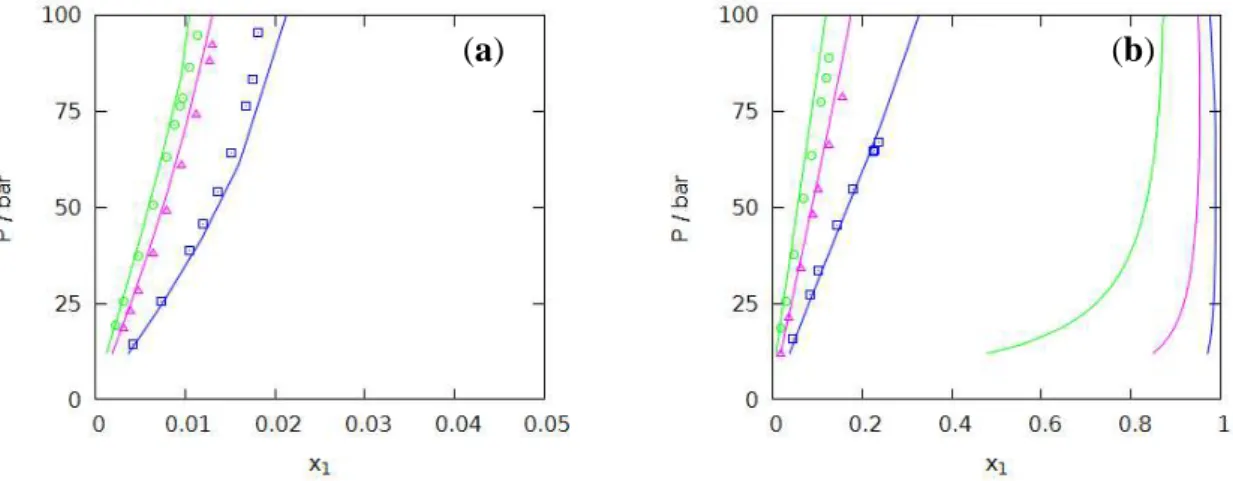
• Carbon dioxide: Fig. 4a presents the NRTL-PRA predictions of VLE from 323 K to 450K, for a molality m0=1.0 mol.kg-1; very good results were thus obtained in these conditions, up to 500 bar.

It should be pointed out that similar results are also previously obtained, for the same range of temperatures and pressures, with other literature models, such as: for cubic EoS, the PSRK-LIFAC [9], VTPR-LIFAC [10] and the extension of the PR EoS to electrolytes proposed by Sieder and Maurer [12]; and, for SAFT equations, the SAFT1-RPM (Ji. et al. [30]) and SAFT-LJ (Sun and Dubessy [31]) models.

Results obtained at 572 K are illustrated in Fig. 4b; for the same amount of salt, the NRTL-PRA equation predicts a closed phase envelope, in agreement with results obtained without salt; however, in this case, this behavior does not agree with the experimental data of Takenouchi and Kennedy [32] which suggest, in the same conditions, an open phase envelope with pressures up to 1500 bar. For this purpose, a comparison with the eCPA model [3] was also performed in Fig. 4c; it can be observed that this modeling follows the tendency suggested by Takenouchi and Kennedy, but, however, with a less favorable behavior of the vapor phase beyond 500 bar.

• Nitrogen and hydrogen sulfide: results presented in Fig. 5 deal with more moderate pressures; even if less meaningful, the proposed correlations are still reasonable. Results obtained with hydrogen sulfide in Fig. 5a are still in agreement with those proposed by Li et al. [9] with the PSRK-LIQUAC model in the same domain.

• Methanol and ethanol: as usual for mixtures containing alcohols, results presented in Fig. 6 correspond to a fixed mole fraction, xsalt , of sodium chloride. Calculations of VLE under 1.0 bar

are quite satisfactory. It should be also noted that curves presented in Fig. 6a for methanol, under atmospheric pressure, are in complete agreement with those proposed, in the same conditions, by Sieder and Maurer [12] by means also of a cubic PR EoS "extended" to electrolytes.

3.3- Prediction of system carbon dioxide-methanol-water-sodium chloride.

• Prediction of VLE data

In order to check the limits of the proposed method, we have considered the quaternary system: carbon dioxide – methanol – water – sodium chloride, with the experimental data of Pèrez Salado Kamps et al. [33], not included in our data base. The authors have performed various sets of measurements corresponding to different values of the solvent composition and amount of salt

introduced in the mixture; the following characteristic parameters were considered:

(2) (2) (3)

/( )

n n n

A

CCEPTED MANUSCRIPT

ρ, represents the “so called” « solute-free solvent mixture composition » and ms isthe molality of

sodium chloride with respect to (methanol+water) mixtures.

Predictions presented in Fig. 7 are also quite good and agree with the curves proposed by Sieder and Maurer [12] for the same system, in the same experimental conditions. Results seem therefore very encouraging for further extensions of the NRTL-PRA model.

• Detailed example of the VLE method.

This quaternary system was also considered in Appendix D for illustrating the calculation method described in section 2. It should be mentioned that, contrary to all other mixtures considered in this work, the system methanol with carbon dioxide in presence of water is the only one which requires the estimation of the g_dissE term (paragraph 2.2).

3.4- Mixtures with other salts

Besides sodium chloride, other salts containing mainly magnesium, calcium and potassium associated with chlorine were also considered as representative of seawater properties. As can be seen in Table 5, which details the VLE data available in literature: the information concerning mixtures of methane with all salts, is rather reasonable; however, for carbon dioxide, ethanol and 1-propanol, experimental data are limited to only two or three salts.

As suggested previously, the modeling of these data only consists in the estimation of the interaction parameters

Γ

_Mg2+_{, Ca}2+_{, K}+_{, Li}+ _{or Br}- _/solvent, accounting for the values of

/ Cl solvent

Γ

− parameters previously determined in section 3.2. Data were regressed in the same way as

for mixtures with sodium chloride (Eq. (20)); deviations thus obtained (Eq. (21)) are given in Table 5 and the corresponding group contribution parameters are reported in Tables 2a, 2b, 2c.

Even if the results presented in Table 5 concern a more restricted range of pressures, similar conclusions to those of Table 4 can be drawn: deviations corresponding to mixtures with methane and carbon dioxide should still be considered carefully; for mixtures with alcohols, results are more significant and satisfactory.

The major results obtained with the various salts are also illustrated with some meaningful figures (Figs. 7-10) and the following remarks.

• Methane: data of methane-water with MgCl2 and LiCl, respectively at 298 K (Fig. 8a) and 313 K

(Fig. 8b), focus rather on moderate pressures (up to 100 bar), compared to those presented in Fig. 3 with sodium chloride. Hence, results are rather good and deviations are similar to those obtained in literature with other salts: CaCl2, in the case of the PSRK-LIFAC [9] model, or LiBr and KBr, my

means of the VTPR-LIFAC [10] equation.

• Carbon dioxide: pressures considered in Fig. 9a, for mixtures containing KCl at 313 K, are much higher (up to 400 bar); the estimation of VLE with CaCl2 (Fig. 9b) at 298 K is still limited at 60

bar. In both cases, the model leads to rather good representations. In this case, we also observed,

with CaCl2, that both NRTL-PRA and PSRK-LIFAC [9] models lead to the similar modeling.

• Ethanol and 1-propanol: data presented in Table 5, respectively for ethanol with LiBr and 1-propanol with KBr, correspond to experimental measurements performed, at each pressure

A

CCEPTED MANUSCRIPT

(Fig. 10a) or temperature (Fig. 10b), for variable values of the molality m0. Hence, both figures

only present the calculated properties with respect to the experimental values. Results remain, however, quite meaningful (less than 2%, even for 1-propanol with KBr). We can also note that other literature results presented with VTPR-LIFAC [10] for ethanol and 1-propanol, with LiCl and LiBr, but under atmospheric pressure, were also rather satisfactory.

4. Conclusion

The purpose of the present work was to extend the fundamental bases of the NRTL-PRA EoS [14] to the prediction of phase equilibria in mixtures containing electrolytes. However, it should be recalled that the presence of electrolytes in a mixture does not only require a new modeling of the

E EoS

g excess Gibbs energy; indeed, not only critical parameters of ions are unknown, but it is commonly assumed that salts are not present in vapor or hydrocarbon liquid phases, so that great

attention must be paid to the calculation of phase equilibria.

In the proposed modeling, the a and b parameters of the cubic EoS only depend on the solvent mole fractions (salt-free), while the g_EoSE excess Gibbs energy is still described with: the residual

term, g_resE , taking account for all component interactions, and the dissociation term, g_dissE , relative to the decrease of interactions between associating components during mixings; nevertheless, as pointed out in paragraph 2.2, for all solvent mixtures considered in this work (except for methanol with carbon dioxide in presence of water) the estimation of the g_dissE term was not required. The presence of electrolytes leads to a major modification of g_resE ; contrary to other cubic EoS, the proposed version describes all the interactions between solvents and ions with only two contributions: the SMR term, specific of "Short and Middle Range" interactions between solvents and salts, and the LR relation of Pitzer-Debye-Hückel [4], for the "Long Range" electrostatic interactions.

The main interest of the proposed method is not only the reduction of the interaction parameters in the SMR term; in fact, the key point of the modeling is that g_SMRE is simply expressed with the original g_resE of the NRTL-PRA model [14,15], since it was already consistent with the virial expressions considered in literature [8-10,12] for the description of the "Middle-Range" interactions between solvent and ions. Thanks to these theoretical bases, it was expected that the modeling of mixtures containing salts would lead, with a lower number of estimated parameters, to more reliable

predictions.

The purpose of this work was, therefore, to verify these assumptions. The following mixtures were considered: light gases at high pressures (methane, carbon dioxide, nitrogen and hydrogen sulfide) and alcohols (methanol, ethanol and 1-propanol) with water and salts. The VLE in presence of sodium chloride and other strong electrolytes (mainly, magnesium, calcium and potassium associated with chlorine) were modeled with the proposed electrolyte version of the NRTL-PRA model. The rather satisfactory modeling obtained using a large data base from open literature can be considered as significant tests for the capacity of the NRTL-PRA equation to represent mixtures

containing light gases and alcohols with water and salts. The analysis of results obtained with other literature models has also shown that:

A

CCEPTED MANUSCRIPT

- concerning other cubic EoS: quite similar results were obtained, at moderate temperatures, for all mixtures investigated. The main interest of the proposed version is, probably that: first, the modeling requires "less regressed" model parameters; second, that it allows rather "safe predictions " at high temperatures and pressures, as for methane and carbon dioxide with water and sodium chloride. - regarding non cubic EoS, as SAFT and CPA versions, rather few papers could be found for the representation of systems considered in the present study, except for carbon dioxide with water and sodium chloride: SAFT [30, 31], in the subcritical domain of salt-free systems, and eCPA [3], at high pressures and temperatures; other papers concerning aqueous mixtures with carbon dioxide (with Brine and sodium chloride [34]) or hydrogen sulfide (PVT properties of imidazolium based ionic liquids [35]) were, obviously, not considered herewith. Nevertheless, with respect to cubic EoS, the great advantage of SAFT versions (SAFT-VRE [2] or ePCA-SAFT [1,36]) is the capacity of predicting a wide field of physical properties (vapor pressure and liquid densities of aqueous solutions with salts, activity coefficients, osmotic pressure ...).

In the present state, results obtained in this work seem very encouraging for further extensions of the NRTL-PRA model. Until now, we have only focused on the representation of VLE with a single electrolyte; the next work will be dedicated: first, to the modeling of LLE and SLE, and then, to the representation of mixtures containing several salts.

The extension of the proposed model to weak electrolytes, would require, for instance with acetic acid, the introduction of an ionization constant [37], but also of chemical equilibrium of dimerization [12, 38], as with associating compounds. Therefore, this development could only be considered in future works.

Acknowledgements

The authors would like to gratefully thank Olivier Baudouin (ProSim) and Isabelle Raspo (M2P2) for valuable discussions.

List of symbols

a attractive term

b covolume

Fobj objective function

G molar Gibbs free energy

K Boltzmann's constant.

Ir ionic radius

m0 molality (with respect to water)

ms molality (with respect to water + methanol)

n mole number

N number of data points

a

N Avogadro's number

P pressure

p component number

A

CCEPTED MANUSCRIPT

R ideal gas constant

Qk,Rk, Sk, Pk NRTL-PRA subgroup contribution parameters

T temperature

v molar volume

Z compressibility factor

x mole fraction

X mole fraction of polymers

y vapor phase composition

Greek letters

α alpha function

ε permittivity

Φ fugacity coefficient

Γji interaction parameter between molecules j and i

ΓLK interaction parameter between main groups K and L

ω acentric factor

ρ solute-free solvent factor

θiK probability that a contact from molecule i involves a main group K

νiK number of main group K in molecule i

Subscript

diss dissociation property

i pure component property

ion number of ions

LR Long Range interaction

obj objective function

P, T, y pressure, temperature, vapor mole fraction

res residual property

salt number of salts

SF salt-free

SMR Short-Middle Range interaction

tot total number of components : SF (solvents) + ions

Superscript

E excess property at constant pressure

APPENDIX A. EoS pure component parameter estimation

The attractive term ai and the covolume bi in Eq. (5) are estimated from the critical temperature and

pressure, Tci and Pci respectively, by the formulae:

( )

2 2 0.45723553 i , 0.07779607 i i i c c i r i c c R T RT a f T b P P = = (A-1)

A

CCEPTED MANUSCRIPT

where Tr is the reduced temperature, Tr =T Tc_i , and f(Tr) is the generalized Soave function [18]:

( )

(

)

2

1 1

r r

f T = +_ m −Tγ _ (A-2)

For hydrocarbons and non associating compounds,we still consider the original Soave function [19] corresponding to γ = 0.5 with the parameter m correlated to the acentric factor ω through the generalized expression proposed by Robinson and Peng [20]:

2 2 3 0.37464 1.54226 0.26992 if 0.49 0.379642 1.48503 0.164423 + 0.016666 if 0.49 m m ω ω ω ω ω ω ω = + − ≤ = + − > (A-3)

On the other hand, for associating compounds, γ and m parameters are estimated with the values previously proposed in [18] to improve vapor pressure representations (γ = 0.65, m = 0.6864 for water and γ= 0.9, m = 0.6969 for methanol).

APPENDIX B. Calculation of partial derivatives in variables (T,nSF) from gEoSE ( ,T nSF,nion)

The modeling of phase equilibria in mixtures containing strong electrolytes assumes that a given amount, n_salt, of a salt (Ck+ Ak-), leading to nions_kof each type k+ and k-, is introduced in nSF moles

of the salt-free solvent. The partial derivatives are estimated as described below.

(1)- Properties of the "solvent+salt" mixture. If

i salt

n is the mole number of salt introduced per mole

of component i of the solvent (mainly water, in classical applications), the total mole numbers of salt and ions are:

1 SF i i p salt salt SF i n n n = =

∑

, 1 ion k p ion ion k n n = =

∑

with : 1 SF k i i p

ion salt salt SF

i

n k n k n n

=

= =

∑

(B-1)

Thus, the excess Gibbs energy g_EoSE ( ,T n_SF,n_ion) proposed in Eq. (7) by the NRTL-PRA model depends on p_tot = p_SF +p_ionvariables representing the mole numbers of “solvent” (nSF) and “ions”

(nion). Nevertheless, as shown in the last term of (B-1), the pion variables

k ion

n are only functions of

the pSF variables nSF_i; hence, the real number of independent variables is the pSF mole numbers

i SF

n of the “salt-free” components.

However, the classical estimation of the partial derivatives,

, ( ) / j E tot EoS i n T n g n _{∂ ∂}    , with respect to

all the mole numbers really present in the liquid phase, does not represent the required derivatives expressed in Eq.(8). The following calculations should be performed for this purpose.

(2)- Derivatives of (n g_{tot EoS}E )with respect to the salt-free mole numbers i SF

n . For the first derivative we get: , ( ) / i SF j E tot EoS SF n T n g n _{∂ ∂}    = ( ) / _, j E tot EoS i n T n g n _{∂ ∂}   

A

CCEPTED MANUSCRIPT

+ , ( ) / _k ( _k / _i) j E

tot EoS ion ion SF

k n T

n g n n n

_{∂ ∂}  _{∂ ∂}

 

∑

(B-2)

with, according to Eq. (B-1) : ( / )

k i i

ion SF salt

n n k n

∂ ∂ = (B-3)

(the same procedure is applied to the second derivatives)

(3)- Derivatives of (n_SFg_EoSE )with respect to the salt-free mole numbers i SF

n . This function is first expressed as: n_SFg_EoSE =(n_SF /n_tot) (n g_{tot EoS}E ) in order to account for the derivatives previously estimated : , ( ) / i SF j E SF EoS SF n T n g n _{∂ ∂}    = ( / ) ( ) / i _, SF j E

SF tot tot EoS SF n T n n _∂ n g ∂n _ + ( / ) / i SF j E

EoS tot SF tot SF _n

g n _∂ n n ∂n _ (B-4)

with : ( / ) / = 1 ( / ) ( / )

i i _{SF j}

j

tot SF tot SF _SF SF tot tot SF

n _∂ n n ∂n _ − n n ∂n ∂n (B-5)

and, according to Eq. (B-1) :

1 ( / ) 1 SF i i p tot SF salt i n n k n = ∂ ∂ = +

∑

(B-6)

Hence, Eq. (B-4) leads to the rigorous derivatives to use in Eq. (8) for the fugacity coefficients. It is also obvious that, for the vapor phase where the lack of salts leads to: n_tot =n_SF, the calculation of above formulae (B-2) and (B-4) is unnecessary, since they are strictly equivalent to the partial derivative , ( ) / j E tot EoS i n T n g n _{∂ ∂}    required in Eq. (8).

APPENDIX C. Group contribution parameter estimation

According to the NRTL-PRA model, binary interaction parameters Γji and Eii in Eqs. (10) and

(16) are estimated with the original group contribution method:

(

)

ji iK jL iL LK K L

Γ

=

∑

θ

∑

θ

−

θ

Γ

, _{ii iK iL LK} K L E =

∑

θ

∑

θ Γ , Γ_KK =0 (C-1)

where θiK is the probability that a contact from a molecule i involves a main group K :

( ) k , ( ) iK ik K i ik K k i k k Q q Q q

θ

=

∑

ν

=

∑

ν

(C-2)

with νik(K) the number of subgroup k belonging to the main group K in a molecule i and q its _i

corresponding surface area factor.

The dependence of group contribution parameters ΓLK with respect to temperature recently

proposed [14] is considered for both solvents and ions:

(0) (1) 0 (2) 0 1 1 LK LK LK LK T T T T Γ =Γ + Γ  −  + Γ  −    _{ } (C-3)

A

CCEPTED MANUSCRIPT

APPENDIX D. Detailed example of the VLE method: system carbon dioxide(1)-methanol(2)

-water(3)-sodium chloride.

Table D details, for one "data point", the various steps of the phase equilibrium calculation method proposed in paragraph 2.1. We consider one point (xSF(1) = 0.0130) of the prediction

described in Fig. 7a for the experimental data of Pèrez Salado Kamps et al. [31] at 313.66 K, with the characteristic mixture parameters proposed by the authors (Eq. (22)) : ρ = 0.049 and ms=1.74. The

exact characteristics of the "selected data point" reported in Table D, are therefore:

T = 313.66 K , x_SF(1) = 0.01300 , x_SF(2) = 0.04830 and x_SF(3) = 0.93870 (D-1) with, for one mole of solvent, n_SF = 1, the following mole number of salt, n_salt = 0.03212, leading thus to:

n_Na+ = = 0.03212 , n_Cl- = 0.03212 and n_tot = 1.06424 (D-2)

The first part of Table D presents the values of the pure compound parameters required, at temperature T , for the modeling: EoS parameters, in Eq.(5), and g_EoSE properties, in Eqs. (10, 15). Only the non zero interaction parameters Γji are reported in this table; the dissociation energy used in

Eq. (16) for methanol is, as proposed in [14]: E_{i asso}0_{( )}= −9980.62 6833.96(298.15 /− T −1).

The following part of the table details, for the liquid phase, the different steps required, according to Appendix B, for the estimation of the partial derivatives of g_EoSE ( ,T n_SF,n_ion)with respect to mole fractions.

A "bubble point" method is then considered for the estimation of the phase equilibrium conditions described in Eq. (3). At the end of the iterative process, the final values of the pressure and salt-free mole fractions of the vapor phase are:

P = 47.672 bar , y_SF(1) = 0.99652 , y_SF(2) = 0.00112 and y_SF(3) = 0.00235 (D-3) The last part of Table D provides, both for the liquid and vapor phases, all the details required for the estimation of the fugacity coefficients in Eq. (8).

It can be seen in this table, that the equilibrium conditions (Eq. (3)) characterized by the “equality”, for all the compounds i, of the products

i

i xSF

ϕ between the liquid and vapor phases, are

very well satisfied. This result is obtained thanks to a "reliable and fast" bubble point algorithm based on the use of "analytical derivatives" (previously verified with numerical tests) and "strict" convergence criterions (∆ ϕ_iL Lx_SFi−ϕ_iV Vx_SFi <10−10) for the resolution of Eq. (3).

References

[1] L.F. Cameretti, G. Sadowski, J.M. Mollerup, Ind. Eng. Chem. Res. 44 (2005) 3355-3362.

[2] A. Galindo, A. Gil-Villegas, G. Jackson, A.N. Burgess, J. Phys. Chem. B 103 (1999)

10272-10281.

[3] X. Courtial, N. Ferrrando, J.C. de Hemptinne, P. Mougin, Geochim. Cosmochim. Acta. 142

A

CCEPTED MANUSCRIPT

[4] K.S. Pitzer, J.Phys.Chem. 77 (1973) 268-277.

[5] F.X. Ball, H. Planche, W. Fürst, H. Renon, AICHE J., 31 (1985) 1233-1240.

[6] W. Fürst, H. Renon, AIChE J. 39 (1993) 335-343.

[7] M. Born, Z. Phys. 1(1920) 45-48.

[8] W. Yan, M. Topphoff, C. Rose, J. Gmehling, Fluid Phase Equilib. 162 (1999) 97-113.

[9] J. Li,, M. Topphoff, K. Fisher, J. Gmehling, Ind. Eng. Chem. Res. 40 (2001) 3703-3710. [10] E. Collinet, J. Gmehling, Fluid Phase Equilib. 246(1-2), (2006), 111-118.

[11] V.Q. Vu, P. Duchet-Suchaux, W. Fürst W., Fluid Phase Equilib. 194-197 (2002) 361-370.

[12] G. Sieder, G. Maurer, Fluid Phase Equilib. 225 (2004) 85-99

[13] R. Masoudi, M. Arjmandi, B. Tohidi, Chem.Eng.Sci., 58 (2003) 1743-1749.

[14] E. Neau, I. Raspo, J. Escandell, Fluid Phase Equilib. 427 (2016) 126-142 [15] J. Escandell, E. Neau, C. Nicolas, Fluid Phase Equilib. 301 (2011) 80-97

[16] D.Y. Peng, D.B. Robinson, Ind. Chem. Fundam. 15 (1976) 59-64.

[17] E. Neau, J. Escandell, I. Raspo, Chem. Eng. Sci. 66 (2011) 4148-4156.

[18] E. Neau, I. Raspo, J. Escandell, C. Nicolas, O. Hernández-Garduza, Fluid Phase Equilib. 276 (2009) 156-164.

[19] G. Soave, Chem. Eng. Sci. 27 (1972) 1197-1340.

[20] D.B. Robinson, D.Y. Peng, Gas Processors Association Research Report, Edmonton-Alberta,

1978.

[21] H.K Hansen, P. Rasmussen, A. Fredenslund, M. Schiller, J. Gmehling, Ind. Eng. Chem. Res., 30

(1991) 2352-2355.

[22] T. Holderbaum, J. Gmehling, Fluid Phase Equilib. 70 (1991) 251-265.

[23] B. L. Larsen, P. Rasmussen, A. Fredenslund, H.K. Hansen, IEC Res, Ind. Eng. Chem. Res, 26

(1987) 2274-2286.

[24] R. D. Shannon, Acta Cryst. A32 (1976) 751-767.

[25] E. Neau, C. Nicolas, L. Avaullée, 29

th

Symposium on Applied Thermodynamics, Bucharest (Romania), 18-21 May 2017.

[26] L. Chunxi, W. Füst, Chem. Eng. Sci. 55 (2000) 2975-2988.

[27] W. Dannhauser, L.W. Bahre, J. Chem. Phys. 40(10) (1964) 3058-3066.

[28] W.M. Haynes, CRC Handbook of Chemistry and Physics, 95th edition (2014-2015).

[29] E. Neau, I. Raspo (to be submitted to Chem. Eng. Sci. 2017).

[30] X. Ji, S.P. Tan, H. Adidharma, M. Radosz, Ind. Eng. Chem. Res. 44 (2005) 8419-8427.

[31] R. Sun, J. Dubessy, Geochim. Cosmochim. Acta. 88 (2012) 130-145.

[32] S. Takenouchi, G.C. Kennedy, Am. J. Sci. 263 (1965) 445-454.

[33] A. Pérez-Salado Kamps, M. Jödecke, J. Xia, M. Vogt, G. Maurer, Ind. Eng. Chem. Res., 45

(2006) 1505-1515.

[34] L.M.C. Pereira, A. Chapoy, R. Burgass, B.Tohidi, Advances in Water Resources 103 (2017)

64-75.

[35] M. Rahmati-Rostami, B. Behzadi, C. Ghotbi, Fluid Phase Equilib. 309 (2011) 179-189.

[36] C. Held, L.F. Cameretti, G. Sadowski, Fluid Phase Equilib. 270 (2008) 87-96.

[37] P. Wang, A. Anderko, R.D. Young, Fluid Phase Equilib. 223(1) (2002) 141-176.

[38] A. Bamberger, G. Sieder, G. Maurer, J.Supercrit.Fluid 17 (2000) 95-110.

A

CCEPTED MANUSCRIPT

[40] S. Takenouchi, G.C. Kennedy, Am. J. Sci., 262 (1964) 10055-10741.

[41] A. Chapoy, A.H. Mohammadi, B. Tohidi, D. Richon, J. Chem. Eng. Data 50 (2005) 1157-1161.

[42] R. Wiebe, V.L. Gaddy, C.J. Heins, Ind. Eng. Chem. 24 (1932) 927-930.

[43] D. Koschel, J.-Y. Coxam, V. Majer, Ind. Eng. Chem. Res. 52 (2013) 14483-14491.

[44] T.N. Kozintseva, Geochem. Int. (1964) 750-756.

[45]

C.W. Blount, L.C. Price, L.M. Wenger, M. Tarullo, Fourth United States Gulf Coast

Geopressured-Geothermal Energy Conference, Research and Development 4.3 (1980) 1225-1262.

[46] W. Yan, S. Huang, E.H. Stenby, Int. J. Greenhouse Gas Control 5 (6) (2011) 1460-1477. [47] S.D. Malinin, N.I. Savelyeva, Geochem. Int. 9 (1972) 410-418.

[48] S.D. Malinin, N.A. Kurovskaya, Geochem. Int. 12 (1975) 199-201.

[49] A.J. Ellis, R.M. Golding, Am. J. Sci. 261 (1963) 47-60.

[50] K. Tödheide, E.U. Franck, Z. Phys. Chem., 37 (1963) 387-401.

[51] T. O’Sullivan, N.O. Smith, J. Phys. Chem., 74 (7) (1970) 1460-1466.

[52] N.N. Akinfiev, V. Majer, Y.V. Shvarov, Chemical Geology 424 (2016) 1–11.

[53] K. Kojima, M. Kato, Kagaku Kogaku 33 (1969) 769-775.

[54] K. Kurihara, M. Nakamichi, K. Kojima, J. Chem. Eng. Data 38 (1993) 446-449.

[55] M. Kato, H. Konishi, M. Hirata, J. Chem. Eng. Data 15 (1970) 501-505.

[56] H. Nishi, E. Nagao, Wakayama Kogyo Koto Senmon Gakko Kenkyu Kiyo 25 (1990) 71-74.

[57] H. Nishi, N. Kanai, Wakayama Kogyo Koto Senmon Gakko Kenkyu Kiyo 20 (1985) 47-50.

[58] V.G. Garbarenko, V.N. Stabnikov, Phisch.Tekhnol. 4 (1960) 112.

[59] Y.S. Kim, S.K. Ryu, S.O. Yang, C.S. Lee, Ind. Eng. Chem. Res. 42 (11) (2003) 2409-2414.

[60] A. Chapoy, C. Coquelet, D. Richon, Fluid Phase Equilib., 214 (1) (2003) 101-117.

[61] O.L. Culberson, J.J. McKetta, Trans. Am. Inst. Min. Metall. Pet. Eng., 192 (1951) 223-226.

[62] R.K. Stoessell, P.A. Byrne, Geochimica et Cosmochimica Acta Vol. 46 (1982) 1321-1332.

[63] J. Kiepe, S. Horstmann, K. Fischer, J. Gmehling, Ind. Eng. Chem. Res., 42 (21) (2003) 5392-5398.

[64] J.E. Davis, J.J. McKetta, Pet. Refiner, 39 (3) (1960) 205-206.

[65] R. Wiebe, V.L. Gaddy, J. Am. Chem. Soc., 61 (1939) 315-318.

[66] J. Kiepe, S. Horstmann, K. Fischer, J. Gmehling, Ind. Eng. Chem. Res. 41 (17) (2002) 4393-4398.

[67] Y. Zelvinskii, Zhum. Khim. Prom., 14 (1937) 1250-1257.

[68] J.T. Safarov, Fluid Phase Equilibria 243 (2006) 38–44.

[69] J.F. Morrison, J.C. Baker, H.C. Meredith, K.E. Newman, T.D. Walter, J.D. Massie, R.L. Perry, P.T. Cummings, J. Chem. Eng. Data 35 (1990) 395-404.

[70] A. Michels, J. Gerver, A. Biji, Physica 3 (1936) 797-808.

[71] S. Bando, F. Takemura, M. Nishio, E. Hihara, M. Akai, J. Chem. Eng. Data 48 (3) (2003)

576-579.

[72] G. Ferrentino, D. Barletta, F. Donsi, G.Ferrari, M. Poletto, Ind. Eng. Chem. Res. 49 (6) (2010) 2992-3000.

[73] J. Gerecke, Diss. Dr. rer. Nat., Hochsch. "Carl Schorlemmer", Leuna-Merseburg, DDR (1969).

[74] F. Gu, Gaoxiao Huaxue Gongcheng Xuebao, 12 (2) (1998) 118-123.

[75] S.-X. Hou, G.C. Maitland, J.P.M. Trusler, J. of Supercritical Fluids 78 (2013) 78-88.

A

CCEPTED MANUSCRIPT

[77] A.E. Markham, K.A. Kobe, J. Am. Chem. Soc. 7 (1) (1935) 37-38.

[78] J.A. Nighswander, N. Kalogerakis, A.K. Mehrotra, J. Chem. Eng. Data 34 (1989) 355-360.

[79] B. Rumpf, H. Nicolaisen, C. Oecal, G. Maurer, J. Solution Chem. 23 (3) (1994) 431-448.

[80] V. Savary, G. Berger, M. Dubois, J.C. Lacharpagne, A. Pages, S. Thibeau, M. Lescanne, Int. J. Greenhouse Gas Control 10 (2012) 123-133.

[81] B. Tohidi, A. Danesh, R.W. Burgass, A.C. Todd, Proceedings of the Fifth (1995) International Offshore and Polar Engineering Conference. Vol. 1 pp263-268.

[82] L.S. Wang, Z.X. Lang, T.M. Guo, Fluid Phase Equilib. 117 (1996) 364-372.

[83] D.-Q. Zheng, T.-M. Guo, H. Knapp, Fluid Phase Equilibria 129 (1997) 197-209.

[84] H. Zhao, M.V. Fedkin, R.M. Dilmore, S.V. Lvov, Geo.et Cosmochimica Acta 149 (2015) 165-189.

[85] T.J. Barrett, G.M. Anderson, J. Lugowski, Geochimica et Cosmochimica Acta 52 (1988) 807-811.

[86] O. M. Suleimenov, R. E. Krupp, Geochimica et Cosmochimica Acta 58 (1994) 2433-2444.

[87] J. Xia, A. Kamps, B. Rumpf, G. Maurer, Ind. Eng. Chem. Res. 39 (2000) 1064-1073.

[88] I. Barthel, R. Neueder, G. Lauermann, Journal of Solution Chemistry, 14 (9) (1985) 621-633. [89] J. Yao, H. Li, S. Han, Fluid Phase Equilib. 162 (1999) 253-260.

[90] M. Joedecke, A. Perez-Salado Kamps, G. Maurer, J. Chem. Eng. Data 50 (1) (2005) 138-141.

[91] A.I. Johnson, W.F. Furter, Can. J. Chem. Eng. 38 (1960) 78-87.

[92] J.H. Kiepe, Shaker, Aachen (2004) 1-172.

[93] S.O. Yang, C.S. Lee, J. Chem. Eng. Data 43 (4) (1998) 558-561.

[94] L.L. Dobroserdov, V.P. Ilina, Tr. Leningr. Tekhnol. Inst. Pishch. Promsti. 14 (1958) 143-146. [95] R.S. Maizlish, I.P. Tverdovskii, Zh. Fiz. Khim. 27 (11) (1953) 1597-1603.

[96] T. Meyer, H.M. Polka, J. Gmehling, J. Chem. Eng. Data 36 (3) (1991) 340-342.

[97] H.M. Polka, Thesis Universität Oldenburg (1990) 1-81.

[98] A. Rius Miro, J.L. Otero de la Gandara, J.R.A. Gonzalez, An. R. Soc. Esp. Fis. Quim. Ser. B 53 (1957) 171-183.

[99] R. Sun, Huaxue Gongcheng 23(1) 13-17.

[100] R. Yang, J. Demirgian, J.F. Solsky, E.J. Kikta, J.A. Marinsky, J. Phys. Chem. 83 (21) (1979) 2752-2761.

[101] C.L. Lin, L.S. Lee, H.C. Tseng, J. Chem. Eng. Data 38 (2) (1993) 306-309.

[102] H. Miyakawa, , Sasebo Kogyo Koto Senmon Gakko Kenkyu Hokoku 21 (1984) 71-74.

[103] E. Schreiber, E. Schuettau, D. Rant, H. Schuberth, Z. Phys. Chem. Leipzig 247 (1-2) (1971) 23-40.

[104] R.Y. Sun, Q. Sun, Fluid Phase Equilib. 193 (2002) 135-145.

[105] H.M. Polka, Shaker, Aachen (1994) 1-144.

[106] M. Rajendran, S. Renganarayanan, D. Srinivasan, , Fluid Phase Equilib. 50 (1989) 133-164.

[107] S.D. Malinin, N.I. Savalyeva, Geokhimiya, 6 (1972) 643-653.

A

CCEPTED MANUSCRIPT

LIST OF TABLES

Table 1. NRTL-PRA groups K and subgroups k: surface area Qk and volume Rk [Ref.],

stereochemistry Sk and polarity Pk.. (* ) this work, with ionic radius Irion[24]).

Table 2a. Values (in J/mol) of the NRTL-PRA group interaction parameters Γ_LK(0) (ol1 = methanol, ol2 = ethanol, 1-ol = primary alcohol, 2-ol = secondary alcohol).

Table 2b. Values (in J/mol) of the NRTL-PRA group interaction parameters Γ_LK(1) (ol1 = methanol, ol2 = ethanol, 1-ol = primary alcohol, 2-ol = secondary alcohol).

Table 2c. Values (in J/mol) of the NRTL-PRA group interaction parameters Γ_LK(2) (ol1 = methanol, ol2 = ethanol, 1-ol = primary alcohol, 2-ol = secondary alcohol).

Table 3. Parameter values of the relative permittivityε_r( )T : CRC values at the reference temperature Tref/K for light gases and estimations from Eq.(19) for polar compounds.

Table 4. Correlation of VLE data for light gases and alcohols with water and NaCl. Literature

data: intervals of experimental temperatures (Tmin, Tmax, in Kelvin), pressures (Pmin, Pmax, in bar),

amount of salt introduced in the solvent (mmin, mmax), type* of measurements and references (Ref.).

Modeling: isothermal data, with number of pressures (NP) and deviations (∆P/P%); isobaric data,

with number of temperatures (NT) and deviations (∆T/T%); vapor phase composition data, with

number of points (Ny) and deviations (∆y/y%).

type* : salt molality (m), mole fraction of salt (x)

Table 5 Correlation of VLE data for light gases and alcohols with water and other salts. Literature

data: intervals of experimental temperatures (Tmin, Tmax, in Kelvin), pressures (Pmin, Pmax, in bar),

amount of salt introduced in the solvent (mmin, mmax), type* of measurements and references (Ref.).

Modeling: isothermal data, with number of pressures (NP) and deviations (∆P/P%); isobaric data,

with number of temperatures (NT) and deviations (∆T/T%); vapor phase composition data, with

number of points (Ny) and deviations (∆y/y%).

type* : salt molality (m), mole fraction of salt (x)

Table D. System carbon dioxide(1)-methanol(2)-water(3)-sodium chloride. Detailed example of VLE

calculations at a given temperature and salt concentration : T= 313.66 K, ρ=0.049, ms=1.74 mol·kg

-1