HAL Id: hal-02440155
https://hal.inria.fr/hal-02440155
Submitted on 15 Jan 2020
HAL is a multi-disciplinary open access
archive for the deposit and dissemination of
sci-entific research documents, whether they are
pub-lished or not. The documents may come from
teaching and research institutions in France or
abroad, or from public or private research centers.
L’archive ouverte pluridisciplinaire HAL, est
destinée au dépôt et à la diffusion de documents
scientifiques de niveau recherche, publiés ou non,
émanant des établissements d’enseignement et de
recherche français ou étrangers, des laboratoires
publics ou privés.
Gaëtan Garcia, Salvador Domínguez-Quijada, Jean Marc Blosseville, Arnaud
Hamon, Xavier Koreki, Philippe Martinet
To cite this version:
Gaëtan Garcia, Salvador Domínguez-Quijada, Jean Marc Blosseville, Arnaud Hamon, Xavier
Ko-reki, et al.. Experimental study of the precision of a multi-map AMCL-based localization system.
9th Workshop on Planning, Perception and Navigation for Intelligent Vehicle, Sep 2017, Vancouver,
Canada. �hal-02440155�
Experimental study of the precision of a multi-map AMCL-based
localization system
Garcia G.
1, Dominguez S.
1, Blosseville J.-M.
2, Hamon A.
1, Koreki X.
1and Martinet P.
1Abstract— Autonomous navigation on the public road net-work, in particular in urban and semi-urban areas, requires a precise localization system, with a wide coverage and suitable for long distances. Moreover, the system must be adapted to higher speed, as compared to usual indoor mobile robots. Con-ventional GPS is not precise enough to satisfy the requirements. In addition, GPS suffers from signal fading and multi-path (signal reflections on nearby surfaces), very common in urban environments because of the buildings. This paper shows the methodology and statistical results of performance, over nearly 100 km, of the localization system developed at LS2N based on the classical probabilistic Monte Carlo localization, adapted for multiple maps. The environments under study are urban and suburban roads.
I. INTRODUCTION
Urban environments have different characteristics than other environments like indoor areas or highways. They usu-ally are very dynamic in terms of traffic, require frequent and pronounced steering actions, and are usually more structured because of the surrounding buildings. On the other hand, suburban residential areas are usually structured, as well as quiet regarding traffic. In both scenarios, the average speed is limited by law to 50 km/h, less in some areas. Ring roads are another important urban traffic environment. Their distinctive features are a dynamic traffic, a globally linear structure and lots of vehicles running in the same direction, with higher speed limits than in urban centers.
For autonomous navigation, it is important to be able to self-localize with good precision in all these environments and this is one of the main motivations of this study.
Even though they are built using a 3D LiDAR, our approach uses 2D occupancy maps in order to simplify the processing while still integrating as much surrounding infor-mation as possible. 2D maps limit the amount of inforinfor-mation to be processed, with respect to 3D maps.
In such a map-based localization system, determining the correct vehicle position is easier if the maps contain only static information. To satisfy this constraint, we take only LiDAR measurements located a minimum height above road surface (see section II). This strategy effectively discards most non stationary objects: cars, vans, motorbikes, people... and significantly contributes to stable localization. For more information, in [1] a comparison of the results using this technique with a Velodyne PLS-16 versus three laser range Sick LMS151 covering 3600 is described.
1These authors are with LS2N, Laboratoire des Sciences du Num´erique
de Nantes, ´Ecole Centrale de Nantes, 1 rue de la No¨e, 44321 Nantes, France
2J.-M. Blosseville is with Sherpa Engineering
Corresponding author:[email protected]
Prior to the localization phase, the maps are built using Simultaneous Localization and Mapping (SLAM). Highly effective SLAM techniques exist, and state-of-the-art SLAM solvers are now available that achieve good accuracy in real-time (e.g. GMapping [2] and Hector SLAM [3]). We have implemented an extended version of the GMapping package of ROS (Robot Operating System). Our algorithm uses as inputs odometry and planar laser scans, as does the AMCL. It is a Large Scale 2D SLAM which uses multiple sub-maps [7], with the generated sub-maps being geo-positioned thanks to RTK-GPS (Real Time Kinematic GPS). Each time the system starts building a new sub-map, the previous ones are geo-positioned and saved. A map-manager is in charge of deciding when to store the current map on disk and start building a new one.
During the localization phase, the sub-maps are loaded as required along the path. Adaptive Monte Carlo localization (AMCL) [4], [5], [6] ) is applied in the current sub-map to compute the position relative to the map.
It is important to precise that, for positioning the sub-maps at centimetric level, a RTK-GPS Wide Area Differential GPS has been used during the map building phase. A good positioning of the sub-maps ensures good absolute position of the car if the local map localization is precise. The RTK-GPS, in conjunction with odometry, is also used during the localization phase to calculate the instantaneous position and heading of the vehicle used as a reference.
The remainder of this paper is organized as follows. Section II presents the hardware configuration used for the experiments. Section III contains the methodology for building and geo-positioning the sub-maps, while section IV explains the localization method. Sections V and VI respec-tively present the experiments and the statistical localization results.
II. HARDWARE SETUP A. Vehicle and sensors
The vehicle used for this study is an electric car Renault Fluence ZE (Figure 1), equipped with the following sensors: • Wheel tachometers which are read at 50 Hz on the CAN bus of the car. These are used to compute the speed of the vehicle, which is one of the inputs of the odometry generator.
• “Strap-down” Inertial Measurement Unit Xsens MTI 100. It provides the angular speed of its three orthogonal axes at 200 Hz. The vertical angular speed is used to compute the increments of angular rotation of the car, which is the second input of the odometry generator.
• RTK-GPS receiver ProFlex 800
(www.spectraprecision.com/eng/proflex-800.html). Pro-vides positions with + 1 cm accuracy in RTK mode. It is used for ground truth generation and sub-map positioning.
• Puck Velodyne VLP 16 LiDAR (http://velodynelidar.com/vlp-16.html). Provides range measurements in 16 planes at different pitch angles between -15◦ and 15◦, over 360◦ in horizontal, with a resolution of 0.25◦ and a range accuracy of ±3 cm for a maximum range of 100 m. Used for map building and localization.
.
Fig. 1. Renault Fluence ZE used for the experiments
B. 360◦ laser scan generation
The VLP-16 LiDAR sensor (figure2) has been placed above the roof surface.
Fig. 2. The Velodyne VLP-16 on the roof of the Renault Fluence ZE.
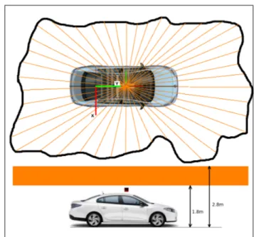
Extrinsic calibration of the sensor provides the position of the VLP-16 relative to the car frame. We convert each measurement from the sensor frame into the car frame by simple reference frame transformation (Eq. 1). The raw data provided by the VLP-16 corresponds to 3D measurements. Therefore, in order to obtain a planar scan information, we project the points belonging to the height range [1.8 m -2.8 m] on a horizontal plane (fig.3). The points chosen are higher than most cars and people, so in this step we remove from the system most of the perturbation due to moving objects, thus increasing the stability of the localization [1]. Moreover, the amount of information to be processed at each
iteration is drastically reduced when projecting from 3D to 2D laser scan, which allows the algorithm to run in real time on a conventional computer. Once the points are transformed into the car frame, the scan measurement can be addressed by an index in the vector of range measurements (Eqs. 2 and 3).
Fig. 3. Sensor configuration for Fluence. A 360◦ laser scan is obtained from the 3D point-cloud generated by the VLP-16. The bottom of the figure shows the point-cloud range involved in the generation of the planar scan.
The relation between the points in car and sensor frames is:
cP =cT
s∗sP (1) where sP is a point expressed in the sensor frame, cT
s is the constant transformation between the sensor frame and the car frame and cP = [x, y, z]T is point P expressed in the car frame. From these coordinates, we can extract the bearing angle α of P . Given the angular resolution of the scan, each value of α corresponds to a unique index in the output scan vector, given by equation 2.
i(α) = round( α
∆α) (2)
where ∆α is the angular resolution, in our case 0.5◦, and α ∈ [0, 360◦].
The range measured by the sensor for measurement index i is:
rangei= p
x2+ y2 (3) C. Ground truth generation
The ground truth position is computed using a Kalman filter that uses:
• The odometry pose. It is the result of integrating over time the speed of the car and its vertical angular velocity.
• The RTK-GPS position provided directly by the GPS receiver.
The GPS receiver provides localization at 1 Hz and the odometry is generated at 50 Hz, frequency of the speed measurements on the CAN bus of the car. The Kalman filter generates ground truth localization at the same frequency than the odometry (50 Hz). However, the RTK-GPS position is not always available, since it requires a minimum constel-lation of visible satellites and correct reception of corrections from the GPS ground station. In Section V, aerial views of the paths are provided. For each path, a color code reflects the precision of the GPS data, depending on the mode the system is in.
• GPS-Fix-RTK in green (+/-1 cm) • GPS-Float-RTK in blue (+/- 15cm) • GPS-Float in red (+/- 2-5m)
III. MAP BUILDING METHODOLOGY The localization method is based on a multi-map system that covers the length of the trip using 2D occupancy grid sub-maps. For building each of those sub-maps we apply 2D SLAM using ROS Gmapping [2] then each sub-map is geo-positioned using an optimization process that matches the local paths inside each sub-map with the global path obtained using the EKF GPS+odometry position. The reason why this method was chosen is because with respect to a local map the precision is quite acceptable for navigation, even though absolute precision might not be that good. On the other hand, the EKF GPS position can suffer from various disturbances, so its precision may locally be insufficient, while remaining globally consistent, meaning that it doesn’t diverge from the real position. This method takes advantage of both good qualities: good local sub-map precision and good global GPS consistency for positioning the sub-maps.
The sub-maps are positioned forming a chain in which two consecutive sub-maps are joined at common points called connection points. During the building phase, for each sub-map i we simultaneously record, at a predefined interval of distance Lthreshold, the path point in the map Pi
m = {Pjim}{j=0...Ni−1}, and the path point produced by
the EKF for the same instant. We also record the vari-ance of the localization error of the EKF solution Pi
g = {Pi
jg, σ
2
jg}{j=0...Ni−1}, where Ni is the number of points
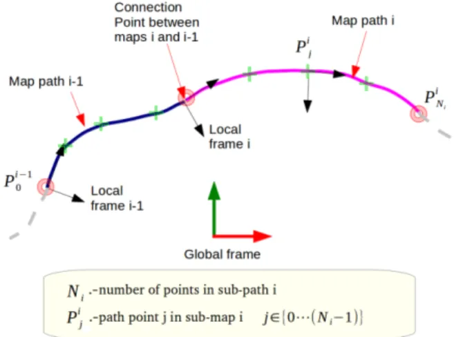
of the local path i. In this way we obtain two paths, the map path and the global path, produced respectively by the SLAM and EKF processes (See figure 4). The optimization by relaxation process for geo-positioning the maps is only applied when the sub-map under construction reaches a maximum size, so it takes little computing resources and can be run in real time on a standard computer.
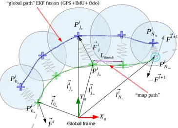
The points of both types of path are computed with respect to a common global reference system (see figure 5). The sub-maps are connected at the connection points to ensure continuity between them. We apply an iterative process of energy relaxation to fit the map and the global paths in such a way that the points that have a better EKF global precision intervene with higher weight than those with lower precision. The idea consists in considering the points of the global path like fixed points linked to the corresponding point in the map path by a virtual elastic force proportional
Fig. 4. Global path and Map path. Different sub-map paths are represented in different colors as a chain of sub-maps connected at the connection points. The green circles represent the localization error of the EKF solution.
Fig. 5. Global and local reference systems used in the optimization process.
to the distance between both points. The elasticity constant is defined as the inverse of the covariance of the global position error (figure 6). The output of the relaxation process is the sequence of sub-maps poses that produce a minimal energy, so the coherence of the information recorded on the global path and the map path are optimal. In practice, areas where the quality of the GPS is lower (for instance in urban canyons) or where it is inexistent (tunnels) produce global path points in which the uncertainty of the localization is high, so the corresponding forces with the respective map path point are weak or null. In this way, the method can cross areas of poor GPS coverage, provided they are not longer than the size of a sub-map, and yet ensure a good geo-positioning of the sub-maps.
IV. LOCALIZATION METHODOLOGY The localization uses a probabilistic process called Adap-tive Monte Carlo Localization (AMCL)[5], based on a par-ticle filter [4]. The main ideas of such an algorithm are:
• Each particle represents a likely position and orientation (posture) of the vehicle.
Fig. 6. Every point Pi
jpof the sub-map is attracted towards the
correspond-ing point Pjig with a force ~Fjiproportional to the inverse of the covariance of the position error covi
j and the relative position of the points ~lij. From
Newton’s action-reaction principle, at the connexion points Pi
Nmthe forces
between the sub-maps are opposed.
• The odometry equations are used to predict the posture of the particles at each iteration.
• Periodically, the filter calculates how well the LiDAR measurements fit the local sub-map, for each particle, with the result corresponding to the probability of the particle to hold the true posture of the vehicle. • Only the particles with a probability higher than a given
threshold survive, others are discarded.
• The particle with the highest probability is assumed to correspond to the current posture of the vehicle. • Whenever the number of remaining particles becomes
too low, a resampling around the last best fit is per-formed, in order to maintain a minimum number of particles.
In our extension of the algorithm, when the vehicle leaves a sub-map, a module called ”map manager” orders to load the next sub-map and initializes the local pose of the car on the new sub-map to ensure continuity of the localization process. As shown in figure 4, there is a certain amount of overlap between sub-maps, which guarantees the absence of ”gap” in the process.
V. EXPERIMENTAL CONDITIONS
Three scenarios have been considered for testing the localization system:
• Ring road of Nantes: little structured environment, higher speed and continuous traffic.
• Residential area: more structure than in the previous case, lower speed, and little traffic.
• Urban zone: structured zone like in the previous case, low speed and continuous presence of traffic in any direction.
Remarks about ring road scenario:
• On the ring road, the RTK coverage varies significantly from one test to another. In figure 7 a typical example is
Fig. 7. RTK-GPS coverage - Ring road of Nantes (RTK zones in green)
Fig. 8. RTK-GPS coverage - Residential zone (RTK zones in green)
shown. The total length in RTK mode is about 2.6 km. • In the chosen trajectory, the RTK-GPS coverage east of the river Erdre is, in general, quite bad. The precision of the localization in this part has essentially been evaluated on those short portions in which the GPS was in RTK mode. This is because there are multiple bridges crossing over the road that mask the signals coming from the satellites (red circles on the image of figure 7).
• In the part with good RTK coverage, the infrastructure is almost non existent, except the borders of the roadway. Remarks about residential scenario:
• The journey is located in the municipality of ”La Chapelle sur Erdre”, in the north of Nantes.
• The availability of RTK-GPS is quite repeatable from one test to another. Figure 8 shows a representative example.
• The RTK mode is available practically along the full trip. The total length in RTK mode is about 3.6 km. Remarks about the urban scenario:
• The journey is located in the north of Nantes.
• The availability of the RTK mode is globally good, but in the southern part it is less stable. Figure 9 shows a representative example. The total length in RTK mode is about 3.4 km.
Fig. 9. RTK-GPS coverage - Urban zone (RTK zones in green)
Fig. 10. Statistical summary for each scenario
VI. RESULTS AND ANALYSIS
Figure 10 shows a statistical summary of the results of the three scenarios. The minimum and maximum errors, the average error and its standard deviation over nine executions of the path are given.
Figure 11 shows the histograms of the lateral and longi-tudinal errors for each scenario and gives a visual idea of error distribution.
Figure 12 represents the series of standard deviations of the lateral and longitudinal errors for the individual experi-ments of each scenario. This figures shows in a visual way the repeatability of the experiments for the same trajectory by comparing the different individual tests.
The total distance analyzed along the ring road of Nantes is about 26 km, near 38 km in residential zone and about 34 km in urban zone. The experiments were conducted at different hours of the day, on different days. The total distance covered was about 100 km.
Here are a few observations we consider important: • The errors can be considered as centered.
Fig. 11. Lateral and longitudinal error histograms (ring road, residential, urban)
• The symmetry of the lateral error histograms is good, a little less for the longitudinal ones. In any case we cannot say there is any anomaly.
• The standard deviations are between 0.13 m and 0.22 m. As expected, the standard deviation of the error is higher on the ring road, with less structured environment than in the other two cases.
• Considering figures 10 and 12, we observe that the poorer quality of the localization on the ring road is duly reflected by the algorithm’s estimation of the standard deviation of the error.
• Figure 12 shows that the standard deviation obtained on different executions of a given scenario are repeatable. However, experiment number two (10 March 2017) shows a standard deviation of the error higher than the others. This particular experiment was conducted in foggy conditions. At this point, it would be premature to conclude that the fog is the cause of the result based on a single occurence of foggy conditions, but the matter certainly deserves further attention.
We have also noted that, in some of the experiments, there are rare situations where the error exceeds the ±3σ interval which, for a gaussian probability distribution, corresponds to an event of probability 0.27%. The standard deviation of the errors are produced by the AMCL algorithm, based on the dispersion of the particles and is just an approximation. Nev-ertheless, it fits quite well the real probability distribution, so it can be used as a quality estimator.
At this point one of the main questions that emerges is, which are the sources of error in the overall process? It would be difficult to enumerate all the error sources but we can at least mention the most important ones:
• Time stamping of the RTK-GPS measurements. The GPS measurements used in the experiments were time stamped with the time at which the NMEA message from the GPS reader arrives, minus a fixed delay that was estimated at 35 ms, which is approximately the time taken by the receiver to compute the position and send the result to the computer. Obviously, that is not optimal and should be computed dynamically by using techniques that uses the GPS PPS (Pulse Per Second) signal to obtain the correct time of measurement in computer’s time. The error introduced in the results by bad time stamping of the GPS measurements are related directly to the generation of the ground truth, not with the localization algorithm but, as we compare the ground truth and our localization, it affects the results. • Time stamping of the LiDAR data. The time stamp of the VLP-16 sensor is transfered to the planar 360◦scan, and this time stamp is of great importance when per-forming the ”update” phase in the particle filter. A delay in the laser time affects the SLAM process. As in the case of the RTK-GPS, the laser data was stamped with the time of arrival of the data. In order to be precise it should be stamped using the same PPS input as for the GPS.
• Noise in laser measurements. The laser sensor has an intrinsic measurements error of a few centimeters.
Additionally, the angular discretization of the scan pro-duces an uncertainty in the position of the measurement as well. These two effects combined cause the 3D measurement corresponding to a fixed point of the environment not to be totally static, specially if the vehicle moves.
• Projection of points from 3D to 2D. The fact that we project a range of height from the 3D cloud to a single 2D plane can also introduce some error, specially if the environment is not geometrically vertical, that is, for the same angle, all points in different heights do not project onto the same 2D position.
• Odometry error. Even though the odometry was care-fully calibrated, the short term prediction of the motion between two measurements is still affected by some noise.
VII. CONCLUSIONS AND FUTURE WORK Results of an intensive campaign of evaluation of a large scale mapping and localization experiment have been reported. The algorithms have proved to be very robust and their evaluation of the precision of the result reliable. Current accuracy may not yet be sufficient for autonomous navigation in the urban areas, but is getting close to the requirements. We feel that there is room for improvement of the performance with the same set of sensors, in particular through more precise data time stamping, which is the problem we wish to address in the near future.
ACKNOWLEDGMENTS
This work has been performed at the request of the French company Sherpa Engineering S.A. in April 2017. The LS2N is grateful to Sherpa for placing their trust in them and allowing the publication of the results of the study.
REFERENCES
[1] S. Nobili, S. Dominguez, G. Garcia, M. Philippe, “16 chan-nels Velodyne versus planar LiDARs based perception system for Large Scale 2D-SLAM,” in Proceeding in 7th Workshop on Plan-ning, Perception and Navigation for Intelligent Vehicles, PPNIV’15, IEEE/RS,September 28, 2015, pp. 131-136, Hamburg, Germany. [2] Grisetti, G. and Stachniss, C. and Burgard, W.,“Improved Techniques
for Grid Mapping With Rao-Blackwellized Particle Filters”, Robotics, IEEE Transactions on, February, 2007, pp. 34-46, ISSN 1552-3098. [3] S. Kohlbrecher, O. von Stryk, J. Meyer, and U. Klingauf, “A flexible
and scalable slam system with full 3d motion estimation,” in Safety, Security, and Rescue Robotics (SSRR), 2011 IEEE International Sym-posium on, Nov 2011, pp. 155–160.
[4] G. Grisetti and C. Stachniss and W. Burgard, “Improving Grid-based SLAM with Rao-Blackwellized Particle Filters by Adaptive Proposals and Selective Resampling”, in Proceedings of the 2005 IEEE International Conference on Robotics and Automation, April, 2005, pp. 2432-2437, ISSN 1050-4729.
[5] D. Fox , W. Burgard , F. Dellaert , S. Thrun ,“Monte Carlo Localiza-tion: Efficient Position Estimation for Mobile Robots”, in Proceedings of the National Conference on Artificial Intelligence, July, 1999, pp. 343-349, ISBN 0262511061.
[6] Hanten, Richard and Buck, Sebastian and Otte, Sebastian and Zell, Andreas, “Vector-AMCL: Vector based Adaptive Monte Carlo Lo-calization for Indoor Maps”, emphIntelligent Autonomous Systems (IAS), The 14th International Conference on, July, 2016, Shanghai. [7] S. Dominguez and B. Khomutenko and G. Garcia and P. Martinet,
“An Optimization Technique for Positioning Multiple Maps for Self-Driving Car’s Autonomous Navigation”, in 2015 IEEE 18th Interna-tional Conference on Intelligent Transportation Systems, September, 2015, pp.2694-2699, ISSN 2153-0009.