HAL Id: hal-00639040
https://hal.inria.fr/hal-00639040
Submitted on 8 Nov 2011
HAL is a multi-disciplinary open access
archive for the deposit and dissemination of
sci-entific research documents, whether they are
pub-lished or not. The documents may come from
teaching and research institutions in France or
abroad, or from public or private research centers.
L’archive ouverte pluridisciplinaire HAL, est
destinée au dépôt et à la diffusion de documents
scientifiques de niveau recherche, publiés ou non,
émanant des établissements d’enseignement et de
recherche français ou étrangers, des laboratoires
publics ou privés.
A 64 Kbytes ISL-TAGE branch predictor
André Seznec
To cite this version:
André Seznec. A 64 Kbytes ISL-TAGE branch predictor. JWAC-2: Championship Branch Prediction,
JILP, Jun 2011, San Jose, United States. �hal-00639040�
A 64 Kbytes ISL-TAGE branch predictor
∗
Andr´e Seznec
INRIA/IRISA
May 19, 2011
1
Outline
The ISL-TAGE predictor consists in a TAGE pre-dictor combined with a loop prepre-dictor (to predict loops) , a Statistical Corrector predictor and an Im-mediate Update Mimicker, IUM.
A TAGE predictor [4] constitutes the core of the ISL-TAGE predictor.
The TAGE predictor (Section 2) captures most of the correlation on the branch outcomes for very long histories. But sometimes TAGE fails to predict loops with constant number of iterations. The loop predic-tor (Section 3 ) is used to predict these loops. TAGE also fails to predict branches that are not strongly correlated, but only statistically biased. The Statis-tical Corrector predictor (Section 4) is in in charge of tracking these statistically correlated branches that are not correctly predicted by the TAGE predictor. The TAGE predictor must be updated at retire time to avoid pollution by the wrong path; this delayed up-date induces extra mispredictions compared with an optimistic at fetch time update. The Immediate Up-date Mimicker (Section 5) aims at limiting these ex-tra mispredictions through predicting branches with inflight non-retired occurrences.
The parameters of the submitted ISL-TAGE pre-dictor are summarized in Section 6 .
2
The TAGE conditional branch
pre-dictor
The TAGE predictor was described in [3] and [4]. Only marginal modification sare introduced here, es-sentially associated with the huge storage budget al-lowed for the contest.
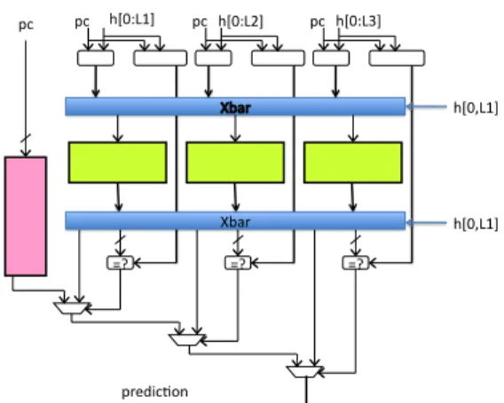
Figure 1 illustrates a TAGE predictor. The TAGE predictor features a base predictor T0 in charge of providing a basic prediction and a set of (partially) tagged predictor components Ti. These tagged pre-dictor components Ti, 1 ≤ i ≤ M are indexed using
∗This work was partially supported by the European Re-search Council Advanced Grant DAL
pc =? =? =? predic*on Xbar h[0:L1] pc pc h[0:L2] pc h[0:L3] h[0,L1] h[0,L1]
Figure 1: A 4-component TAGE predictor synopsis: a base predictor is backed with several tagged pre-dictor components indexed with increasing history lengths
different history lengths that form a geometric series [1], i.e, L(i) = (int)(αi−1∗ L(1) + 0.5).
Through-out this paper, the base predictor will be a simple PC-indexed 2-bit counter bimodal table; in order to save storage space, the hysteresis bit is shared among several counters as in [2].
An entry in a tagged component consists in a signed counter ctr which sign provides the predic-tion, a (partial) tag and an unsigned useful counter
u. Throughout this paper, u is a 1-bit counter and ctr is a 3-bit counter.
Sharing storage space between predictor ta-bles in the TAGE predictor The TAGE pre-dictor features independent logic tables. For some applications, some of the tables are underutilized while some others are under larger pressure. Shar-ing the storage space among several tables can be implemented without requiring to a real multiported memory table, but a bank interleaved tables as
illus-trated in Figure 1. Experiments showed that global interleaving of all tables is not the best solution, but that interleaving between for a few adjacent history lengths can be slightly beneficial (reduction of about 1% of the misprediction number on the distributed benchmark sets).
A few definitions and notations The provider
component is the matching component with the
longest history. The alternate prediction altpred is the prediction that would have occurred if there had been a miss on the provider component.
If there is no hitting component then altpred is the default prediction.
2.1
Prediction computation
The prediction selection algorithm is exactly the same in [3] or [4].
At prediction time, the base predictor and the tagged components are accessed simultaneously. The prediction is provided by the hitting tagged predictor component that uses the longest history. In case of no matching tagged predictor component, the default prediction is used.
However we remarked that when the confidence counter of the matching entry is null, on some traces, the alternate prediction altpred is sometimes more accurate than the ”normal” prediction. This prop-erty is global to the application and can be dy-namically monitored through a single 4-bit counter ( USE ALT ON NA in the simulator).
Prediction computation summary Therefore the prediction computation algorithm is as follows:
1. Find the longest matching component and the alternate component
2. if (the confidence counter is not weak or USE ALT ON NA is negative) then the provider component provides the prediction else the pre-diction is provided by the alternate component
2.2
Updating the TAGE predictor
Update on a correct prediction by the longest marching entry The prediction counter of the provider component is updated.
Update on a misprediction by the longest matching entry First we update the provider component prediction counter.
As a second step, if the provider component Ti is not the component using the longest history (i.e., i < M) , we try to allocate entries on predictor
components Tk using a longer history than Ti (i.e., i < k < M).
It should be noticed that, since, the predictor size storage budget allocated for the competition is huge we allocate up to 4 of these entries. For smaller pre-dictors, one would try to limit the footprint of the application on the predictor by allocating a single predictor entry. The M-i-1 uj useful bits are read
from predictor components Tj, i < j < M . The al-location algorithm chose up to four entries for which the useful bits are null, moreover we guarantee that the entries are not allocated in consecutive tables. When an entry is allocated, its prediction counter is set in weak mode and its useful bit is set to null. Updating the useful bitu The useful bit u of the provider component is set whenever the actual pre-diction is correct and the alternate prepre-diction altpred is incorrect.
In order to avoid the useful bits to stay forever set, we implement the following reset policy. On al-location of new entries, we dynamically monitor the number of successes and fails when trying to allo-cate new entries after a misprediction; this monitor-ing is performed through a smonitor-ingle 8-bit counter (u=1, increment, u=0 decrement). This counter (variable TICK in the simulator) saturates when more failures than successes are encountered on allocations. At that time we reset all the u bits of the predictor. Typically, such a global reset occurs when one of two entries on the used portion of the predictor has been set to useful. This simple policy was found to be more efficient than the previously proposed management using 2-bit useful counters for the TAGE predictor [4][3].
3
The loop predictor component
The loop predictor simply tries to identify regular loops with constant number of iterations.
The implemented loop predictor provides the global prediction when a loop has successively been executed 7 times with the same number of iterations. The loop predictor used in the submission features only 64 entries and is 4-way skewed associative.
Each entry consists of a past iteration count on 10 bits, a speculative and a retire iteration count on 10 bits each , a partial tag on 10 bits, a confidence counter on 3 bits, an age counter on 3 bits and 1 direction bit i.e. 47 bits per entry. The loop predictor storage is only 3,008 bits i.e. 376 bytes.
Replacement policy is based on the age. An entry can be replaced only if its age counter is null. On allocation, age is first set to 7. Age is decremented
whenever the entry was a possible replacement target and incremented when the entry is used and has pro-vided a valid prediction. Age is reset to zero whenever the branch is determined as not being a regular loop.
4
The Statistical Corrector Predictor
The TAGE predictor is very efficient at predict-ing very correlated branches even if the correlation is with very remote branches, e.g. on a 1000 bits branch history. However TAGE fails at predicting statistically biased branches e.g. branches that have only a very small bias towards a direction, but are not correlated to the history path. On some of these branches, the TAGE predictor performs worse than a simple PC-indexed table of wide counters.
In order to better predict this class of statistically biased branches, we introduce the Statistical Correc-tor predicCorrec-tor . The correction aims at detecting the unlikely predictions and to revert them: the predic-tion and the (address, history) pair is presented to Statistical Corrector predictor which decides whether or not inverting the prediction. Since in most cases the prediction provided by the TAGE predictor is cor-rect, the Statistical Corrector predictor can be quite small.
In the submission, the Statistical Corrector predic-tor is derived from the GEHL predicpredic-tor [1]. It fea-tures 5 logical tables indexed with the same history lengths as the main TAGE predictor (0, 3,8,12,17) and the prediction (taken/not taken) flowing out from the TAGE predictor. The logical tables are sharing a single interleaved 4K 6-bit entries, i.e., 3Kbytes. The prediction is computed as the sign of the sum of the (centered) predictions read on the Sta-tistical Corrector table plus the (centered) output of the hitting bank in TAGE (x8), thus taking into ac-count the confidence in the TAGE prediction. The TAGE prediction is reverted if the Statistical Cor-rector predictor disagrees and the absolute value of the sum is above a dynamic threshold. The dynamic threshold is adjusted at run-time in order to ensure that the use Statistical Corrector predictor is benefi-cial. The technique is similar to the technique used for dynamically adapting the update threshold of the GEHL predictor.
5
The Immediate Update Mimicker
On a real hardware processor, the predictor tables are updated at retire time to avoid pollution of the predictor by the wrong path. A single predictor table entry may provide several mispredictions in a row due to this late update. In order to reduce this impact, we
implement an add-on to TAGE, the IUM, immediate update mimicker.
However on a misprediction the history can be re-paired immediately and when a block is fetched on the correct path, the still speculative branch history is correct. In practice, repairing the global history is straightforward if one uses a circular buffer to imple-ment the global history. We leverage the same idea with IUM predictor. When fetching a conditional branch, IUM memorizes the identity of the entry E in the TAGE predictor (number of the table and its index) that provides the prediction as well as the pre-dicted direction. At branch resolution on a mispre-diction, the IUM is repaired through reinitializing its head pointer to the associated IUM entry and updat-ing this entry with the correct direction.
When fetching on the correct path, the associated IUM entry associated with an inflight branch B fea-tures the matching predictor entry E that provided the TAGE prediction and the effective outcome of branch B (corrected in case of a misprediction on B). In case of a new hit on entry E in the predictor be-fore the retirement of branch B, the (TAGE predictor + IUM) can respond with the direction provided by the IUM rather than with the TAGE prediction (on which entry E has not been updated).
IUM can be implemented in hardware through a fully-associative table, It allows to recover about 3/ 4th of the mispredictions due to late update of the TAGE predictor tables. The storage cost of the spec-ulative predictor is only 64*20 bits, i.e. 160 bytes, plus the pointers to determine the head ( position of the last fetch branch) and the tail ( position of the next to be retired branch) of the IUM.
Important remark : In the submission, the TAGE predictor, the Statistical Predictor and the loop predictor are re-read at retire stage to recom-pute the predictions, but also to get parameters such as the provider components etc before update. On a real hardware predictor, one would like to avoid this re-read and recomputation. The IUM could be aug-mented with a few fields (counter values, u bit, ..) to transmit these informations from fetch stage to re-tire stage, thus saving an extra read on the predictor tables.
6
The submitted ISL-TAGE predictor
6.1
The TAGE predictor component
For a 512 Kbits predictor, the best accuracy we found is achieved by a 16 components TAGE predic-tor, i.e. 15 tagged components and a base bimodalpredictor. Hysteresis bits are shared on the base pre-dictor. Each entry in predictor table Ti features a Wi bits wide tag, a 3-bit prediction counter and a 1-bit useful counter.
6.1.1 Tag width tradeoff
Using a large tag width leads to waste part of the storage while using a too small tag width leads to false tag match detections. Experiments showed that one can use narrower tags on the tables with smaller history lengths.
6.1.2 The global history vector
The usual combination of the global branch history vector and a short path history (limited to 1 bit per branch) was found to be slightly outperformed by a global history vector introducing much more infor-mation for the indirect branches as well as for the calls. 4 bits (resp. 5 bits) mixing target and program counter are introduced for the indirect branches and the calls.
6.2
TAGE parameters
Since this is competition we have run a guided search for the best set of history lengths. We first determined the number and respective sizes of tables in the predictor through exploring the design space using series of geometric history lengths. Then we grouped the tables to be interleaved. This leads to a configuration with 4 groups of tagged tables with increasing tag width, respectively T1-T2, T3-T7, T8-T13 and T14-T15. The set of possible history lengths was then explored with a geometric series with min-imum history length 8 and maxmin-imum history length 2000 as a starting point. The set of history lengths in the submitted predictor is {0, 3, 8, 12, 17, 33, 35, 67, 97, 138, 195, 330, 517, 1193, 1741, 1930}.
The characteristics of the TAGE component are summarized in Table 1. The base bimodal predictor features 32K prediction entries sharing 8K hysteresis entries. The TAGE predictor features a total of 482 Kbits of prediction storage.
Base T1-2 T3-7 T8-13 T14-15
Kentries 32+8 4 16 8 1
Tag bits 8 11 13 14
Kbits 40 48 240 136 18
Table 1: Characteristics of the TAGE predictor com-ponents
6.2.1 Total predictor storage budget
The total storage budget for the submitted ISL-TAGE predictor represents 61,696 bytes for ISL-TAGE predictor, 3,072 bytes for the Statistical Corrector predictor, 376 bytes for the loop predictor and 160 bytes for the IUM predictor, i.e a total of 65,304 bytes.
Apart the prediction tables storage, the ISL-TAGE predictor uses 1) a circular buffer to store the history, for convenience we use a a 4Kbits circular buffer, 2) two 12-bit pointers on the circular buffer, one for fetch history, the second for retire history 3) two 16 bits path history vectors 4) a 7-bit counter to determine the usefulness 5) a 8-bit counter to control the u bits reset 6) a 32-bit random number 7) two 6-bit point-ers on the IUM 8) two 6-bit countpoint-ers to manage the threshold on the statistical corrector, i.e. a total of 4,223 extra storage bits for control logic.
In total, the ISL predictor uses 65,833bytes of storage.
7
Options of the submitted
ISL-TAGE predictor
Through commenting some #define lines, one can run different versions of the submitted predictor.
#define IUM enables the IUM predictor. #define INITHISTLENGTH enables the use of the best found
set of history length. #define SHARINGTABLES enables the sharing of storage tables among the logic tables of the TAGE predictor. #define
LOOPPRE-DICTOR enables the loop predictor. #define STAT-COR enables the Statistical Corrector predictor.
References
[1] A. Seznec. Analysis of the o-gehl branch predic-tor. In Proceedings of the 32nd Annual
Inter-national Symposium on Computer Architecture,
june 2005.
[2] A. Seznec, S. Felix, V. Krishnan, and Y. Sazeid`es. Design tradeoffs for the ev8 branch predictor. In Proceedings of the 29th Annual International
Symposium on Computer Architecture, 2002.
[3] Andr´e Seznec. The l-tage branch predic-tor. Journal of Instruction Level Parallelism (http://wwwjilp.org/vol9), April 2007.
[4] Andr´e Seznec and Pierre Michaud. A case for (partially)-tagged geometric history length pre-dictors. Journal of Instruction Level Parallelism