HAL Id: hal-01387406
https://hal.inria.fr/hal-01387406
Submitted on 25 Oct 2016
HAL is a multi-disciplinary open access
archive for the deposit and dissemination of
sci-entific research documents, whether they are
pub-lished or not. The documents may come from
teaching and research institutions in France or
abroad, or from public or private research centers.
L’archive ouverte pluridisciplinaire HAL, est
destinée au dépôt et à la diffusion de documents
scientifiques de niveau recherche, publiés ou non,
émanant des établissements d’enseignement et de
recherche français ou étrangers, des laboratoires
publics ou privés.
Rare Events for Statistical Model Checking: An
Overview
Axel Legay, Sean Sedwards, Louis-Marie Traonouez
To cite this version:
Axel Legay, Sean Sedwards, Louis-Marie Traonouez. Rare Events for Statistical Model Checking: An
Overview. Reachability Problems, Sep 2016, Aalborg, Denmark. pp.23 - 35. �hal-01387406�
Rare events for Statistical Model Checking
An Overview
Axel Legay, Sean Sedwards and Louis-Marie Traonouez
Inria Rennes – Bretagne Atlantique
Abstract. This invited paper surveys several simulation-based approaches
to compute the probability of rare bugs in complex systems. The paper also describes how those techniques can be implemented in the profes-sional toolset Plasma.
1
Introduction
Model checking offers the possibility to automatically verify the correctness of complex systems or detect bugs [7]. In many practical applications it is also useful to quantify the probability of a property (e.g., system failure), so the concept of model checking has been extended to probabilistic systems [2]. This form is frequently referred to as numerical model checking.
To give results with certainty, numerical model checking algorithms effec-tively perform an exhaustive traversal of the states of the system. In most real applications, however, the state space is intractable, scaling exponentially with the number of independent state variables (the ‘state explosion problem’ [6]). Ab-straction and symmetry reduction may make certain classes of systems tractable, but these techniques are not generally applicable. This limitation has prompted the development of statistical model checking (SMC), which employs an ex-ecutable model of the system to estimate the probability of a property from simulations.
SMC is a Monte Carlo method which takes advantage of robust statistical techniques to bound the error of the estimated result (e.g., [22, 26]). To quantify a property it is necessary to observe the property, while increasing the number of observations generally increases the confidence of the estimate. Rare properties are often highly relevant to system performance (e.g., bugs and system failure are required to be rare) but pose a problem for statistical model checking because they are difficult to observe. Fortunately, rare event techniques such as
impor-tance sampling [17, 19] and imporimpor-tance splitting [18, 19, 24] may be successfully
applied to statistical model checking.
Importance sampling and importance splitting have been widely applied to specific simulation problems in science and engineering. Importance sampling works by estimating a result using weighted simulations and then compensating for the weights. Importance splitting works by reformulating the rare probability as a product of less rare probabilities conditioned on levels that must be achieved.
In this invited paper, we summarize our contributions on importance sam-pling and splitting. Then, we discuss their implementation within the Plasma toolset.
2
Command Based Importance Sampling
Importance sampling works by simulating a probabilistic system under a weighted (importance sampling) measure that makes a rare property more likely to be seen [16]. It then compensates the results by the weights, to estimate the probability under the original measure. When simulating Markov Chains, this compensation is typically performed on the fly with almost no additional overhead.
Given a set of finite traces ω∈ Ω and a function z : Ω → {0, 1} that returns 1 iff a trace satisfies some property, the importance sampling estimator is given by N ∑ i=1 z(ωi) df (ωi) df′(ωi) .
N is the number of simulation traces ωi generated under the importance
sam-pling measure f′, while f is the original measure. dfdf′ is the likelihood ratio.
For importance sampling to be effective it is necessary to define a “good” importance sampling distribution: (i ) the property of interest must be seen fre-quently in simulations and (ii ) the distribution of the simulation traces that satisfy the property in the importance sampling distribution must be as close as possible to the normalised distribution of the same traces in the original distribution. Failure to consider both (i ) and (ii ) can result in underestimated probability with overestimated confidence.
Since the main motivation of importance sampling is to reduce the compu-tational burden, the process of finding a good importance sampling distribution must maintain the scaling advantage of SMC and, in particular, should not iterate over all the states or transitions of the system. We therefore consider parametrised importance sampling distributions, where our parametrisation is over the syntax of stochastic guarded commands, a common low level modelling language of probabilistic systems1.
Each command has the form (guard, rate, action). The guard enables the command and is a predicate over the state variables of the model. The rate is a function from the state variables toR>0, defining the rate of an exponential
distribution. The action is an update function that modifies the state variables. In general, each command defines a set of semantically linked transitions in the resulting Markov chain.
The semantics of a stochastic guarded command is a Markov jump process. The semantics of a parallel composition of commands is a system of concurrent Markov jump processes. Sample execution traces can be generated by discrete-event simulation. In any state, zero or more commands may be enabled. If no
1
commands are enabled the system is in a halting state. In all other cases the enabled commands “compete” to execute their actions: sample times are drawn from the exponential distributions defined by their rates and the shortest time “wins”.
2.1 The Cross-Entropy Method
The “cross-entropy method” [25] is an optimisation technique based on minimis-ing the Kullback-Leibler divergence between a parametrised importance sam-pling distribution and the theoretically optimum distribution, without having an explicit description of the latter.
Given a system whose distribution is described by parametrised measure
f : Ω× Λ → R, where Λ is the set of possible vectors of parameters, using the
cross-entropy method it is possible to construct the following iterative process that converges to an estimate of λ∗, the optimal vector of parameters:
λ(j+1)= arg max λ N ∑ i=1 z(ωi(j))L(j)(ωi(j)) log df (ω(j)i , λ) (1)
N is the number of simulation runs generated on each of the j iterations, λ(j)
is the jth set of estimated parameters, L(j)(ω) = df (ω, µ)/df (ω, λ(j)) is the jth likelihood ratio (µ is the original vector of parameters), ω(j)
i is the ith path
generated using f (·, λ(j)) and df (ω(j)
i , λ) is the probability of path ω
(j)
i under
the distribution f (·, λ(j)).
2.2 Cross-Entropy Minimisation Algorithm
We consider a system of n stochastic guarded commands with vector of rate func-tions η = (η1, . . . , ηn) and corresponding vector of parameters λ = (λ1, . . . , λn).
In any given state xs, reached after s transitions, the probability that command
k∈ {1 . . . n} is chosen is given by
λkηk(xs)
⟨η(xs), λ⟩
,
where η is explicitly parametrised by xs to emphasise its state dependence and
the notation⟨·, ·⟩ denotes a scalar product. Let Uk(ω) be the number of
transi-tions of type k occurring in ω. We therefore have
df (ω, λ) = n ∏ k (λk)Uk(ω) ∏ s∈Jk(ω) ηk(xs) ⟨η(xs), λ⟩ .
We define ηk(i)(xs) and η(i)(xs) as the respective values of ηk and η functions
in state xsof the ith trace. We substitute the previous expressions in the
and li= L(j)(ωi) to get arg max λ N ∑ i=1 lizilog n ∏ k λui(k) k ∏ s∈Jk(i) ηk(i)(xs) ⟨η(i)(x s), λ⟩ = arg max λ N ∑ i=1 n ∑ k lizi ui(k) log(λk) + ∑ s∈Jk(i) log(ηk(i)(xs))− ∑ s∈Jk(i) log(⟨η(i)(xs), λ⟩) (2)
We denote the argument of the arg max in (2) as F (λ) and derive the following partial differential equation:
∂F ∂λk (λ) = 0⇔ N ∑ i=1 lizi ui(k) λk − |ωi| ∑ s=1 ηk(i)(xs) ⟨η(i)(x s), λ⟩ = 0 (3)
The quantity|ωi| is the length of path ωi.
Theorem 1 ([12]) A solution of (3) is almost surely a unique maximum, up to a normalising scalar.
The fact that there is a unique optimum makes it possible to use (3) to construct an iterative process that converges to λ∗:
λ(j+1)k = ∑N i=1liziui(k) ∑N i=1lizi ∑|ωi| s=1 η(i)k (xs) ⟨η(i)(xs),λ(j)⟩ . (4)
A rare property does not imply that good parameters are rare, hence (4) may be initialised by selecting vectors of parameters at random until one is found that allows some traces that satisfy the property to be observed. An alternative initialisation strategy is to simply choose the outgoing transition from every state uniformly at random from those that are enabled.
3
Importance Sampling For Timed Systems
The foregoing approach considers continuous time in the context of continuous time Markov chains (CTMC), where time delays in each state are sampled from exponential distributions. To reason on the stochastic performance of complex timed systems, the model of Stochastic Timed Automata (STA) [8] extends Timed Automata (TA) [1] with both exponential and continuous distributions. Work on closely related models [21] suggests that tractable analytical solutions exist only for special cases. Monte Carlo approaches provide an approximative alternative to analysis, but they incur the problem of rare events.
The added complexity of the STA model prevents a direct application of our approach for Markov chains, however in recent work we are applying im-portance sampling to STA by taking advantage of the symbolic data structures used to analyse TA. Our approach is to construct a simulation kernel based on a “zone graph” representation of an STA that excludes zones where the property fails. The probability corresponding to these “dead ends” is redistributed to the adjacent zones in proportion to the original probability of reaching them. The calculation is performed on the fly during simulation, by numerically solving an integral whose polynomial form is known a priori. All simulated traces reach goal states, while the change of measure is guaranteed by construction to reduce the variance of estimates with respect to the standard Monte Carlo estimator. Our early experimental results demonstrate substantial reductions of variance.
4
Importance Splitting
The earliest application of importance splitting is perhaps that of [17, 18], where it is used to calculate the probability that neutrons pass through certain shielding materials. This physical example provides a convenient analogy for the more general case. The system comprises a source of neutrons aimed at one side of a shield of thickness T . The distance traveled by a neutron in the shield defines a monotonic sequence of levels l0 = 0 < l1 < l2 < · · · < ln = T , such that
reaching a given level implies having reached all the lower levels. While the overall probability of passing through the shield is small, the probability of passing from one level to another can be made arbitrarily close to 1 by reducing the distance between levels. Denoting the abstract level of a neutron as l, the probability of a neutron reaching level lican be expressed as P(l≥ li) = P(l≥ li| l ≥ li−1)P(l≥
li−1). Defining γ = P(l≥ lm) and P(l≥ l0) = 1, we get
γ =
m
∏
i=1
P(l≥ li| l ≥ li−1). (5)
Each term of (5) is necessarily greater than or equal to γ, making their estimation easier.
The general procedure is as follows. At each level a number of simulations are generated, starting from a distribution of initial states that corresponds to reaching the current level. It starts by estimating P(l≥ l1|l ≥ l0), where the
dis-tribution of initial states for l0is usually given (often a single state). Simulations
are stopped as soon as they reach the next level; the final states becoming the empirical distribution of initial states for the next level. Simulations that do not reach the next level (or reach some other stopping criterion) are discarded. In general, P(l≥ li|l ≥ li−1) is estimated by the number of simulation traces that
reach li, divided by the total number of traces started from li−1. Simulations
that reached the next level are continued from where they stopped. To avoid a progressive reduction of the number of simulations, the generated distribution of initial states is sampled to provide additional initial states for new simulations, thus replacing those that were discarded.
4.1 Score function
The concept of levels can be generalised to arbitrary systems and properties in the context of SMC, treating l and liin (5) as values of a score function over the
model-property product automaton. Intuitively, a score function discriminates good paths from bad, assigning higher scores to paths that more nearly satisfy the overall property. Since the choice of levels is crucial to the effectiveness of importance splitting, various ways to construct score functions from a temporal logic property are proposed in [13].
Formally, given a set of finite trace prefixes ω ∈ Ω, an ideal score function
S : Ω → R has the characteristics S(ω) > S(ω′) ⇐⇒ P(|= φ | ω) > P(|= φ |
ω′), where P(|= φ | ω) is the probability of eventually satisfying φ given prefix
ω. Intuitively, ω has a higher score than ω′ iff there is more chance of satisfying
φ by continuing ω than by continuing ω′. The minimum requirement of a score function is S(ω)≥ sφ ⇐⇒ ω |= φ, where sφis an arbitrary value denoting that
φ is satisfied. Any trace that satisfies φ must have a score of at least sφand any
trace that does not satisfy φ must have a score less than sφ. In what follows we
assume that (5) refers to scores.
4.2 Fixed levels algorithm
The fixed level algorithm follows from the general procedure previously pre-sented. Its advantages are that it is simple,it has low computational overhead and the resulting estimate is unbiased. Its disadvantage is that the levels must often be guessed by trial and error – adding to the overall computational cost.
In Algorithm 1, ˜γ is an unbiased estimate (see, e.g., [9]). Furthermore, from
Proposition 3 in [4], we can deduce the following (1− α) confidence interval:
CI = [ ˆ γ/ ( 1 + z√ασ n ) , ˆγ/ ( 1−z√ασ n )] with σ2≥ m ∑ i=1 1− γi γi . (6)
Confidence is specified via zα, the 1− α/2 quantile of the standard normal
distribution, while n is the per-level simulation budget. We infer from (6) that for a given γ the confidence is maximised by making both the number of levels
m and the simulation budget n large, with all γi equal.
4.3 Adaptive levels algorithms
In general, however, score functions will not equally divide the conditional prob-abilities of the levels, as required by (6) to minimise variance. In the worst case, one or more of the conditional probabilities will be too low for the algorithm to pass between levels. Finding good or even reasonable levels by trial and er-ror may be computationally expensive and has prompted the development of adaptive algorithms that discover optimal levels on the fly [5, 13, 14]. Instead of pre-defining levels, the user specifies the proportion of simulations to retain af-ter each iaf-teration. This proportion generally defines all but the final conditional probability in (5).
Algorithm 1: Fixed levels
Let (τk)1≤k≤mbe the sequence of thresholds with τm= τφ
Let stop be a termination condition
∀j ∈ {1, . . . , n}, set prefix ˜ω1
j= ϵ (empty path)
for 1≤ k ≤ m do
∀j ∈ {1, . . . , n}, using prefix ˜ωk
j, generate path ωjkuntil (S(ωkj)≥ τk)∨ stop
Ik={∀j ∈ {1, . . . , n} : S(ωjk)≥ τk} ˜ γk= |Ink| ∀j ∈ Ik, ˜ωk+1j = ω k j ∀j /∈ Ik, let ˜ωjk+1be a copy of ω k
i with i∈ Ik chosen uniformly randomly
˜
γ =∏mk=1˜γk
Adaptive importance splitting algorithms first perform a number of simu-lations until the overall property is decided, storing the resulting traces of the model-property automaton. Each trace induces a sequence of scores and a corre-sponding maximum score. The algorithm finds a level that is less than or equal to the maximum score of the desired proportion of simulations to retain. The simulations whose maximum score is below this current level are discarded. New simulations to replace the discarded ones are initialised with states correspond-ing to the current level, chosen at random from the retained simulations. The new simulations are continued until the overall property is decided and the pro-cedure is repeated until a sufficient proportion of simulations satisfy the overall property.
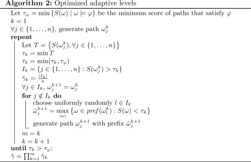
Algorithm 2 is an optimized adaptive algorithm that rejects a minimum number of simulations at each level (ideally 1, the one with a minimum score). This maximises the confidence for a given score function.
5
Plasma Lab Implementation
Plasma Lab [3] is a modular platform for statistical model-checking. The tool offers a series of SMC algorithms, included advanced techniques for rare events simulation, distributed SMC, non-determinism, and optimization. They are used with several modeling formalisms and simulators. The main difference between Plasma Lab and other SMC tools is that Plasma Lab proposes an API abstrac-tion of the concepts of stochastic model simulator, property checker (monitoring) and SMC algorithm. In other words, the tool has been designed to be capable of using external simulators, input languages, or SMC algorithms. This not only reduces the effort of integrating new algorithms, but also allows us to create direct plug-in interfaces with industry used specification tools. The latter being done without using extra compilers.
Plasma Lab architecture is illustrated by the graph in Fig.1. The core of Plasma Lab is a light-weight controller that manages the experiments and the distribution mechanism. It implements an API that allows to control the exper-iments either through user interfaces or through external tools. It loads three
Algorithm 2: Optimized adaptive levels
Let τφ= min{S(ω) | ω |= φ} be the minimum score of paths that satisfy φ
k = 1 ∀j ∈ {1, . . . , n}, generate path ωk j repeat Let T ={S(ωkj),∀j ∈ {1, . . . , n} } τk= min T τk= min(τk, τφ) Ik={j ∈ {1, . . . , n} : S(ωkj) > τk} ˜ γk= |Ink| ∀j ∈ Ik, ωk+1j = ω k j for j /∈ Ikdo
choose uniformly randomly l∈ Ik
˜ ωjk+1= max |ω| { ω∈ pref (ωk l) : S(ω) < τk } generate path ωk+1 j with prefix ˜ω k+1 j m = k k = k + 1 until τk> τφ; ˜ γ =∏mk=1˜γk Application-specific logics Application-specific
logics modeling languagesApplication-specific
Application-specific modeling languages SMC algorithms SMC algorithms Distribution and management Distribution and management
types of plugins: 1. algorithms, 2. checkers, and 3. simulators. These plugins com-municate with each other and with the controller through the API. The tool currently supports the following plugins for modeling language:
– Reactive Module Language (RML), the input language of the tool Prism for
Markov chains models.
– Biological language for writing chemical reactions.
– Simulink diagrams, using an interface to control the simulator of Matlab/Simulink – SystemC models, using an external tool to instrument SystemC models and
generate a C++ executable used by the plugin.
5.1 Importance sampling implementation
We have implemented importance sampling for the RML, allowing the user to specify sampling parameters that modify transition rates. These rates are au-tomatically used by Plasma Lab SMC algorithms to compute probabilities or rewards using the new sampling measure.
We have also implemented the cross-entropy minimization technique to iter-atively find an optimal parameters distribution. The initial parameters distribu-tion can be determined by selecting transidistribu-tions uniformly at random.
5.2 Importance splitting implementation
Importance splitting algorithms require the user to specify a score function over the model-property product automaton. This automaton is usually hidden in the implementation of the checker plugin. Therefore Plasma Lab includes a specific checker plugin for importance splitting that facilitates the construction of score functions. The plugin allows to write small observers automata to check proper-ties over traces and compute the score function. These observers are written with a syntax similar to the RML, using the notion of ‘guarded commands’ [10] with sequential semantics. This does not restrict the type of model being analyzed that can be different than RML.
These observers implement a subset of the BLTL logic presented in [15]. This subset ensures that the size of the property automaton does not depend on the bounds of temporal operators. As importance splitting algorithms require to restart simulations from random states (including the state of the property automaton), limiting the memory needed by this automaton facilitates the dis-tribution of the simulations over network computer grids. Finally the tool allows to translate BLTL properties from this subset into observers. The user needs only to edit the produced observers to compute an adequate score function for the property.
5.3 Distributed SMC algorithms
Simple Monte Carlo SMC may be efficiently distributed because once initialised, simulations are executed independently and the result is communicated at the
end with just a single bit of information (i.e., whether the property was satisfied or not). Importance sampling and the cross entropy algorithms can be distributed as easily.
By contrast, the simulations of importance splitting are dependent because scores generated during the course of each simulation must be processed cen-trally. The amount of central processing can be minimised by reducing the num-ber of levels, but this generally reduces the variance reduction performance. In [15] we propose a distributed fixed level importance splitting algorithm. It benefits from our welterweight observers to share states between the clients responsible for the simulations and the server responsible for dispatching the simulations. We also show that a distributed adaptive algorithms would be in-efficient because the number of levels is too high and consequently the number of simulations between each level is too low to benefit from the distribution.
Alternatively, entire instances of the importance splitting algorithms may be distributed and their estimates averaged, with each instance using a propor-tionally reduced simulation budget. This is the approach used in Plasma Lab to distribute importance splitting algorithms, but note that if the budget is reduced too far, the algorithm will fail to pass from one level to the next (because no trace achieves a high enough score) and no valid estimate will be produced.
5.4 Importance Sampling Results
Repair Model We first apply our cross-entropy minimisation algorithm to a repair
model from [23], using N = 10000 simulations per iteration. The system com-prises six types of subsystems containing (5, 4, 6, 3, 7, 5) components that may fail independently. The system’s evolution begins with no failures and with various probabilistic rates the components fail and are repaired. The respective failure and repair rates are (2.5ϵ, ϵ, 5ϵ, 3ϵ, ϵ, 5ϵ), ϵ = 0.001, and (1.0, 1.5, 1.0, 2.0, 1.0, 1.5). Each subsystem type is modelled by two guarded commands: one for failure and one for repair. The property under investigation is the probability of a complete failure of a subsystem (i.e., the failure of all components of one type), given an initial condition of no failures. This can be expressed in temporal logic as Pr[X(¬init Ufailure)].
Figure 2 plots the estimated probability and sample variance during the course of the algorithm, superimposed on a grey line denoting the true prob-ability calculated by PRISM. The long term average agrees well with the true value (an error of -1.7%, based on an average excluding the first two estimates). Without importance sampling we expect the variance of probability estimates of rare events to be approximately equal to the probability, hence Fig. 2 suggests that our importance sampling parameters provide a variance reduction of more than 105.
Chemical System We next consider a chemically reacting system of five molecular
correspond-0 5 10 15 20 Iteration 10 − 12 10 − 9 10 − 6 Probability Variance
Fig. 2. Repair model.
970 975 980 985 990 995 x Probability (i) (ii) 10 − 28 10 − 18 10 − 8 460 465 470 475 480 485 y
Fig. 3. Chemical system.
ingly named variables:
(A > 0∧ B > 0, A × B, A ← A − 1; B ← B − 1; C ← C + 1) (C > 0, C, C← C − 1; D ← D + 1) (D > 0, D, D← D − 1; E ← E + 1)
When simulated, A and B tend to combine rapidly to form C, which peaks before decaying slowly to D. The production of D also peaks, while E rises monotonically.
With an initial vector of values (1000, 1000, 0, 0, 0), we use N = 1000 simula-tions per iteration to estimate the probabilities of the following rare properties: (i ) F3000C ≥ x, x ∈ {970, 975, 980, 985, 990, 995} and (ii) F3000D ≥ y, y ∈ {460, 465, 470, 475, 480, 485}. We see from the results plotted in Fig. 3 that it is
possible to estimate extremely low probabilities with very few simulations. Note that although the model is intractable to numerical analysis, we have verified the estimates via independent simulation experiments.
5.5 Importance Splitting Results
We provide experimental results of two case-studies analysed with Plasma Lab importance splitting algorithms. For each model we performed a number of ex-periments to compare the performance of the fixed and adaptive importance splitting algorithms with and without distribution, using different simulation budgets and levels. Our results are illustrated in the form of empirical cumulative probability distributions of 100 estimates, noting that a perfect (zero variance) estimator distribution would be represented by a single step. The probabilities we estimate are all close to 10−6 and are marked on the figures with a verti-cal line. Since we are not able to use numeriverti-cal techniques to verti-calculate the true probabilities, we use the average of 200 low variance estimates as our best overall estimate.
As a reference, we applied the adaptive algorithm to each model using a single computational thread. We chose parameters to maximise the number of levels and thus minimise the variance for a given score function and budget. The resulting distributions, sampled at every tenth percentile, are plotted with circular markers in the figures. Over these points we superimpose the results of applying a single instance of the fixed level algorithm with just a few levels. We also superimpose the average estimates of five parallel threads running the fixed level algorithm, using the same levels.
Estimate × 107 Cum ulativ e probability 1 3 10 0 0.2 0.4 0.6 0.8 1 adaptive parallel fixed single fixed
Fig. 4. Leader election.
Estimate × 107 Cum ulativ e probability 5 10 20 40 0 0.2 0.4 0.6 0.8 1 adaptive parallel fixed single fixed
Fig. 5. Dining philosophers.
Leader Election Our leader election case study is based on the Prism model
of the synchronous leader election protocol of [11]. With N = 20 processes and
K = 6 probabilistic choices the model has approximately 1.2× 10¹⁸ states. We consider the probability of the property G420¬elected, where elected denotes the
state where a leader has been elected. Our chosen score function uses the time bound of the G operator to give nominal scores between 0 and 420. The model constrains these to only 20 actual levels (some scores are equivalent with respect to the model and property), but with evenly distributed probability. For the fixed level algorithm we use scores of 70, 140, 210, 280, 350 and 420.
Dining Philosophers Our dining philosophers case study extends the Prism
model of the fair probabilistic protocol of [20]. With 150 philosophers our model contains approximately 2.3× 10144 states. We consider the probability of the
property F30Phil eats, where Phil is the name of an arbitrary philosopher. The
adaptive algorithm uses the heuristic score function described in [14], which includes the five logical levels used by the fixed level algorithm. Between these levels the heuristic favours short paths, based on the assumption that as time runs out the property is less likely to be satisfied.
References
1. R. Alur and D. L. Dill. A theory of timed automata. Theor. Comput. Sci.,
126(2):183–235, 1994.
2. C. Baier and J.-P. Katoen. Principles of Model Checking (Representation and Mind
Series). The MIT Press, 2008.
3. B. Boyer, K. Corre, A. Legay, and S. Sedwards. PLASMA-lab: A flexible, dis-tributable statistical model checking library. In K. Joshi, M. Siegle, M. Stoelinga, and P. R. D’Argenio, editors, Quantitative Evaluation of Systems, volume 8054 of
LNCS, pages 160–164. Springer, 2013.
4. F. C´erou, P. Del Moral, T. Furon, and A. Guyader. Sequential Monte Carlo for rare event estimation. Statistics and Computing, 22:795–808, 2012.
5. F. C´erou and A. Guyader. Adaptive multilevel splitting for rare event analysis.
Stochastic Analysis and Applications, 25:417–443, 2007.
6. E. Clarke, E. A. Emerson, and J. Sifakis. Model checking: algorithmic verification and debugging. Commun. ACM, 52(11):74–84, Nov. 2009.
7. E. M. Clarke, Jr., O. Grumberg, and D. A. Peled. Model checking. MIT Press, Cambridge, MA, USA, 1999.
8. A. David, K. G. Larsen, A. Legay, M. Mikuˇcionis, D. B. Poulsen, J. V. Vliet, and Z. Wang. Statistical model checking for networks of priced timed automata. In
FORMATS, LNCS, pages 80–96. Springer, 2011.
9. P. Del Moral. Feynman-Kac Formulae: Genealogical and Interacting Particle
Sys-tems with Applications. Probability and Its Applications. Springer, 2004.
10. E. W. Dijkstra. Guarded commands, nondeterminacy and formal derivation of programs. Commun. ACM, 18(8):453–457, August 1975.
11. A. Itai and M. Rodeh. Symmetry breaking in distributed networks. Information
and Computation, 88(1):60–87, 1990.
12. C. Jegourel, A. Legay, and S. Sedwards. Cross-entropy optimisation of importance sampling parameters for statistical model checking. In P. Madhusudan and S. A. Seshia, editors, Computer Aided Verification, volume 7358 of LNCS, pages 327–342. Springer, 2012.
13. C. Jegourel, A. Legay, and S. Sedwards. Importance splitting for statistical model checking rare properties. In N. Sharygina and H. Veith, editors, Computer Aided
Verification, volume 8044 of LNCS, pages 576–591. Springer, 2013.
14. C. Jegourel, A. Legay, and S. Sedwards. An effective heuristic for adaptive im-portance splitting in statistical model checking. In Leveraging Applications of
For-mal Methods, Verification and Validation. Specialized Techniques and Applications,
pages 143–159. Springer, 2014.
15. C. Jegourel, A. Legay, S. Sedwards, and L.-M. Traonouez. Distributed verification of rare properties using importance splitting observers. ECEASST, 72, 2015. 16. H. Kahn. Stochastic (Monte Carlo) attenuation analysis. Technical Report P-88,
Rand Corporation, July 1949.
17. H. Kahn. Random sampling (Monte Carlo) techniques in neutron attenuation problems. Nucleonics, 6(5):27, 1950.
18. H. Kahn and T. E. Harris. Estimation of particle transmission by random sampling. In Applied Mathematics, volume 5 of series 12. National Bureau of Standards, 1951. 19. H. Kahn and A. W. Marshall. Methods of Reducing Sample Size in Monte Carlo
Computations. Operations Research, 1(5):263–278, November 1953.
20. D. Lehmann and M. O. Rabin. On the advantage of free choice: A symmetric and fully distributed solution to the dining philosophers problem. In Proc. 8thAnn. Symposium on Principles of Programming Languages, pages 133–138, 1981.
21. O. Maler, K. G. Larsen, and B. H. Krogh. On zone-based analysis of duration probabilistic automata. In 12th International Workshop on Verification of
Infinite-State Systems (INFINITY), pages 33–46, 2010.
22. M. Okamoto. Some inequalities relating to the partial sum of binomial probabili-ties. Annals of the Institute of Statistical Mathematics, 10:29–35, 1959.
23. A. Ridder. Importance sampling simulations of markovian reliability systems using cross-entropy. Annals of Operations Research, 134:119–136, 2005.
24. M. N. Rosenbluth and A. W. Rosenbluth. Monte Carlo Calculation of the Average Extension of Molecular Chains. Journal of Chemical Physics, 23(2), February 1955. 25. R. Rubinstein. The cross-entropy method for combinatorial and continuous opti-mization. In Methodology and Computing in Applied Probability, volume 1, pages 127–190. Kluwer Academic, 1999.
26. A. Wald. Sequential Tests of Statistical Hypotheses. The Annals of Mathematical