HAL Id: hal-00705289
https://hal.inria.fr/hal-00705289
Submitted on 7 Jun 2012
HAL is a multi-disciplinary open access
archive for the deposit and dissemination of
sci-entific research documents, whether they are
pub-lished or not. The documents may come from
teaching and research institutions in France or
abroad, or from public or private research centers.
L’archive ouverte pluridisciplinaire HAL, est
destinée au dépôt et à la diffusion de documents
scientifiques de niveau recherche, publiés ou non,
émanant des établissements d’enseignement et de
recherche français ou étrangers, des laboratoires
publics ou privés.
A Two-Phase Online Prediction Approach for Accurate
and Timely Adaptation Decision
Chen Wang, Jean-Louis Pazat
To cite this version:
Chen Wang, Jean-Louis Pazat. A Two-Phase Online Prediction Approach for Accurate and Timely
Adaptation Decision. International Conference on Service Computing, IEEE, Jun 2012, honolulu,
Hawaii, United States. �hal-00705289�
A Two-Phase Online Prediction Approach for
Accurate and Timely Adaptation Decision
Chen Wang and Jean-Louis Pazat
IRISA/INRIA, Campus de Beaulieu, 35042, Rennes Cedex, France Email:{chen.wang, jean-louis.pazat}@inria.fr
Abstract—A Service-Based Application (SBA) is built by defin-ing a workflow that composes and coordinates different Web services available via the Internet. In the context of on-demand SBA execution, suitable services are selected and integrated at runtime to meet different non-functional requirements (such as price and execution time). In such dynamic and distributed environment, an important issue is to guarantee the end-to-end Quality of Service (QoS). As a consequence, SBA provider is required to monitor each running SBA instance, analyze its runtime execution states, then identify proper adaptation plans if necessary, and finally apply the relative countermeasures. One of the main challenges is to accurately trigger the adaptation process as early as possible.
In this paper, we present a two-phase decision approach that can accurately analyze the adaptation needs for on-demand SBA execution model. Our approach is based on the online prediction techniques: an adaptation decision is determined by predicting an upcoming end-to-end QoS degradation through two-phase evaluations. Firstly, the end-to-end QoS is estimated at runtime based on monitoring techniques; if a QoS degradation is tent to happen, in the second phase, both static and adaptive strategies are introduced to assess whether it is the best timing to draw the final adaptation decision. Our approach is evaluated and validated by a series of realistic simulations.
Keywords-SBA; adaptation decision; SLA; quality prediction; classification;
I. INTRODUCTION
Service-Oriented Architecture (SOA) is adopted today by many enterprises as a flexible solution for building Service-Based Applications (SBA). An SBA is a dynamic and dis-tributed software system that integrates and coordinates a set of third-party Web services (named as the constituent services) accessible over the Internet. In this scenario, the SBA’s end-to-end Quality of Service (QoS) is determined by the QoS of all constituent services. For example, the execution time of an SBA instance depends on how fast each constituent service responds. However, in this loosely coupled environment, the execution of SBA may fail, or fail to meet the required quality level: a constituent service may take longer time to respond due to the network congestion; moreover, infrastructure fail-ures can cause a service completely responseless.
In this context, Service Level Agreement (SLA) plays an important role as a guarantee of non-functional quality. SLA is a mutually-agreed contract between service requester and provider, which dictates the expectations as well as obligations in regards to how a service is expected to be provided: on one hand, the expected quality level is formulated by specifying
agreed target values for a collection of QoS attributes; on the other hand, some penalty measures are defined in case of failing to meet these quality expectations. SLA violations can lead to some undesirable results, such as reputation degradation and penalty payment. To prevent SLA violation, it is essential for SBA providers to guarantee the end-to-end QoS by taking adaptation countermeasures if needed.
One of the key challenges is to determine the need for adaptation in order to draw accurate adaptation decisions. All existing approaches can be classified into two categories:
offline analysis[1], [2], [3] and online prediction [4], [5], [6]. Offline approaches can decide when and how to improve the end-to-end quality of SBA by reasoning the causes of the past SLA violations. The adaptation aims at preventing SLA violations for the future executions rather than the ongoing ones. By contrast, online approaches predict an upcoming SLA violation, and thereby decide to trigger preventive adaptation in order to improve the QoS of the running execution instance before the SLA violation really happens.
This paper investigates an online prediction approach for
on-demand executions of SBA. In this context, in response to different non-functional preferences and constraints (e.g. price and execution time), each constituent service is selected at runtime from a set of functional-equivalent candidates with different QoS [7]. As a result, any two distinct executions are instantiated with different configurations, defined as both local and global QoS expectations. Therefore, it is challenging to accurately predict potential SLA violations for all running SBA instances with irrelevant configurations.
In this paper, we introduce a two-phase online prediction approach to decide the best adaptation timing for on-demand executions of SBA. The first phase suspects an SLA violation by predicting an upcoming end-to-end QoS degradation; the prediction is based on the monitoring techniques and the estimation on the future execution. Later in the second phase, both static and adaptive strategies are introduced to predict the reliability of the suspicion in order to decide whether it is necessary to trigger preventive adaptations. Our approach is evaluated by a series of realistic simulations, the results show that our approach can determine both accurate and timely runtime adaptation decisions for on-demand SBA executions. The rest of paper is organized as follows: Section II provides the background of our problem. In Section III, some of the main existing decision approaches are discussed and our approach is introduced. Later, Section IV and Section V
Fig. 1. Illustrative Example: Travel Agency
present respectively the two phases of our approach in depth. In Section VI, the performance of our approach is studied based on a set of realistic simulations. Finally, the conclusion and the future work are addressed in Section VII.
II. BACKGROUND
A. Illustrative Example
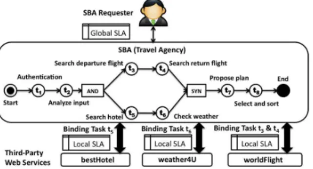
In this paper, we use a travel agency as an illustrative example to present our approach. As shown in Figure 1, an SBA is implemented to propose traveling plans for its clients. A request composes a set of parameters such as identifica-tion informaidentifica-tion (e.g. email address and password), dates of traveling and the destination. In order to respond to client’s requests, a workflow is defined to coordinate a collection of interrelated tasks: firstly, the client’s identity is verified by task t1and the inputs from the requester are validated and analyzed
by task t2. Then, the execution is diverged into two parallel
execution branches: taskt3and taskt4look for the round-trip
flight tickets from all airline companies. Concurrently, task t5 searches available hotels in the destination city, and the
weather information is provided by task t6. Both branches
converge before task t7, which generates all propositions of
traveling plans based on the client’s criterion, such as total budget. Finally, task t8 sorts all the propositions according to
the client’s preferences and returns the results.
The SBA requires service collaboration across enterprise boundaries: each task can be bound to either an internal service (e.g. taskt1, t2, t7, t8) or an external one provided by the
third-party enterprises (e.g. task t3, t4, t5, t6). Constituent services
are on demand selected at runtime: as an example, for premium clients, fast services are selected and bound in order to return the propositions of traveling plans as quickly as possible; on the other side, for normal clients, cheaper and slower services are used and the execution may take respectively longer time.
B. Global and Local SLA
As introduced, the SLA defines both aspects of expected QoS and penalty measures. First of all, the definition and execution of penalty is beyond the interests of this paper. Furthermore, we assume that a set of QoS attributes can be considered as deterministic: their values cannot be changed at runtime once negotiated (e.g. price). Accordingly, the SLA violation can be only caused by non-deterministic QoS at-tributes, whose real values are affected by the distributed and
TABLE I GLOBAL& LOCALSLAS
t1 t2 t3 t4 t5 t6 t7 t8 SBA
time (ms) 600 800 1500 1500 1800 1000 1200 1000 6800
Business Process
Monitor events Analyze decision Plan actions Execute apply message
Fig. 2. MAPE Control-Feedback Loop
dynamic runtime environment, such as response time. For the reason of simplicity, an SLA is therefore modeled as a set of target values for only non-deterministic QoS attributes. As a proof on concept, our discussion will only focus on the response time in the remainder of this paper.
The SBA plays the roles of service provider as well as consumer. For both roles, it negotiates an SLA with each of its counterparts, as shown in Figure 1: the SLA between the SBA and each constituent service is defined as local
SLA, and the one negotiated with the SBA requester is defined as global SLA. A local SLA reflects the expected time consumption for executing the corresponding task ti,
denoted as lsla(ti)=<qt(ti)>, whereas the global SLA dictates
the expected end-to-end execution time of SBA, denoted as
gsla=<gct>. Obviously, the definition of the global SLA
depends on the local ones. As an example, Table I lists the expected execution time defined in both global and local SLAs for an instance of the illustrative example shown in Figure 1.
C. Prevention of Global SLA Violation
In order to enhance the reputation and to avoid penalties, it is mandatory for service providers to prevent global SLA violation for every running execution instance. The general solution for runtime prevention of SLA violation is to im-plement the MAPE control-feedback loop (Monitor-Analyze-Plan-Execute) [8], as depicted in Figure 2: 1) Monitor: firstly, each execution instance of SBA is monitored by intercepting communication messages in order to collect a series of events; 2) Analyze: these events are used to evaluate the quality state of a running execution instance and to analyze the need for adaptation; 3) Plan: once an adaptation decision is determined, a suitable adaptation plan (e.g. a list of actions to improve the end-to-end quality) is identified; 4) Execute: finally the relative countermeasures are applied to the ongoing SBA instance.
D. Problem Definition
One of the key challenges to efficiently implement the MAPE loop is to accurately draw adaptation decision (Analyze step). Our research work studies an online prediction approach to analyze the need for adaptation by forecasting whether the SLA is tent to be violated in the future. An eligible online prediction approach has to meet the following require-ments (challenges): 1) Effectiveness. An effective approach can successfully predict as many SLA violations as possible. 2)
Precision. An effective approach might not be precise due to many false predictions, which will lead to unnecessary adaptations and thereby bring additional cost and complexity: on one hand, runtime adaptation is costly since more resources
are required to identify and to execute an adaptation plan; on the other hand, the time consumption of a runtime adaptation process may potentially delay the execution of SBA. 3) Timing. It is desirable to decide as early as possible: late decisions are usually precise but less useful, since the best adaptation opportunities might be missed, and the benefit of preventive adaptation is diminished. 4) Efficiency. The decision algorithm must be efficient (fast decision) in order to meet the critical time constraint at runtime.
III. RELATEDWORKANDMOTIVATION
A. Related Work
The existing online prediction approaches in the literature can forecast SLA violations caused by either functional
fail-ures or non-functional deviations. In the former case, the recovery from functional failures requires extra execution time and additional cost, which can lead to global SLA violations. Some research work use online testing techniques to test all constituent services in parallel to the execution of an SBA instance. By this means, an upcoming functional failure can be forecasted before its real occurrence. [9] presents the PROSA framework, which defines key activities to initiate online test-ing either on the bindtest-ing level or on the service composition level, and thereby proactively triggers the adaptation process. [10] investigates how to guarantee functional correctness of conversational services. The authors propose a novel approach to enables proactive adaptations through just-in-time testing. Online testing approach is helpful to detect potential functional failures but it can hardly be aware of the deviation of the end-to-end QoS. Furthermore, it requires each consistent service to provide a test mode (e.g. free interfaces for testing).
Our research work belongs to the latter case, which pre-dicts SLA violation by asserting non-functional deviations that might happen at the end of the execution (e.g. delay). Some research work use runtime verification techniques to determine the necessity of adaptation and to trigger preventive adaptation. In [6], the authors introduce SPADE approach: after the execution of each task, if the local SLA is violated, SPADE uses both monitored data and the assumptions to verify whether the global SLA can be still satisfied. If it reveals that the global SLA is tent to be violated, the adaptation is accordingly triggered. However, early verifications are largely based on the assumptions rather than monitored data, thus they are inaccurate and can lead to many unnecessary adaptations. Other research work use machine learning techniques in order to provide precise predictions and avoid unnecessary adaptations. In [4], a set of concrete points are defined in the workflow as checkpoints. Each checkpoint is associated with a predictor, which is implemented by a regression classifier. When the execution of the workflow reaches to a check-point, the corresponding predictor is activated and uses the knowledge learned from past executions to predict whether the global SLA will be violated. This work is extended in [5] by proposing the PREvent framework, which integrates event-based monitoring, runtime prediction of SLA violations and
Fig. 3. 2-Phase Online Prediction Approach
automated runtime adaptations. Such checkpoint-based predic-tion approach has some limitapredic-tions: firstly, some misbehavior (e.g. huge delay) between two checkpoints cannot be handled in time. In the meantime, the best adaptation opportunity might be lost. Furthermore, poorly selected checkpoint(s) may lead to undesirable results, such as unnecessary adaptations. But the selection of optimal checkpoints is complicated and challenging, especially for complex workflows.
B. Our Approach: Two-Phase Decision Approach
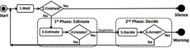
In order to provide both accurate and timely predictions of SLA violation, we propose a two-phase online prediction approach. As shown in Figure 3, an adaptation decision is determined through the following steps: 1) listen to the events emitted from the Monitor component (refer to Figure 2), once the execution of a task ti is completed, go to step 2. 2) If
the execution of workflow has not yet been finished, go to step 3; otherwise, the algorithm is terminated with the state
silence, which means that during the entire execution, no SLA violation has been predicted (no adaptation decision has been made). 3) Estimate the values of QoS attributes defined in the global SLA (e.g. execution time) based on the monitored data and the estimation of the execution in the future. 4) Compare the estimated value with the target value defined in the global SLA, if a violation is tent to happen, a suspicion of SLA violation is reported and go to step 5; otherwise, return to step 1. 5) Evaluate the trustworthy level of the suspicion in order to decide whether to accept or to neglect this suspicion. 6) If the suspicion is accepted, our approach terminates with the state warning by predicting an upcoming SLA violation and drawing the adaptation decision; otherwise, the suspicion is neglected and go back to step 1.
The core of our approach is two-phase evaluations: the
estimation phase (step 3, 4) evaluates whether the global SLA is tent to be violated and the decision phase (step 5, 6) evaluates how likely the suspected violation will really happen. An additional evaluation can bring more precise adaptation decisions since all inaccurate early suspicions can be neglected in the decision phase. Additionally, without the limitation of the predefined checkpoints, it is possible to react to any misbehavior in time. In the following, Section IV and Section V will use the execution time as an example to highlight respectively these two phases.
IV. ESTIMATIONPHASE
To estimate the end-to-end execution time of a running SBA instance, two kinds of information are required: 1) the measured execution time of the tasks whose executions have already been completed; 2) the probable time consumption of
uncompleted tasks, including the tasks that are being executed as well as the ones whose executions have not been started yet. Based on the monitoring techniques [5], we assume that the former information is known at the time of estimation, which is accessible from an internal database. In this section, we firstly highlight how to estimate local execution time for uncompleted tasks, and then we introduce an efficient tool for rapid estimation of the global execution time.
A. Estimation of Local Execution Time
The local execution time of a task ti depends on how fast
the corresponding constituent service SB(ti) responds. As a
result, some research work [5] propose to use arithmetic mean value of the last n measured response time of SB(ti) as the
estimation of the local execution time forti, denoted asqE(ti).
However, the performance of this method is affected by the outliers. Suppose that the last 10 measures of response time are: 940ms, 1,020ms, 1,050ms, 1,000ms, 970ms, 1,100ms, 1,020ms, 24,060ms, 960ms, 980ms. The arithmetic mean is 3,310ms, which cannot properly reflect the probable response time ofSB(ti). In addition, this method cannot be used when
there is no (sufficient) historical information. For example, in the context of on-demand SBA execution, a task may bind to a service that has never been invoked before.
We provide both dynamic and static methods for local esti-mation. To estimate the response time ofSB(ti), SBA provider
is required to record the response time of all constituent services that have been invoked before. Dynamic methods look into the past records for the information about SB(ti).
If enough historical information is found, the approaches presented in [11] can be used to firstly detect and remove the outliers before computing the arithmetic mean. A more efficient alternative solution is to directly use the median value of the last n measures. In the previous example, the median value is 1 000ms: five measures are less or equal to it and five are greater, including the outlier. In case of no (sufficient) historical information about SB(ti), the static
method is automatically activated, which uses the target value defined in the local SLA as the estimation (qE(ti) = qt(ti)).
In this case, it is straightforward to trust the service provider.
B. Estimation of Global Execution Time
Having the runtime knowledge on the local execution time of each task ti, defined as qL(ti), the global execution
time of a running SBA instance can be estimated by using aggregation functions [12] (qL(ti) equals to the measured
execution time for completed tasks and equals to qE(ti) for
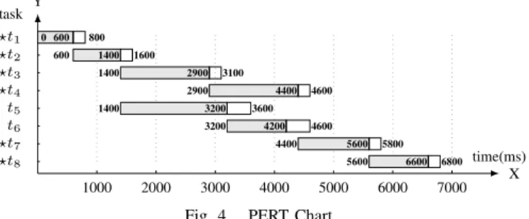
uncompleted ones). However, runtime aggregation is costly and time-consuming, especially for complex and unstructured workflows. We introduce the Program Evaluation and Review Technique (PERT) [13] as an efficient tool for rapid runtime estimation of global execution time. PERT was originally developed for planning, monitoring and managing the progress of complex projects. In our approach, PERT is used to manage the workflow execution and to facilitate decision making. It maintains some additional information for each task ti:
time(ms) X Y task 1000 2000 3000 4000 5000 6000 7000 ⋆t8 ⋆t7 t6 t5 ⋆t4 ⋆t3 ⋆t2 ⋆t1 0 600 800 600 1400 1600 1400 2900 3100 2900 4400 4600 1400 3200 3600 3200 4200 4600 4400 5600 5800 5600 6600 6800
Fig. 4. PERT Chart
• The Expected Start Time (EST): TE(ti). This is the
expected time by which the execution of tasktican start.
TE(ti) = max{TE(tj)+qL(tj)|tj is the direct precedent
of ti}, For the first task (start) ts,TE(ts) = 0.
• The Latest Finish Time (LFT):TL(ti). This is the latest
time by which the task ti can finish without causing
the delay of the ongoing execution instance. TL(ti) =
min{TL(tk) − qL(tk)|tk is the direct successor of ti}.
For the last task (end) tn, TE(tn) = gct, which is the
target value defined in the global SLA.
• The slack time: S(ti). This is the maximum delay for
executing the task ti.S(ti) = TL(ti) − TE(ti) − qL(ti). • The critical pathCP . A path is a sequential execution of
tasks from the beginning to the end of a workflow. CP is a path with all tasks having the least slack time. The PERT chart is initially constructed based on both global and local SLAs (qL(ti)=qt(ti)), all the information is then
presented on an X-Y chart. As an example, for the execution instance of the illustrative example with all local and global SLAs given in Table I, the corresponding PERT chart is computed and depicted in Figure 4. The X-axis represents the accumulated execution time, while the Y-axis is the list of tasks that are composed in the workflow. Each task ti is
represented by a single horizontal bar which starts fromTE(ti)
and ends withTL(ti). The length of the bar corresponds to the
maximum acceptable duration for executing a task, under the assumption that all the other tasks complete on schedule. A bar is composed of two parts, the solid part representsqL(ti)
and the hollow part reflects S(ti). Finally, the tasks on the
critical path is marked by a star (⋆).
In order to reflect the most up-to-date runtime execution state, the PERT chart can be updated when new local knowl-edge qL(ti) is available (e.g. newly measured execution time
of a just-completed task). Please note that the PERT chart only needs to be partially reconstructed by recomputing some of the above-mentioned information (e.g. the completed tasks do not need to be recomputed), which can be seen as the adjustments of some bars along the X-axis. The update can be triggered either periodically, or based on checkpoints or events (e.g. after each “invoke” event). Anyhow, the reconstruction of chart can be performed in parallel with the service invocations, thus it will not bring extra time consumption.
By using the PERT chart, the estimation of global execu-tion time is simplified. When a task ti is finished, the real
accumulated execution time at this moment can be measured, denoted as AT (ti). If AT (ti) > TL(ti), the global execution
time is estimated to be violated by AT (ti) − TL(ti), and a
global SLA violation is accordingly suspected. A suspicion of violation is represented by a pair, denoted as S=<TD, ti>,
which means that after executing task ti, a delay of TD is
estimated (TD=AT (ti)-TL(ti)). In this way, instead of running
complex aggregation function, the estimation of global SLA requires only one comparison operation.
V. DECISIONPHASE
In this section, both static and adaptive decision strategies are introduced to evaluate the trustworthy level of a suspicion in order to identify the need for the preventive adaptation.
A. Weight of a Suspicion
In the context of on-demand SBA execution, two suspicions with the same attributes (TD andti) reported by two distinct
SBA instances may have different significances. With different configurations, “after taskti” refers to the different degrees on
the completion of workflow execution. Using our illustrative example, S1 and S2 are both reported after task t7 with the
same estimated delay of 350ms; but forS1, 90% of the global
expected execution time (gct) is consumed after executingt7,
whereas only 60% for S2. Obviously,S1 is stronger thanS2
since a delay is more likely to happen in the end.
In order to model the significance of a suspicion S for on-demand executions of SBA, we introduce the concept of
weight, denoted as τs. τs is defined by a decimal between 0
and 1: greater value indicates a stronger suspicion. An earlier suspicion is often less accurate, because it is based more on the estimated values than on the measured values; accordingly it has a lower weight. Along with the execution, since more and more local estimations are updated with measured values, a later suspicion becomes more accurate and has a respectively higher weight. In our approach, the weight of a suspicion S is expressed by the percentage of execution that is supposed to be completed at the moment, defined as τs(S) = TL(ti)/gct,
remember that TL(ti) denotes the LFT of task ti and gct is
the expected global execution time defined in the global SLA. We provide three static strategies and an adaptive strategy to evaluate a suspicion S using the estimated delay TD and
its weight τs(S). Static strategies compute the maximum
allowed delay maxd with respect to τs(S) using predefined
evaluation functions. IfTDis greater thanmaxd, the suspicion
is considered as strong enough and an adaptation decision is determined; otherwise, it is neglected. By contrast, adaptive
strategy uses machine learning techniques to build a classifier that learns the knowledge from the past suspicions in order to predict whether or not the current suspicion will really happen.
B. Static Decision Strategies
1) Qualitative strategy: The idea is to neglect all the early suspicions since they are considered as inaccurate. By specifying a weight threshold ρw, only the suspicions with
τs > ρw will be accepted to report a warning of violation.
Thus, its evaluation function is a step function, as depicted by f1 in Figure 5:maxd equals to+∞ if τsis smaller than ρw
Fig. 5. Evaluation Functions of Static Decision Strategies and equals to 0 otherwise. Figure 5 also gives three sample suspicions with different weights and estimated delays: using qualitative strategy,S1will be neglected whereas bothS2and
S3 will be accepted.
2) Quantitative strategy: The main limitation of qualitative strategy is that the adaptation cannot be triggered until a certain percentage of workflow has been executed, despite the fact that a huge delay may arise at the beginning of the execution (e.g.S1). In order to react to such problem as early
as possible, quantitative strategy evaluates a suspicion with the consideration of bothτs(S) and TD. In this case, the SBA
provider specifies an evaluation function based on his/her own experience, such asf2 defined in Figure 5. Usingf2,S1 and
S2 will lead to adaptation decisions whileS3 will not.
3) Hybrid strategy: The quantitative strategy may not de-tect slight delays when the execution is approaching to the end, such asS3. In this case, a slight delay might finally lead
to a great penalty due to SLA violation. The hybrid strategy is more critical: by specifying ρw, if τs(S) is greater than
ρw, the qualitative strategy is applied (S will be absolutely
accepted); otherwise, the quantitative strategy is applied. Thus, its evaluation function follows f2 when τs< ρw and follows
f1 (maxd= 0) otherwise. By using hybrid strategy, all three
suspicions in Figure 5 will be accepted.
C. Adaptive Decision Strategy
Static decision strategies are useful when insufficient his-torical information is available. However, from the long-run perspective, it has the following limitations: first of all, it is a challenging task for the SBA provider to manually identify a suitable evaluation function based on his/her past experiences: sometimes such experience is hard to be expressed using a regular function. Additionally, once defined, the evaluation function cannot be self-adjusted (can be manually modified by SBA provider) in order to improve the quality of decision. The adaptive strategy models adaptation decision as a classification problem. The correctness of a suspicion (CS) can
be evaluated when the relative execution terminates (suppose no adaptation action is really executed): if the global SLA is really violated, the suspicion is proved as correct (CS=true);
otherwise, it is marked as a false one (CS=false). As a result,
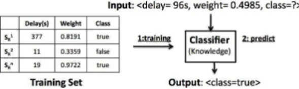
at the end of each execution, a set of suspicion records can be created based on all reported suspicions and their correctness. A suspicion record is described by two numeric attributes (estimated delay and its corresponding weight) and a categorical attribute defined as class (can be true or false),
Fig. 6. Adaptive Decision Strategy
denoted as SR=<TD, τs(S), CS>. All historical suspicion
records are organized into a training dataset, as illustrated in Figure 6. The dataset is often depicted as a table, with each row representing a suspicion record. Based on machine learning technique [14], a classifier is built to progressively learn the knowledge from past experiences. The knowledge is a specific algorithm that determines the class of a new suspicion based on its attributes. Once a suspicion is reported and it is classified as correct (CS=true), the adaptation decision is accordingly
made; otherwise, this suspicion is neglected.
Since the space is limited, we will not provide the details about data cleaning as well as how to learn and represent the knowledge. Interested readers can refer to [14], [15]. The classifier is required to be retrained to improve the prediction quality. The retraining can be carried out in one of the following ways: 1) after every N predictions, 2) periodically (after a fixed duration), 3) on-demand by the SBA provider.
VI. EXPERIMENTALRESULTS
A. Experiment Setup
Our approach is evaluated and validated by a set of ex-periments built on a realistic simulation model, since real implementation is costly, which requires to implement the entire MAPE control loop as well as dealing with some other challenging problems of on-demand SBA execution, such as service selection, or interface mismatches.
1) Realistic simulation model: For each constituent service, we are only interested in how it responds rather than what it responds. Therefore, instead of invoking real-world Web services, each task is bound to a virtual service, which only simulates the non-functional aspects of a service invocation (e.g. response time). In our experiments, 100 virtual services are created based on the realistic QoS datasets provided by [16], which record the non-functional performances (such as response time, throughput, etc.) of a large number of real-world service invocations. A virtual service collects all the invocation records from the same requester to the same Web service. By using these records, each virtual service defines two methods: 1) simulate() randomly selects one of the past records to simulate the non-functional aspects of an invocation; 2) getExpectedRT() determines the expected response time by specifying a percentage threshold φ, which indicates the percentage of past invocations which can respond within the expected value. In our experiments, in order to create a scenario with high violation rate,φ is set to 0.6 (40% possibility of local SLA violations for each virtual service).
2) Simulate an execution of SBA: An execution of SBA is simulated through three stages: in the first stage, an SBA instance is created by binding each task ti to a randomly
TABLE II CONTINGENCYTABLE
Real: violated Real: not violated Sum Prediction: violated True Positive (TP) False Positive (FP) Positive (warning) (correct warning) (false warning) (P) Prediction: not violated False Negative (FN) True Negative (TN) Negative (silence) (false silence) (correct silence) (N) Sum Violations (V) Compliance (C) Total (T)
selected virtual service, denoted as vs(ti), and the relative
local SLA is generated by completing a template with the expected response time of vs(ti). Then, the global SLA is
generated by computing the expected end-to-end execution time using aggregation functions [12]. Finally, based on both local and global SLAs, a PERT chart is constructed.
The second stage simulates the execution of this SBA instance. First of all, each selected virtual service vs(ti)
simulates the response time as the real execution time of task ti. Then, by running aggregation functions along all execution
paths, the real accumulated execution time by which the execution of taskti is completed can be computed, denoted as
AT (ti). Next, a collection of “receive” events are created with
the corresponding timestamp, denoted as Recv=<ti,AT (ti)>.
Finally in the third stage, these “receive” events are sorted by the timestamp and then sequentially processed: firstly, if AT (ti) > TL(ti), a set of predictors are activated to make
adaptation decision based on different strategies. A predictor is a Java object that implements a specific decision strategy. After the prediction, the PERT chart is updated and the static method is used for estimations of local execution time.
B. Evaluation Metrics
Contingency table metrics [17] are used to investigate how accurately a decision approach works. An adaptation decision approach can terminate with two possible states: warning or silence (refer to Figure 3). Using the contingency table, as shown in Table II, a warning is defined as a positive decision (P), which asserts that the global SLA will be violated in the near future; by contrast, a silence is formally named as a negative decision (N) which decides that no adaptation was needed for the entire duration of the execution. In order to evaluate the quality of decision, no adaptation plan is really identified and executed. For a positive decision, if a violation is really occurred in the end, it is proved to be a true positive (TP); otherwise, it is a false positive (FP). Similarly, a negative decision can be either a true negative (TN) if no violation really happens at the end of execution, or else a false negative (FN). Based on the contingency table, different evaluation metrics are defined as follows:
• Accuracy (a). It is the ratio of all correct decisions to the
number of all decisions: a = T P +T N +F P +F NT P +T N = T P +T NT .
• Precision (p). It is the ratio of all correct warnings to the
number of all warnings,p = T P T P +F P.
• Effectiveness (e). It is the ratio of all correct silences to
the number of all silences:e = T N T N +F N.
• Decision Time (dt). Only positive decisions have dt. It
is measured by the maximum number of tasks that have already been completed on different execution paths.
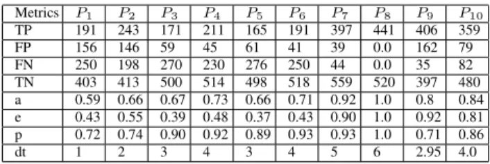
TABLE III
EXPERIMENTALRESULTS: EVALUATION OFDECISIONTIMING
Metrics P1 P2 P3 P4 P5 P6 P7 P8 P9 P10 TP 191 243 171 211 165 191 397 441 406 359 FP 156 146 59 45 61 41 39 0.0 162 79 FN 250 198 270 230 276 250 44 0.0 35 82 TN 403 413 500 514 498 518 559 520 397 480 a 0.59 0.66 0.67 0.73 0.66 0.71 0.92 1.0 0.8 0.84 e 0.43 0.55 0.39 0.48 0.37 0.43 0.90 1.0 0.92 0.81 p 0.72 0.74 0.90 0.92 0.89 0.93 0.93 1.0 0.71 0.86 dt 1 2 3 4 3 4 5 6 2.95 4.0
C. Experiment 1: Evaluation of the Best Decision Time
In this experiment, the best decision time is evaluated by disabling the decision phase, thereby the adaptation decision is determined once an SLA violation is suspected. The evaluation is based on the illustrative example defined in Figure 1: after each task ti (1 ≤ i ≤ 8), a checkpoint Ci is defined as a
possible decision time point. 8 predictors are created based on a single checkpoint: predictor Pi (1 ≤ i ≤ 8) can decide
only when the execution of workflow reaches to checkpoint Ci. Please note that the decisions of P8 must be definitely
accurate because it decides after the completion of workflow execution. In addition, two predictors are defined based on multiple checkpoints:P9 is activated at bothC2andC7while
P10 can decide at eitherC4 orC6. We run 1000 simulations,
Table III summarizes the performance of all predictors.
1) Decisions based on a single checkpoint: The results reveal that, by using a single checkpoint, it is hard to draw both early and accurate adaptation decision. First of all, as we discussed in this paper, early decisions are less accurate: due to the large number of FP and FN decisions, P1 andP2
result in lower accuracy, precision as well as effectiveness. By contrast, as the most part of workflow has been executed, P7
performs largely better but its decisions come too late to carry out effective preventive adaptations. Furthermore, the other four predictors are based on the checkpoints located on two parallel execution branches, and the critical path can be only determined at runtime due to on-demand service selection. If a task (checkpoint) is not on the critical path, it has thus a larger slack time and a longer delay can be tolerated. Therefore, from its local perspective, the execution is considered as running well and no warning will be reported. That explains why P3,
P4,P5andP6have less FP decisions but a tremendous number
of FN decisions, which lead to a poor performance on average.
2) Decisions based on multiple checkpoints: An additional checkpoint brings another chance to report (either true or false) warnings of SLA violations. Take P9 for example, if
a violation is failed to be predicted at C2, it still has chance
to be alerted at C7; thus, compared to P2, the TP number is
greatly improved; meanwhile, only several FP decisions are additionally produced. On the other side, compared toP7,
al-thoughP9does get some quality degradation, but the decision
time is improved by 2 execution steps. This is the same for P10, compared toP4 andP6, both accuracy and effectiveness
are significantly improved. However, as an extreme case, we assume that a predictor Px can draw adaptation decisions at
all possible checkpoints. It is similar to runtime verification
TABLE IV
EXPERIMENTALRESULTS: EVALUATEDIFFERENTDECISIONSTRATEGIES
Metrics P7 P9 P10 Pql Pqt Phb Pad
a 0.91 0.82 0.84 0.94 0.95 0.92 0.94 e 0.90 0.93 0.81 1.0 1.0 1.0 0.95 p 0.91 0.74 0.87 0.89 0.91 0.86 0.93 dt 5 3.04 4 4.2 3.9 3.8 3.8
techniques introduced in Section III: whenever a deviation is estimated, the adaptation decision is made. In this case, any a predictor fromP1toP8decides,Pxwill also decide. Thus,Px
cannot have less FP numbers thanP1. Such a high FP number
will result in a poor precision. From the above discussion, we can see that it is challenging to determine the best time for drawing both early and accurate adaptations decisions.
D. Experiment 2: Evaluation of Our Approaches
In the second experiment, both static and adaptive decision strategies presented in this paper are evaluated. The qualitative predictorPqlimplements qualitative strategy by specifying the
weight threshold ρw to 0.65. The quantitative predictor Pqt
defines the evaluation function asmaxd= (1 − τs)
3 2∗ gc
t∗ p,
where τs is the weight of a suspicion, gct is the expected
execution time of SBA defined in the global SLA, and p is set to 5%. This function can tolerate greater deviation at the beginning of the execution (as f2 in Figure 5). Additionally,
the hybrid predictor Phb invokes Pqt when the weight of
suspicion is less than 0.65, and usesPqlotherwise. Finally, the
adaptive predictor Pad implements a set of classifiers based
on WEKA machine learning toolkit [15]. All the decisions reported in the first experiment are used to generate a set of suspicion records, which are organized in the dataset file.
During the training phase (Step 1 in Figure 6), all classifiers are used to learn the knowledge from the dataset, and their performances are evaluated by cross-validation. When a new suspicion is reported, the classifier with the best predictive accuracy is then used for the prediction (Step 2 in Fig-ure 6). Each classifier requires at least 300 historical suspicion records (min training size=300); if the dataset contains more than 1000 records, it selects the 1000 most recent items (max training size=1000). The retraining is carried out for every 200 predictions.
Another 1000 executions are simulated to evaluate our approach. As a comparison, the three predictors with the best decision quality in the first experiment, namely P7, P9 and
P10, are also used. The performance of different predictors is
shown in Table IV. First of all, we can see that the quality of all static and adaptive decision strategies can be considered on the same level. Please note that: 1)Pqldecides later than the other
three strategies, since it can decide only when a certain part of workflow has been executed. 2) As introduced, Phb is more
critical than Pql and Pqt. Thus it accepts more suspicions,
which can result in a lower precision whereas a higher effec-tiveness. 3) Static strategies can successfully prevent almost all of SLA violations (luckily, in this experiment, no SLA violation has been missed). Meanwhile, adaptive strategy has a low rate of false silence (5%).
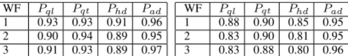
TABLE V ACCURACY WF Pql Pqt Phd Pad 1 0.93 0.93 0.91 0.96 2 0.90 0.94 0.89 0.95 3 0.91 0.93 0.89 0.97 TABLE VI PRECISION WF Pql Pqt Phd Pad 1 0.88 0.90 0.85 0.95 2 0.83 0.90 0.81 0.95 3 0.83 0.88 0.80 0.96 Secondly, compared to checkpoint-based predictors (single-step predictions), the results show that our approach can make more accurate adaptation decisions as early as possible. First of all, the decision quality of our approach can be considered on the same level as P7. But our approach improves the
decision time by more than one execution step. Secondly, P9 decides a little earlier than our approaches (less than one
execution step), but our approach has a remarkable improve-ment in accuracy (over 10%), effectiveness (5% higher on average) and precision (15% better). Finally, compare toP10,
our approaches have almost the same decision time but better accuracy (≈10%) as well as higher effectiveness (≈15%).
E. Experiment 3: Evaluations over Different Workflows
In order to evaluate the performance of our approach over different workflows, we create three fictitious workflows without real meanings: 1) a linear workflow with 9 tasks (a single execution path); 2) a medium workflow with 17 tasks and 6 execution paths; 3) a complex workflow with 30 tasks and 9 execution paths. For each workflow, we firstly simulate 300 executions to initiate the dataset of suspicion records, and then 1000 simulations are carried out by using Pql,Pqt,Phb
and Pad. Table V and Table VI summarize respectively the
accuracy and the precision of different predictors. From the experimental results, we have the following observations: 1) our approach is not limited to a specific workflow and it can perform well for different kinds of workflows; 2) adaptive strategy makes decisions based on the knowledge learned from the past executions, thus its performance can always be main-tained at a high level when used for different workflows; 3) the performances of static strategies depend on the predefined evaluation function: as the second experiment demonstrates, a suitable evaluation function can perform as well as adaptive strategy; otherwise, it may get a little performance degradation but it is still fairly good (compared to other approaches).
VII. CONCLUSION ANDFUTUREWORK
This paper discusses an important problem for preventing SLA violation: how to make correct runtime decision to accurately trigger preventive adaptation for on-demand SBA execution. In this paper, we have presented an online predic-tion approach which draws adaptapredic-tion decisions through two-phase evaluations. Based on a series of realistic simulations, our approach exhibits the following desirable properties: 1) it is able to draw accurate adaptation decisions for different workflows: almost all violations can be successfully predicted and alerted; meanwhile, only few unnecessary adaptations will be triggered; 2) with the same accuracy level, our approach can decide as early as possible; 3) by using static strategies, our approach can still make accurate and timely adaptation de-cision when no (sufficient) historical information is available.
Our future work will concentrate on providing more flexible runtime management of SBA. First of all, the PERT technique can be used for runtime optimization of SBA instances. For example, by using PERT charts, it is easy to detect large slack time for a task and thus it can rebind to a slower but cheaper service in order to reduce the cost. Furthermore, we are integrating branch prediction techniques into PERT charts, which can help to further reduce unnecessary adaptations. The re-construction of PERT chart will take into account the paths that are most likely to be executed. Finally, having positive results based on the realistic simulations, we are going to implement and integrate our approach into an existing business process management system and evaluate its performance.
ACKNOWLEDGMENT
The research leading to these results has received funding from the European Communitys Seventh Framework Pro-gramme [FP7/2007-2013] under grant agreement 215483 (S-CUBE).
REFERENCES
[1] L. Bodenstaff, A. Wombacher, M. Reichert, and M. Jaeger, “Monitoring dependencies for slas: The mode4sla approach,” in IEEE International Conference on Services Computing (SCC ’08), july 2008, pp. 21 –29. [2] ——, “Analyzing impact factors on composite services,” in IEEE
International Conference on Services Computing (SCC ’09), sept. 2009, pp. 218 –226.
[3] B. Wetzstein, P. Leitner, F. Rosenberg, I. Brandic, S. Dustdar, and F. Leymann, “Monitoring and analyzing influential factors of business process performance,” in 13th International Enterprise Distributed Ob-ject Computing Conference (EDOC ’09), 2009, pp. 141–150. [4] P. Leitner, B. Wetzstein, F. Rosenberg, A. Michlmayr, S. Dustdar, and
F. Leymann, “Runtime prediction of service level agreement violations for composite services,” in International Conference on Service-Oriented Computing (ICSOC/ServiceWave’09), 2009, pp. 176–186.
[5] P. Leitner, A. Michlmayr, F. Rosenberg, and S. Dustdar, “Monitoring, prediction and prevention of sla violations in composite services,” in IEEE International Conference on Web Services (ICWS’10), july 2010. [6] E. Schmieders and A. Metzger, “Preventing performance violations of service compositions using assumption-based run-time verification,” in 4th European Conference ServiceWave, 2011, pp. 194–205.
[7] L. Zeng, B. Benatallah, A. H.H. Ngu, M. Dumas, J. Kalagnanam, and H. Chang, “Qos-aware middleware for web services composition,” IEEE Trans. Softw. Eng., vol. 30, pp. 311–327, May 2004.
[8] J. Kephart and D. Chess, “The vision of autonomic computing,” Com-puter, vol. 36, no. 1, pp. 41 – 50, jan 2003.
[9] J. Hielscher, R. Kazhamiakin, A. Metzger, and M. Pistore, “A framework for proactive self-adaptation of service-based applications based on online testing,” in 1st European Conference ServiceWave, 2008. [10] D. Dranidis, A. Metzger, and D. Kourtesis, “Enabling proactive
adap-tation through just-in-time testing of conversational services,” in 3rd European Conference ServiceWave, 2010, pp. 63–75.
[11] V. Hodge and J. Austin, “A survey of outlier detection methodologies,” Artif. Intell. Rev., vol. 22, no. 2, pp. 85–126, Oct. 2004.
[12] M. Jaeger, G. Rojec-Goldmann, and G. Muhl, “Qos aggregation for web service composition using workflow patterns,” in 8th International Enterprise Distributed Object Computing Conference (EDOC), 2004. [13] D. L. Cook, Program Evaluation and Review Technique–Applications in
Education, 1966.
[14] M. Bramer, Principles of Data Mining. Springer, 2007.
[15] M. Hall, E. Frank, G. Holmes, B. Pfahringer, P. Reutemann, and I. H. Witten, “The weka data mining software: an update,” SIGKDD Explor. Newsl., 2009.
[16] Z. Zheng, Y. Zhang, and M. Lyu, “Distributed qos evaluation for real-world web services,” in 8th International Conference on Web Services (ICWS’10), july 2010, pp. 83 –90.
[17] F. Salfner, M. Lenk, and M. Malek, “A survey of online failure prediction methods,” ACM Comput. Surv., vol. 42, pp. 10:1–10:42, March 2010.