Université de Montréal
Le décodage des expressions faciales émotionnelles à travers différentes bandes de fréquences spatiales et ses interactions avec l’anxiété
par
Yann HAREL
Département de psychologie, Faculté des Arts et des Sciences
Mémoire
présenté en vue de l’obtention de la maîtrise (M.Sc.) en psychologie
sous la codirection de Franco Lepore et Fabien D’Hondt
1
Résumé
Le décodage des expressions faciales émotionnelles (EFE) est une fonction clé du système visuel humain puisqu’il est à la base de la communication non-verbale sur laquelle reposent les interactions sociales. De nombreuses études suggèrent un traitement différentiel des attributs diagnostiques du visage au sein des basses et des hautes fréquences spatiales (FS), respectivement sous-tendu par les voies magno- et parvocellulaires. En outre, des conditions telles que l’anxiété sociale sont susceptibles d’affecter ce traitement et d’entrainer une modulation des potentiels reliés aux évènements (PRE). Cette étude explore la possibilité de prédire le niveau d’anxiété social des individus à partir des corrélats électrophysiologiques du décodage d’EFE dans différentes bandes de FS. À cette fin, les PRE de 26 participants (âge moyen = 23.7 ± 4.7) ont été enregistrés lors de la présentation visuelle d’expressions neutres, de joie ou de colère filtrées pour ne retenir que les basses, moyennes ou hautes FS. L’anxiété sociale a été évaluée par l’administration préalable du questionnaire LSAS. Les latences et pics d’amplitude de la P100, N170, du complexe N2b/P3a et de la P3b ont été analysés statistiquement et utilisés pour entrainer différents algorithmes de classification. L’amplitude de la P100 était reliée au contenu en FS. La N170 a montré un effet des EFE. Le complexe N2b/P3a était plus ample pour les EFE et plus précoce pour les hautes FS. La P3b était moins ample pour les visages neutres, qui étaient aussi plus souvent omis. L’analyse discriminante linéaire a montré une précision de décodage d’en moyenne 56.11% au sein des attributs significatifs. La nature de ces attributs et leur sensibilité à l’anxiété sociale sera discutée.
Mots-clés : Expressions faciales émotionnelles, Fréquences spatiales, EEG, Potentiels reliés aux évènements, Anxiété sociale, Apprentissage machine, Analyse discriminante linéaire
2
Abstract
The decoding of emotional facial expressions (EFE) is a key function of the human visual system since it lays at the basis of non-verbal communication that allows social interactions. Numerous studies suggests that the processing of faces diagnostic features may take place differently for low and high spatial frequencies (SF), respectively in the magno- and parvocellular pathways. Moreover, conditions such as social anxiety are supposed to influence this processing and the associated event-related potentials (ERP). This study explores the feasibility of predicting social anxiety levels using electrophysiological correlates of EFE processing across various SF bands. To this end, ERP from 26 participants (mean age = 23.7 ± 4.7) years old were recorded during visual presentation of neutral, angry and happy facial expressions, filtered to retain only low, medium or high SF. Social anxiety was previously assessed using the LSAS questionnary. Peak latencies and amplitudes of the P100, N170, N2b/P3a complex and P3b components were statistically analyzed and used to feed supervised machine learning algorithms. P100 amplitude was linked to SF content. N170 was effected by EFE. N2b/P3a complex was larger for EFE and earlier for high SF. P3b was lower for neutral faces, which were also more often omitted. The linear discriminant analysis showed a decoding accuracy across significant features with a mean of 56.11%. The nature of these features and their sensitivity to social anxiety will be discussed.
Keywords: Emotional facial expressions, Spatial frequencies, EEG, Event-related potentials, Social anxiety, Machine learning, Linear discriminant analysis
3
Table des matières
Résumé………..3
Abstract……….4
Liste des figures………6
Liste des abréviations ………...7
Remerciements………..…8
Chapitre I : Introduction
Contexte théorique………10
Objectifs particuliers et hypothèses………...17
Contribution à l’article………...18
Chapitre II : L’article
The decoding of emotional facial expressions across various spatial
frequency bands and its interactions with social anxiety………20
Abstract……….21
Introduction………...22
Methods………...29
Results………...36
Discussion………...45
References………...51
Chapitre III : Discussion et conclusion
Discussion………...61
Conclusion………...65
4
Liste des figures
Figure 1 : Basic functioning of supervised machine learning algorithms.……..………27
Figure 2: Examples of filtered and normalized stimuli. …...…..……….31
Figure 3: Presentation of stimuli in an emotional oddball paradigm. Each stimulus is presented during 500 ms and followed by a fixation cross during 1300-1600 ms…………32
Figure 4: Example of stimuli constituting a single experimental block. ……..………..33
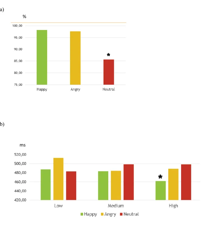
Figure 5: Behavioral data. a) The first graph shows mean precision, as % of correct detection. b) The second graph shows mean reaction times (ms)…….……….…44
Figure 6: Event-related potentials recorded at interest sites. Vertical axis is in µV, horizontal axis is in ms. The curves observed on Fz and Oz are difference waves obtained by subtracting the frequent stimuli from the rare ones. ……..………..……….39
Figure 7: Significant features for the four different classifiers and their corresponding decoding accuracies (DA). * indicates that the feature is significant at p<.05, ** indicates that the feature is significant at p<.01……..………..………..………..……44
5
Liste des abréviations
ADL (LDA): Analyse discriminante linéaire
EEG : Électroencéphalographie
EFE : Expression faciale émotionnelle
FFA : Fusiform facial area
FS : Fréquences spatiales
kNN : k-nearest neighbors
MEG : Magnétoencéphalographie
ms : Milliseconde
MVS (SVM): Machine à vecteur de support
PRE (ERP): Potentiels reliés aux évènements
6
Remerciements
Je souhaite en premier lieu remercier Franco Lepore, qui m’a ouvert sa porte et offert sa confiance avec tant de bienveillance que de générosité, ainsi que Fabien d’Hondt dont l’engagement inflexible et l’expertise infaillible m’ont été du plus grand secours.
Je ne peux pas non plus omettre de mentionner les membres du CERNEC au contact desquels je me suis constamment enrichi, Maria Van Der Knaap, Nathalie Bouloute, Stéphane Denis pour ne citer qu’eux, de même que les collègues Emma Campbell et Benjamin Hébert-Séropian, qui, non contents de m’avoir accepté dans un coin leur bureau m’ont aussi accepté dans un coin de leur cœur.
Mention spéciale à Antonin Tran, qui a su me faire profiter de l’arme de discussion massive la plus fertile qu’il m’ait été donné de rencontrer : son esprit.
Mention spéciale également à Charline Lavigne, qui, par sa curiosité, son intelligence et son entrain a permis de faire voler un projet qui battait de l’aile et que ma légèreté a bien failli plomber.
Je tiens aussi à remercier Karim Jerbi pour sa contribution aussi spontanée que providentielle, ainsi qu’Étienne Combrisson, pour sa patience et son travail qui ont adoucis mon atterrissage sur la surface dure et froide de l’apprentissage machine.
Enfin, ma gratitude éternelle se tourne vers mes parents, Patrice et Maicha, sans les bêtises desquels je ne serais littéralement pas là aujourd’hui mais qui eurent à cœur de se faire pardonner en m’offrant tout ce dont un fils peut rêver, incluant la formidable possibilité de poursuivre mes passions.
Je dédie ce mémoire à ma grand-mère, dont l’expression faciale de joie est à jamais gravée dans mes souvenirs et dont la présence paisible et sage m’a offert le meilleur remède possible contre l’anxiété.
7
8 Contexte théorique :
La capacité à décoder une expression faciale émotionnelle (EFE) joue un rôle crucial dans les interactions sociales chez l’humain, puisqu’elle permet une représentation rapide et efficace de l’état affectif d’autrui. Un nombre conséquent d’études indiquent que des dispositions stables de la personnalité telles que l’anxiété sociale peuvent moduler les premières étapes du traitement visuel des EFE (Staugaard, 2010). En outre, cette
modulation pourrait être reliée à une altération de l’usage des bandes de fréquences
spatiales (FS) chez les individus socialement anxieux (Lagner, Beck & Rinck, 2009). Cette étude vise à établir la faisabilité de prédire les niveaux d’anxiété sociale des individus via la modulation de l’activité cérébrale liée au traitement des EFE à travers différentes bandes de FS en utilisant la classification par apprentissage machine supervisé.
Potientiels reliés au décodage des visages. Parmi les nombreuses techniques utilisées pour étudier le décours temporel du traitement visuel des EFE avec
l’électroencéphalographie (EEG) ou la magnétoencéphalographie (MEG), la méthode des potentiels reliés aux évènements (PRE) est l’une des plus répandues, certainement grâce à sa résolution temporelle élevée, son ratio signal-sur-bruit important et ses coûts financiers faibles. Ces études rapportent que l’EFE et les propriétés psychophysiques du stimulus affectent différemment l’amplitude et/ou la latence des composantes de PRE
traditionnellement associées au traitement des visages. Les composantes précoces les plus étudiées sont la P100 (e.g., Ashley, Vuilleumier, & Swick, 2004; Batty & Taylor, 2003; Pizzagalli, Regard, & Lehmann, 1999; Pizzagalli et al., 2002) et la N170 (e.g., Batty & Taylor, 2003; Campanella, Quinet, Bruyer, Crommelinck, & Guerit, 2002; Righart & de Gelder, 2005; Stekelenburg & de Gelder, 2004). Plus tardivement, le complexe N2b/P3a et
9
la P3b permettent d’étudier le traitement des visages lors de stades décisionnels de plus haut niveau (Polich, 2007; Campanella et al., 2002).
P100. Dans ce contexte, l’influence de l’information affective sur les composantes liées au traitement des visages pourrait débuter dès la P100, tel que le suggèrent des études comparant le traitement d’expression émotionnelles (joie, colère, peur) avec des expression neutres (Pourtois et al., 2005; Kolassa & Miltner, 2006). La P100 est une déflexion
positive observée au niveau occipital environ 100 ms après l’apparition du stimulus, reflétant la réponse des cortex striés et extrastriés à une stimulation visuelle. Dans une expérience conduite par Vlamings, Goffaux & Kemner (2009), des expressions neutres et de peur ont été filtrées de manière à ne retenir que l’information de basses FS (BFS) ou de hautes FS (HFS). Lorsque ces stimuli étaient présentés dans une tâche de catégorisation, les expressions de peur évoquèrent une P100 d’amplitude plus large que les expressions neutres, et ce uniquement dans la condition de BFS. Cependant, ces résultats restent difficiles à interpréter à cause de la grande sensibilité de cette composante aux paramètres psychophysiques de bas-niveau (Rossion & Caharel, 2011) qui sont susceptibles de varier entre les expressions.
N170. La N170 est une composante négative apparaissant environ 170 ms post-stimulus visible sur les électrodes occipitotemporales. Considérée comme un indice de la finalisation du traitement configurationnel du visage (Schyns, Petro & Smith, 2007), la N170 est la composante la plus précoce à démontrer une amplitude plus élevée pour les visages que pour des objets (Bentin et al., 1996; Rossion, Curran & Gauthier, 2002). La N170 semble aussi varier en fonction de l’expression du visage présenté (Batty & Taylor, 2003, Blau et al., 2007), mais est relativement peu sensible aux paramètres
10
manipulés à travers les EFE (Eimer, 2011). De plus, certains auteurs ont observé une modulation de l’amplitude et de la latence de la N170 par le contenu émotionnel du visage uniquement en BFS, de manière semblable aux observations faites sur la P100 (Vlamings, Goffaux, & Kemner, 2009), tandis que d’autres ont observés une disparition de la N170 lorsque les stimuli étaient filtrés (Pourtois, Dan, Grandjean, Sander, & Vuilleumier, 2005).
N2b/P3a. Le complexe N2b/P3a est une composante attentionnelle impliquée dans la détection de la nouveauté et qui est traditionnellement observée sur la courbe de
différence obtenue par soustraction du stimulus fréquent (habitué) au stimulus rare. Il est communément observé entre 200 et 400 ms au niveau de l’axe médian fronto-pariétal, incluant une négativité pariétale (N2b) et une positivité frontale (P3a). L’information émotionnelle semble aussi avoir un effet sur l’allocation attentionnelle telle qu’indexée par le complexe N2b/P3a. Campanella et al. (2002) ont démontré à l’aide d’une tâche de oddball émotionnel consistant en une présentation sérielle de stimuli fréquents et rares que les latences de ce complexe étaient plus courtes lorsque les stimuli rares différaient du fréquent par l’émotion affichée, mais étaient retardées lorsque les stimuli rares et fréquents partageaient la même expression.
P3b. Finalement, la P3b est une large déflexion positive visible sur les électrodes centro-pariétales entre 300 et 600 ms, considérée comme reflétant une mise à jour de la mémoire de travail liée à la tâche (Polich, 2007). L’amplitude de cette composante a montré une modulation par la valence et l’activation émotionnelle des visages y compris lorsque ces dimensions n’étaient pas importantes pour la tâche, ce qui démontre la
sensibilité des étapes tardives du traitement visuel à l’information affective (Delplanque et al., 2004).
11
De nombreuses études investiguant les effets affectifs précoces sur le traitement des EFE ont aussi tenté de distinguer la contribution relative de l’information grossière (c.à.d. de BFS) et de l’information détaillée (c.à.d. de HFS). Cette approche fut encouragée par l’idée d’un traitement visuel par le cortex qui serait divisé en deux voies fonctionnellement distinctes : (1) la voie dorsale (occipito-pariétale), assurant un traitement visuo-spatial et (2) la voie ventrale (occipito-temporale) assurant la reconnaissance visuelle (Milner & Goodale, 2008; Ungerleider & Mishkin, 1982; voir aussi Kravitz, Saleem, Baker, & Mishkin, 2011 pour une revue récente). Cette ségrégation pourrait prendre son origine dès la rétine, puisque les bâtonnets sont connectés à la voie magnocellulaire qui projette de l’information de BFS à la voie dorsale, et les cônes sont connectés à la voie parvocellulaire qui projette de l’information de HFS à la voie ventrale (Baizer, Ungerleider, & Desimone, 1991; Bullier, 2001; Curcio, Sloan, Kalina, & Hendrickson, 1990; Merigan & Maunsell, 1993). Ainsi, un traitement affectif précoce des stimulations visuelles est susceptible de reposer sur une extraction rapide de l’information grossière par les aires du cortex visuel primaire qui pourraient interagir avec un « réseau affectif antérieur », constitué de structures sous-corticales telles que l’amygdale et le pulvinar, et de structures corticales telles que le pole temporal, le cortex insulaire et le cortex orbito-frontal (Barrett & Bar, 2009; Pessoa & Adolphs, 2010; Rudrauf, Mehta, Grabowski, 2008). Les PRE permettent donc d’étudier les étapes successives du traitement des visages, et leurs variations reflètent les modulations de ces étapes de traitement induites par la manipulation de paramètres faciaux véhiculant notamment l’information émotionnelle.
Modulation des PRE par l’anxiété. Étant donné l’importance des EFE pour les interactions sociales et leur capacité à déclencher des processus perceptifs et cognitifs, il n’est pas surprenant de remarquer que l’anxiété sociale semble moduler les PRE liés au traitement des visages (Staugaard, 2010; Rossignol et al., 2012a; Rossignol et al., 2012b).
12
L’anxiété sociale se caractérise par un biais négatif envers les attentes et perceptions sociales (Taddei, Bertoletti, Zanoni, & Battaglia, 2010). Cette disposition stable de la personnalité est ainsi liée à des biais dans la réactivité autonome aux stimuli émotionnels, l’allocation attentionnelle, la mémoire et la reconnaissance de même que dans des
processus cognitifs de plus haut niveau tels que les jugements subjectifs, les attentes et les interprétations de situations sociales (Staugaard, 2010). Lorsque ces processus sont étudiés à l’aide des PRE, des modulations de l’amplitude et de la latence des composantes par les niveaux d’anxiété sociale sont susceptibles d’apparaître lors des stades de traitement précoces et d’influencer par la suite les stades plus avancés. Par exemple, une étude
utilisant un paradigme de oddball émotionnel a démontré que des individus ayant un faible niveau d’anxiété sociale présentaient une P100 accrue en réponse à des visages de peur comparé aux autres stimuli émotionnels, tandis que les individus ayant un niveau élevé d’anxiété sociale présentaient une P100 accrue pour tous les stimuli émotionnels
(Rossignol et al., 2012a). Une autre étude utilisant une tâche d’indiçage spatial consistant à attirer l’attention du sujet dans une direction à l’aide d’un indice a mis en évidence une augmentation de l’amplitude de la P100 et de la P200 pour les individus ayant une anxiété sociale élevée, comparés avec des individus faiblement anxieux (Rossignol et al., 2012b). Van Peer et al., (2009) ont observé une augmentation de l’amplitude de la P150 en réponse aux EFE lorsque la réponse du participant est indiquée par l’évitement comparé à
l’approche d’un bouton de réponse après une administration de cortisol, et ce uniquement chez les patients ayant un haut niveau d’anxiété sociale. D’autres auteurs ont montré que la N170 obtenue par présentation de visages de colère était accrue chez les individus
socialement anxieux lorsque l’identification de l’émotion était utile à la tâche (Kolassa & Miltner, 2006). Étudiant des composantes plus tardives, Rossignol et al. (2007) n’ont pas trouvé de différences entre les groupes sur la P3b, mais les individus socialement anxieux
13
ont montré une N2b réduite pour les visages de colère comparés avec les visages de dégoût. Contrastant avec ces résultats, d’autres études ont montré une augmentation de l’amplitude de la P3 en réponse aux expressions menaçantes chez les individus atteints d’anxiété sociale (Moser et al., 2008) et une corrélation positive entre les scores d’anxiété sociale et l’amplitude de la P3 en réponse aux visages de colère. Finalement, une étude appliquant le paradigme des bulles (Gosselin & Schyns, 2001; Gosselin & Schyns, 2005) a montré lors d’une tâche de discrimination d’émotions que les individus ayant un niveau élevé d’anxiété social faisaient un plus grand usage de l’information de BFS que les sujets sains, tandis que les deux groupes avaient des performances similaires et faisaient un usage comparable des HFS au niveau des yeux (Langner, Becker & Rinck, 2009). L’étude des corrélats électrophysiologiques du traitement des visages représente ainsi un moyen de comprendre les mécanismes d’action de troubles mentaux tels que l’anxiété sociale. Dans cette étude, nous nous concentrerons sur les émotions de joie et de colère puisque celles-ci ont une valence opposée et qu’elles reflètent des émotions ayant une grande utilité sociale.
L’apprentissage machine comme méthode d’analyse des PRE. Diverses approt statistiques peuvent être utilisées afin de comparer les PRE, la plus courante étant l’analyse de variance (ANOVA; Luck, 2014). Néanmoins, cette méthode paramétrique possède plusieurs inconvénients tels que la nécessité d’assumer certains postulats qui sont rarement garantis pour des enregistrements électrophysiologiques. La classification par
apprentissage machine est une méthode statistique avancée qui a montré des résultats prometteurs dans la recherche des biomarqueurs de conditions pathologiques telles que la schizophrénie (Neuhaus et al., 2011; Neuhaus et al., 2013), le trouble déficitaire de l’attention (Mueller et al., 2010), la maladie d’Alzheimer, les troubles liés à la
consommation d’alcool, la dépression majeure et le trouble bipolaire par exemple (Orrù et al., 2012). Étant donné la taille importante et la haute dimensionnalité des ensembles de
14
données obtenues par les techniques d’imagerie cérébrale (incluant l’EEG et la MEG), cette approche possède l’avantage d’être guidé par les données et d’être en mesure de rechercher des relations entre un nombre important de variables, y compris dans les petits échantillons (Bishop, 2006). Une définition formelle de l’apprentissage machine a été donnée par Mitchell (1997) : « Un programme informatique apprend d’une expérience E en rapport à une tâche T et d’une mesure de performance P si sa performance à la tâche T, telle que mesurée par P, augmente avec l’expérience E » (Mitchell, 1997; traduction libre). Une forme particulière d’apprentissage machine, l’apprentissage supervisé, est
typiquement utilisé pour adresser les problèmes de classification puisqu’il permet
l’inférence d’une fonction de discrimination à partir de données préalablement labélisées
(Morhi, Rostamizadeh & Talwalkar, 2012). Lors d’une phase d’entrainement, des données
(ex. des enregistrements électrophysiologiques) ainsi que le label correspondant sont fournies à l’algorithme. Celui-ci est par la suite entrainé à trouver le meilleur moyen de prédire le label en utilisant les données fournies. Enfin, sa performance est testée en fournissant à l’algorithme un nouveau jeu de données sans le label correspondant, et le label prédit est comparé au label attendu afin d’établir la précision de la classification. Au cours des dernières décennies un certain nombre d’algorithmes ont été conçus afin de se comporter de cette manière, à savoir l’analyse discriminante linéaire (ADL), la machine à vecteur de support (MVS) et l’algorithme des k plus proches voisins.
L’ADL est un algorithme qui tente de trouver un hyperplan maximisant la distance moyenne entre deux classes tout en minimisant la variance interclasse (Fischer, 1936). L’ADL peut adresser un problème multi-classe en le réduisant à de multiples problèmes bi-classes et en discriminant chaque classe du reste en utilisant plusieurs hyperplans
(Fukunaga, 1990). Il est reconnu comme étant un algorithme rapide et direct, nécessitant d’assumer l’homoscédasticité des variables indépendantes (Combrisson & Jerbi, 2015). Le
15
principal inconvénient de cet algorithme est sa linéarité, qui peut être problématique pour des données non-linéaires complexes telles que les enregistrements EEG (Lotte et al., 2007).
La MVS recherche un hyperplan maximisant les marges entre l’hyperplan et les attributs les plus proches dans l’ensemble d’entrainement (Burges, 1998; Bennett &
Campbell, 2000; Vapnik, 1995). Pour les classes qui ne sont pas linéairement séparables, la MVS projette les attributs dans un espace de plus haute dimension en utilisant une fonction de noyau, réduisant ainsi le problème non-linéaire à un problème linéaire. Deux choix courants de noyaux sont la fonction de base radiale (FBR) et le noyau linéaire (Combrisson & Jerbi, 2015; Lotte et al., 2007; Thierry et al., 2016).
Enfin, l’algorithme des k plus proches voisins assigne à un nouveau point la classe dominante au sein de ses k plus proches voisins dans l’ensemble d’entrainement. Avec une valeur de k suffisamment élevée et assez d’échantillons d’entrainement, cet algorithme peut approximer n’importe quelle fonction ce qui lui permet de produire des frontières de décision non-linéaires. Lorsqu’utilisé dans des systèmes d’interface cerveau-machine avec des vecteurs d’attribut de basse dimension, cet algorithme montre une certaine efficacité (Borisoff et al., 2004).
Ainsi, par l’application de ces différents algorithmes d’apprentissage machine nous espérons clarifier la littérature existante sur les corrélats électrophysiologiques du
traitement des visages et leur modulation par l’anxiété sociale. Contrairement aux méthodes statistiques classiques, cette approche novatrice permet d’aborder la question sous un angle prédictif en utilisant les PRE pour déterminer le niveau d’anxiété sociale des participants. L’apprentissage machine pourrait ainsi permettre d’étendre notre
16
enfin, via son application aux interfaces cerveau-machine et aux dispositifs de neurofeedback, d’envisager de nouvelles approches thérapeutiques. Ces dernières
pourraient viser à renforcer ou diminuer l’activité cérébrale associée aux processus atteints par le trouble afin de pallier aux symptômes et d’enrayer sa progression.
Objectifs particuliers et hypothèses :
Dans la présente étude, cinq composantes de PRE liées au décodage de visages ont été extraites lors d’une tâche de oddball émotionnel, à savoir la P100, N170, N2b, P3a, et P3b. Les stimuli étaient préalablement filtrés afin de ne retenir que les basses, moyennes et hautes FS, et les visages affichaient une expression neutre, de joie ou de colère.
L’amplitude et la latence des composantes de PRE ont été utilisées pour entrainer les algorithmes d’apprentissage machine à prédire le niveau d’anxiété sociale des participants (bas, moyen, haut) tels que mesurés par la Liebowitz Social Anxiety Scale (LSAS). Au cours de la phase de test, la performance de classification (précision de décodage; PD) de chaque attribut et sa signification statistique ont été évaluées par validation croisée.
En dépit d’un nombre conséquent d’études investiguant les PRE liés au traitement des visages, cette expérience est la première à notre connaissance qui s’intéresse à
l’influence de différentes bandes de FS sur le décodage des EFE dans un contexte de
oddball émotionnel. Le but principal de cette étude est de déterminer la faisabilité d’utiliser
les PRE visuels classiques afin d’évaluer l’anxiété sociale à l’aide d’algorithmes
d’apprentissage machine supervisés. Nous émettons l’hypothèse que les attributs de BFS seraient de meilleurs prédicteurs des niveaux d’anxiété sociale que les attributs de MFS ou
17
HFS, et que les attributs obtenus avec les expressions émotionnelles seraient aussi de meilleurs prédicteurs que ceux obtenus avec les visages neutres. En outre, les objectifs complémentaires de cette étude sont (1) de déterminer l’effet de l’information affective sur les composantes précoces telles que la P100 et la N170, et si cet effet est dépendant du traitement des BFS, (2) d’évaluer le rôle de composantes attentionnelles plus tardives (le complexe N2b/P3a et la P3b) dans le décodage des EFE, et (3) de pointer la contribution relative des différentes bandes de FS à ce traitement.
Contribution à l’article :
Les hypothèses et le paradigme de cette présente étude furent élaborés par le Dr. Fabien D’Hondt, le Dr. Franco Lepore et Yann Harel. L’expérience a été programmée par Yann Harel, Fabien D’Hondt et Nathalie Bouloute. Le script exécutant le protocole expérimental a été développé par Yann Harel. Le traitement des images a été réalisé par Yann Harel. La collecte des données a été effectuée par Yann Harel, Charline Lavigne et Nathalie Bouloute. Les données ont été analysées par Yann Harel sous la supervision du Dr. Fabien D’Hondt. L’apprentissage machine a été réalisé par Yann Harel avec les outils informatiques créés par Étienne Combrisson et sous la supervision du Dr. Karim Jerbi. L’interprétation des résultats a été conduite par Yann Harel, sous la supervision du Dr. Fabien D’Hondt et du Dr. Karim Jerbi. Une première version de ce manuscrit, en cours de soumission pour publication, a été rédigée par Yann Harel et révisée par le Dr. Fabien D’Hondt et le Dr. Karim Jerbi.
18
19
The decoding of emotional facial expressions across various spatial frequency bands and its interactions with social anxiety.
Yann Harel12, Fabien D’Hondt23, Karim Jerbi124, Charline Lavigne12, Franco Lepore12
1Université de Montréal, Montréal, QC, Canada
2Centre de recherche en neuropsychologie et cognition (CERNEC) 3Université Lille Nord de France, Lille, France
20
Abstract
The decoding of emotional facial expressions (EFE) is a key function of the human visual system since it lays at the basis of non-verbal communication that allows social interactions. Numerous studies suggests that the processing of faces diagnostic features may take place differently for low and high spatial frequencies (SF), respectively in the magno- and parvocellular pathways. Moreover, conditions such as social anxiety are supposed to influence this processing and the associated event-related potentials (ERP). This study explores the feasibility of predicting social anxiety levels using electrophysiological correlates of EFE processing across various SF bands. To this end, ERP from 26 participants were recorded during visual presentation of neutral, angry and happy facial expressions, filtered to retain only low, medium or high SF. Peak latencies and amplitudes of the P100, N170, N2b/P3a complex and P3b components were statistically analyzed and used to feed supervised machine learning algorithms. P100 amplitude was linked to SF content. N170 was effected by EFE. N2b/P3a complex was larger for EFE and earlier for high SF. P3b was lower for neutral faces, which were also more often omitted. The linear discriminant analysis showed a decoding accuracy across significant features with a mean of 56.11%. The nature of these features and their sensitivity to social anxiety will be discussed.
21
Keywords: Emotional facial expressions, Spatial frequencies, EEG, Event-related potentials, Social anxiety, Machine learning, Linear discriminant analysis
1. Introduction
The ability to decode an emotional facial expression (EFE) plays a crucial role in human social interactions, for it allows for the fast and efficient representation of others affective state. There are substantial evidences that stable personality dispositions such as social anxiety could modulate early stages of the visual processing of EFE (Staugaard, 2010). Moreover, these modulations may be related to a differential use of spatial
frequency (SF) bands in socially anxious individuals (Langner, Beck & Rinck, 2009). This study aims to establish the feasibility of predicting social anxiety levels through the
modulation of brain activity linked to EFE processing across various SF bands using supervised machine learning classification.
On the many techniques that have been used to study the time course of EFEs visual processing with EEG or MEG, event-related potentials (ERP) is one of the most widely used, certainly due to its high temporal resolution, high signal-to-noise ratio and low financial costs. These studies report that EFE as well as psychophysical properties of the stimulus affects differently the amplitude and/or latency of ERP components related to face processing. Early components that are extensively studied includes the P100 (e.g., Ashley, Vuilleumier, & Swick, 2004; Batty & Taylor, 2003; Pizzagalli, Regard, & Lehmann, 1999; Pizzagalli et al., 2002) and N170 (e.g., Batty & Taylor, 2003; Campanella, Quinet, Bruyer,
22
Crommelinck, & Guerit, 2002; Righart & de Gelder, 2008; Stekelenburg & de Gelder, 2004). Later, the N2b/P3a complex and the P3b component also serves to study face processing at higher decisional stages. In this context, the influence of affective information on components linked to visual face processing may start as soon as the P100, as suggested by some studies comparing emotional expressions (happy, angry or fearful) to neutral expressions (Pourtois et al., 2005; Kolassa & Miltner, 2006). P100 is a positive deflection observed at occipital sites around 100 ms after the stimulus onset, and it is thought to reflect striate and extrastriate exogenous response to visual input. In an experiment conducted by Vlamings, Goffaux and Kemner (2009), neutral and fearful faces were filtered to retain either only low spatial frequencies (LSF) or high spatial frequencies (HSF). When these stimuli were presented in a categorization task, fearful faces evoked larger P100 amplitudes than neutral faces in LSF only. However, these results are hard to interpret due to the great sensitivity of P100 to low-level psychophysical parameters (Rossion & Caharel, 2011) that may vary between neutral and fearful expressions. N170 is a negative component that occurs at around 170 ms and is located at occipitotemporal electrodes. Considered to index configurational face processing (Schyns, Petro & Smith, 2007), the N170 is the earliest component to consistently show larger amplitude for faces than for non-faces (Bentin et al., 1996; Rossion, Curran & Gauthier, 2002). The N170 also seem to vary with emotional facial expression (Batty & Taylor, 2003, Blau et al., 2007), but is relatively insensitive to low-level psychophysical parameters such as contrast and luminance when these parameters are properly manipulated across EFE stimuli (Eimer, 2011). Moreover, some authors observed a modulation of N170 amplitudes and latencies by emotional content in LSF only, similar to those found on the P100 (Vlamings, Goffaux, & Kemner, 2009), and others didn’t observe any N170 at all when the stimuli were spatially filtered (Pourtois et al., 2005). The N2b/P3a complex is an attentional component specifically involved in novelty detection that is usually
23
observed on the difference waves obtained by subtracting the frequent (habituated) stimulus from the novel ones. It is commonly observed between 200 to 400 ms over the fronto-parietal midline with a parietal negativity (N2b) and a frontal positivity (P3a). Affective information also seem to have effects on attention allocation such as indexed by the N2b/P3a complex. Campanella et al. (2002) found in an oddball task that this complex’s latencies were shorter when the rare stimuli differed from the frequent by the displayed emotion, but were delayed when rare and frequent stimuli shared the same expression. Finally, P3b is a large positive deflection that takes place on centro-parietal sites between 300 to 600 ms, and is thought to reflect task-related memory updating (Polich, 2007). This components amplitudes have been found to be modulated by emotional arousal and valence of faces even when these dimensions were irrelevant to the task, thus indicating the sensitivity of latest processing stages to affective information (Delplanque et al., 2004).
Many studies that investigated early affective effects on EFE processing also tried to disentangle the relative contribution of coarse visual information (i.e. LSF) versus fine-grained, detailed information (i.e. HSF). This approach was encouraged by the view of cortical processing of visual inputs as subtended by two functionally distinct pathways: (1) the dorsal (occipito-parietal) stream ensuring visuo-spatial processing and (2) the ventral (occipito-temporal) stream allowing visual recognition (Milner & Goodale, 2008; Ungerleider & Mishkin, 1982; see also Kravitz, Saleem, Baker, & Mishkin, 2011 for a recent review). This segregation may originate from the retina since rod cells are linked to the magnocellular pathway which is thought to convey LSF information to the dorsal stream, and cones cells are linked to the parvocellular pathway which convey HSF information to the ventral stream (Baizer, Ungerleider, & Desimone, 1991; Bullier, 2001; Curcio, Sloan, Kalina, & Hendrickson, 1990; Merigan & Maunsell, 1993). Thus, an early affective processing of visual input may rely on the rapid extraction of coarse information by visual
24
cortical areas which could then interact with an “anterior affective network” constituted by subcortical structures such as the amygdala and pulvinar, and cortical structures such as the temporal pole, insular cortex and orbitofrontal cortex (Barrett & Bar, 2009; Pessoa & Adolphs, 2010; Rudrauf, Mehta, Grabowski, 2008).
Given the importance of EFE for social interaction and their potency to trigger perceptual and cognitive processes, it is unsurprising that social anxiety seem to modulate ERP linked to face processing (Staugaard, 2010; Rossignol et al., 2012a; Rossignol et al., 2012b). Social anxiety is characterized in social perceptions and expectations by a bias toward more negative social responses (Taddei, Bertoletti, Zanoni, & Battaglia, 2010). This stable disposition of personality is thus linked to bias in autonomic reactivity to emotional stimuli, attentional allocation, memory and recognition as well as in higher-level cognitive processes such as subjective ratings, expectancies and interpretations of social situations (Staugaard, 2010). When these processes are studied through ERP, modulations of components amplitudes and latencies by levels of social anxiety may arise at early stages and then influence more advanced processing stages. For example, a study using an emotional oddball paradigm found that low socially anxious individuals showed enhanced P100 in response to angry faces as compared to other stimuli, while high socially anxious participants displayed enlarged P100 for all emotional stimuli (Rossignol et al., 2012a). Another study using a spatial cueing task found enhanced P100 and P200 activity for high socially anxious participants as compared to low socially anxious (Rossignol et al., 2012b). Van Peer et al., (2009) observed an enhancement of P150 amplitudes to emotional faces during avoidance compared to approach after cortisol administration in patients with high social anxiety levels. Other authors found that the N170 response to angry faces was enhanced in socially anxious individuals when emotion identification was task-relevant (Kolassa & Miltner, 2006). Studying later components, Rossignol et al. (2007) didn’t find
25
any difference on P3b between groups, but high socially anxious individuals showed a reduced N2b activity for anger faces compared with disgust faces. Contrasting with these results, some other studies found an increase in P3 amplitude to threatening faces in high socially anxious individuals (Moser et al., 2008) and a correlation between social anxiety scores and P3 response to angry faces (Sewell et al., 2008). Finally, a study using the bubbles paradigm (Gosselin & Schyns, 2001; Gosselin & Schyns, 2004) showed in an emotion-discrimination task that high socially anxious individuals made greater use of LSF information than healthy controls, while both group had similar performances and made similar use of HSF around the eyes (Langner, Becker & Rinck, 2009).
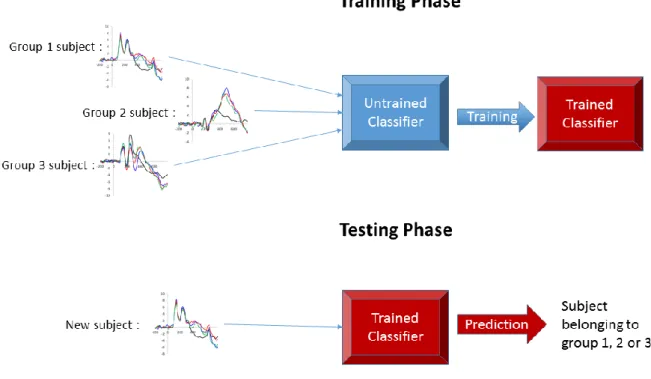
Machine learning classification is an advanced statistical method that showed promising results in the search for biomarkers of pathological conditions such as schizophrenia (Neuhaus et al., 2011; Neuhaus et al., 2013), ADHD (Mueller et al., 2010), Alzheimer’s disease, alcohol use disorder, major depression and bipolar disorder for example (Orrù et al., 2012). Given the large size and high dimensionality of datasets obtained with brain imaging techniques (including EEG and MEG), this approach possesses the advantages to be data-driven and to be able to look for relationships between a large number of variables even in small sample sizes (Bishop, 2006). A formal definition of machine learning was provided by Mitchell (1997) : "A computer program is said to learn from experience E with respect to some class of tasks T and performance measure P if its performance at tasks in T, as measured by P, improves with experience E". A specific form of machine learning, supervised learning, is typically used to address classification problems since it allows for the inference of a discrimination function from previously labeled data (Morhi, Rostamizadeh & Talwalkar, 2012). The basic functioning of such an algorithm is described in Figure 1 : During a training phase the algorithm is given data (eg. electro-physiological recordings) with the corresponding label. The algorithm will then train to find
26
the best way to predict the label according to the data that were given. Finally, its performance is tested by giving to the trained algorithm a new data sample without any labeling, and the label predicted by the algorithm is compared to the real label of these new data to determine the classification performance. Over the last decades, many algorithms were designed to behave in such a way, namely the linear discriminant analysis (LDA), the support vector machine (SVM) and the k-nearest neighbors (kNN) algorithms.
Figure 1 : Basic functioning of supervised machine learning algorithms.
LDA is an algorithm that tries to find a hyperplane that maximizes the mean distance between two classes while also minimizing the interclass variance (Fischer, 1936). LDA can address a multiclass problem by reducing it to multiple two-class problems and discriminating each class from the rest using multiples hyperplanes (Fukunaga, 1990). It is
27
recognized to be a fast and straightforward algorithm which needs to assume the homoscedasticity of independent variables (Combrisson & Jerbi, 2015). The main drawback of this algorithm is its linearity which may be problematic for complex nonlinear data such as EEG recordings (Lotte et al., 2007).
SVM searches for a hyperplane that maximize margins between the hyperplane and the closest features in the training set (Burges, 1998; Bennett & Campbell, 2000; Cortes & Vapnik, 1995). For classes that are non-linearly separable, SVM project features in a higher dimensional space using a kernel function, thus reducing the non-linear problem to a linear one. Two popular choices of kernel are the Radial Basis Function (RBF) and linear kernels (Combrisson & Jerbi, 2015; Lotte et al., 2007; Thierry et al., 2016).
Finally, the kNN algorithm assign to an unseen point the dominant class among its k nearest neighbors within the training set. With a sufficiently high value of k and enough training samples, kNN can approximate any function which enables it to produce nonlinear decision boundaries. When used in brain-computer interface systems with low-dimensional feature vectors, kNN may prove to be efficient (Borisoff et al., 2004).
In the present study, we extracted the five well-known ERP components linked to the visual processing of faces during an emotional oddball task, namely the P100, N170, N2b, P3a and P3b. Stimuli were previously filtered to retain only low, medium or high SF, and the target faces displayed either happiness, anger or a neutral expression. Amplitudes and latencies of these components were used to feed supervised machine learning algorithms that were trained to predict the social anxiety level (low, medium or high) of our participants, as assessed by the Liebowitz Social Anxiety Scale (LSAS). During the testing phase, the classification performance (decoding accuracy; DA) of each feature and its statistical significance were evaluated in a cross-validation framework.
28
Despite a consequent number of studies investigating ERPs linked to the visual processing of faces, this experiment is to our knowledge the first to look into the effects of spatial filtering on EFE processing in an oddball context. The primary goal of this study is to determine the feasibility of using classical visual ERPs in order to evaluate social anxiety in a sub-clinical sample through supervised machine learning algorithms. We hypothesize that LSF features would help predict social anxiety levels better than HSF or MSF features, and that features obtained with emotional faces would also be better predictors than those obtained with neutral faces. Moreover, complementary goals of this study are (1) to determine whether or not affective information have an effect on early components such as P100 and N170, and if this effect is dependent on the processing of LSF information (2) to evaluate the role of later attentional components (N2b/P3a complex and P3b) in the visual decoding of EFE, and (3) to shed light on the relative contribution of various spatial frequency bands to this processing.
2. Methods
2.1 Participants
Twenty-eight (16 females) right-handed participants (M=23.7 ±4.7 years old) were recruited at the University of Montreal through posters and announcements on social networks. The Beck Depression Inventory (Beck, Ward & Mendelson, 1961; BDI) and the Toronto Alexithymia Scale (Loas et al., 1996; TAS-20) were assessed online as screening measures respectively for depression and alexithymia. All the participants invited to take part in the experiment had a score of 20 or lower on BDI (which corresponds to categories less severe than Moderate Depression) and 50 or lower on TAS-20 (which corresponds to non-alexithymia). Before the experiment, participants also completed the State-Trait
29
Anxiety Inventory (Bruchon-Schweitzer & Paulhan, 1993; STAI), a scale divided into subscales measuring state anxiety and trait anxiety, for STAI-A and STAI-B respectively) and the Liebowitz Social Anxiety Scale (Liebowitz, 1987; LSAS M=25.31 ±15.691; STAI-A M=28.88 ±7.565; STSTAI-AI-B M=34.38 ±8.778). The three scales were highly correlated (LSAS and STAI-A : p=.019, ρ=.456; LSAS and STAI-B : p<.001, ρ=.708; STAI-A and STAI-B : p<.001, ρ=.725). In order to proceed to classification analysis, the participants were divided into 3 groups of nearly equal sizes on the basis of their LSAS scores. The LSAS scores were significantly lower for low socially anxious individuals (LSA; N=9, M=7.44 ±3.16) than medium socially anxious individuals (MSA; N=8, M=26.25 ±6.67), whom in turn scored lower than high socially anxious individuals (HSA; N=9, M=42.33 ±5.87; all p<.001).
2.2 Stimuli
The stimuli set was selected from the Radboud Face Database (Langner et al., 2010; RaFD) and comprised 24 grey pictures of eight individuals (four females), each posing neutrality, anger and happiness. The pictures were selected thanks to the validation study of RaFD according to three criteria: (1) each of them had an inter-judge agreement over 80% (mean = 95.71, SD = 5.21); (2) all neutral faces were judged as less intense (on a 5 points Likert scale from “weak” to “strong”) than emotional faces, F(2,21)=6.243, p=.007 (the difference was only significant for Happy compared to Neutral faces, p=.006; Angry versus Neutral, p=.286 ; Angry versus Happy, p=.265); and (3) the valence (from “negative” to “positive”) of angry faces was lower than neutral faces, which in turn was lower than happy faces, F(2,21)=299.867, p<.001 (all follow-up comparisons were significant at p<.001). Images were trimmed manually with Adobe InDesign (CC 2014). An ellipse of 275 by 413
30
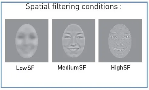
pixels containing only the facial features was extruded from each picture and placed at the center of a grey (red = 128, green = 128, blue = 128) square of 512 by 512 pixels. Invisible markers placed at 256 pixels (width) and 208 pixels (height) from the upper-left corner were used to manually adjust the position of the eyes and nose bridge. Based on previous literature (Goffaux et al., 2011) sets of second-order Butterworth filters were created with Matlab (R2014a) using the Image Processing Toolbox. Images were then filtered to retain only spatial frequencies between 2.48 and 9.58 cycles per face (cpf; 0.35 and 1.35 cycles per degree; Low spatial frequencies, LSF) when presented at a 57-cm distance, between 9.58 and 38.31 cpf (1.35 and 5.4 cpd; Medium spatial frequencies, MSF) or between 38.31 and 156.09 cpf (5.4 and 22 cpd; High spatial frequencies, HSF). Finally, the luminance and RMS contrast were normalized across all the created images using the SHINE Toolbox (Willenbockel et al., 2010; see Fig.2).
Figure 2: Examples of filtered and normalized stimuli.
31
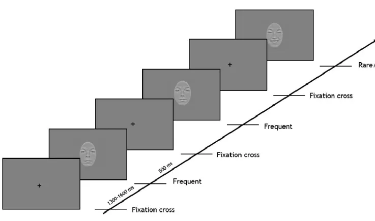
The participant sat in a dim light room, at a 57-cm distance from the computer screen. The task was to detect the occurrence of a rare stimulus in a sequence of frequent stimuli. Each stimulus was presented during 500 ms and followed by a black cross during an interval randomly varying between 1300 and 1600 ms (see Fig.3). The participant had 1500 ms after the stimulus onset to respond using the spacebar.
Figure 3: Presentation of stimuli in an emotional oddball paradigm. Each stimulus is presented during 500 ms and followed by a fixation cross during 1300-1600 ms.
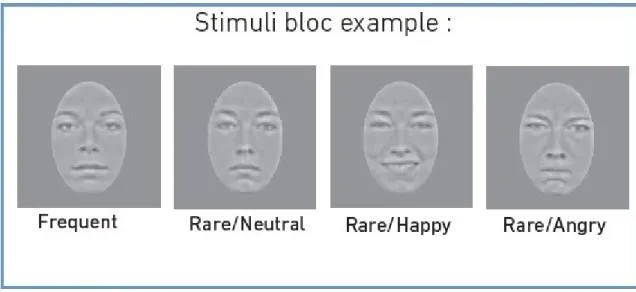
Eight blocks (75 trials per block) were constituted using the neutral face of a certain model as the frequent stimulus and the angry, happy and neutral faces of another model as the rare stimuli (6 occurrences each per block; see Fig.4). Those eight blocks were repeated for each filtering condition for a total of 24 blocks presented in a random order. After a series of 8 blocks, the participant took a 5 minutes break to relax.
32
Figure 4: Example of stimuli constituting a single experimental block.
2.4 ERP recording
Electroencephalogram (EEG) was recorded from the scalp using a 40 electrodes cap (10-20 system, Quick-Cap, NeuroMedical Supplies) connected to an amplifier (NuAmps, NeuroScan). The cap was placed on the subjects head using standard positioning references: nasion, inion and tragus. Four electrodes were used to record the electrooculogram for correction purposes (ocular movements and eye blinks). The impedance of all electrodes was maintained under 10kΩ, and the signal’s references were taken at both mastoids. The continuous EEG was recorded with a 1024 Hz sample rate and a band-pass filter of 0.1-300 Hz.
The EEG signal was then processed using EEGLab and ERPLab toolboxes for MatLab. The signals went through the PREP Pipeline in order to clean the data from non-biological noise and re-reference them to average after automatically excluding bad channels. An independent component analysis was then used to suppress ocular blinks from
33
all electrodes. An automatic artifacts rejection was performed to delete the signal contaminated by muscular artifacts. Two subjects were taken out of subsequent analysis because the automatic artifacts rejection left them with less than 70% of total trials. Epochs were created from 200 ms before stimulus onset to 800 ms after stimulus onset and a baseline correction was applied. Epochs were averaged for each condition and for each participant individually. A grand average of the ERP was explored visually in order to verify the presence and location of interest components, namely the P100, N170, N2b, P3a and P3b. Epochs were low-pass filtered at 30 Hz in order to make peak measures less sensitive to high frequency noise. Time windows and electrodes at which to measure peak amplitudes and latencies were selected for each component on the basis of previous literature and visual inspection of the grand average: P100 was observed between 120 and 160 ms at O1 and O2, N170 was observed between 160 and 220 ms at T5 and T6, and the P3b was observed between 300 and 600 ms at P3 and P4. The N2b/P3a complex was observed on the difference waves computed by subtracting the frequent stimulus from the rare stimuli. N2b was measured at Oz between 200 and 400 ms, and P3a was measured at Fz in the same temporal window.
2.5 Data analysis
2.5.1 General Linear Model
Analysis of variance (ANOVA) with repeated measures were conducted on mean response times and precision (percentage of detected rare stimuli) with Emotion (happy, angry, neutral) and Spatial frequency content (LSF, MSF, HSF) as the within-subject factors. The same factors were used for ANOVAs conducted on peak amplitudes and latencies, with the addition of the Hemisphere of recording (Left, Right) as a within-subject factor for the
34
P100, N170 and P3b components. The reported p-levels of all ANOVAs were corrected for violations of sphericity assumption when needed using the Greenhouse-Geisser epsilon correction. Simple effects were explored using t-tests with a Bonferroni correction for multiple comparisons. Only significant effects (level of significance at p=.05) are reported.
2.5.2 Data driven ERP analysis
Starting without any a priori assumptions about which ERP component may better predict social anxiety levels (namely LSA, MSA and HSA), P100, N170, N2b, P3a and P3b amplitudes and latencies measured at interest electrodes were analyzed in all target conditions. Data-driven analysis were carried out in Python 3.5, using Numpy and Scikit-Learn (Pedregosa et al., 2011) libraries.
We applied four widely used classification methods (Vapnik, 1998; Neuhaus et al., 2011): the linear discriminant analysis (LDA), the support vector machine (SVM) with two different kernels (radial basis function or linear), and the k-nearest neighbors algorithm (kNN) with k=5. The feature-selection method was based on cross-validation using the leave-one-subject-out strategy, thus training the algorithm on N-1 participants and testing the predicted class on the subject left out. Considering the fairly low number of subjects that were classified, the statistical significance of decoding accuracies was assessed through label permutation with a threshold of p=.05. Using the binomial cumulative distribution, the chance level of a 3-class problem on 26 participants was estimated at 50% (Combrisson & Jerbi, 2015).
35 3. Results
3.1 Behavioural data
Analysis on correct response latencies disclosed a Filter × Emotion interaction, F(4,100)=7.145, p<.001, η2=.222. This effect was broken down further by examining
Emotion separately for each filtering condition. An effect of Emotion was significant in HSF (F(2,50)=6.301, p=.016, η2=.201) : happy faces were detected faster than angry faces
(p<.001) and had a tendency to be also detected faster than neutral faces (uncorrected p=.026), although this effect wasn’t significant after Bonferroni correction (reducing the significance threshold at p=.017).
Analysis conducted on precision scores showed a main effect of Filter, F(2,50)=9.003, p<.001, η2=.265 : the stimuli in the MSF condition were more precisely
detected than in the LSF (p=.001) or HSF (p=.004) conditions. The analysis also detected a main effect of Emotion, F(2,50)=62.698, p<.001, η2=.715 : the Neutral face was less
precisely detected than the Happy and Angry faces (both p<.001). Finally, a significant Filter × Emotion (F(4,100)=5.033, p=.007, η2=.168) interaction was broken down by examining
the effect of Filter separately for each Emotion. The neutral face showed a significant effect of Filter (F(2,50)=8.194, p=.001, η2=.247) indicating that they were more precisely detected
36 a)
b)
Figure 5: Behavioral data. a) The first graph shows mean precision, as % of correct detection. b) The second graph shows mean reaction times (ms).
3.2 ERP results
3.2.1 P100 component at O1 and O2 (120-160 ms post-stimulus temporal windows) %
37
Amplitudes: A main effect of Filter, F(2,50)=45.267, p<.001, η2=.644 indicated higher
amplitudes for LSF, followed by MSF and then HSF (all p-values p<.001).
Latencies: The analysis didn’t detect any significant effect or interaction.
3.2.2 N170 component at T5 and T6 (160-220 ms post-stimulus temporal windows)
Amplitudes: First, a main effect of Hemisphere (F(1,25)=5.170, p=.032, η2=.171)
indicated that the amplitude was higher in the right hemisphere. Second, a main effect of Emotion (F(2,50)=19.653, p<.001, η2=.440) indicated that the amplitude was higher (more
negative) for the happy face than for the angry face (p=.027), which was in turn higher than for the neutral face (p=.004). Third, the analysis disclosed a significant Filter × Emotion interaction (F(4,100)=5.016, p=.001, η2=.167) that was broken down further by averaging
the Hemisphere and examining the effect of Filter separately for each Emotion. A significant effect of Filter (F(2,50)=8.857, p=.002, η2=.262) on happy faces indicated that the amplitude
was lower in the MSF than in the LSF (p=.004) and HSF (p<.001) conditions.
Latencies: A main effect of Emotion (F(2,50)=8.875, p=.001, η2=.262) indicated
earlier latency for the neutral face as compared to angry (p=.006) and happy (p=.003) faces.
3.2.3 N2b component at Oz (200-400 ms post-stimulus temporal windows)
Amplitudes: A main effect of Emotion, F(2,50)=7.020, p=.002, η2=.219, indicated
that the neutral face evoked lower N2b amplitude than the happy face (p=.003).
Latencies: A main effect of Filter, F(2,50)=4.453, p=.017, η2=.151, indicated earlier
latency for HSF than for LSF (p=.040). A main effect of Emotion, F(2,50)=10.176, p<.001, η2=.289, indicated earlier latency for the happy face than for angry (p=.030) and neutral
(p<.001) faces.
38
Amplitudes: A main effect of Emotion (F(2,50)=9.538, p<.001, η2=.276) indicated
lower amplitude for the neutral face than for the angry (p<.001) and happy (p=.001) faces.
Latencies: A Filter × Emotion interaction (F(4,100)=3.870, p=.006, η2=.134) was
broken down further by examining the effect of Emotion separately for each Filter. A main effect of Emotion in HSF (F(2,50)=6.604, p=.003, η2=.209) indicated that the happy face
elicited earlier P3a latency than the angry (p=.021) and neutral faces (p=.006).
3.2.5 P3b component at P3 and P4 (300-600 ms post-stimulus temporal windows)
Amplitudes: First, a main effect of Emotion (F(2,50)=41.202, p<.001, η2=.622)
indicated that the neutral face elicited lower P3b amplitude than the happy and the angry faces (both p<.001). Second, a main effect of Hemisphere (F(1,25)=23.701, p<.001, η2=.487)
indicated higher amplitudes in the right Hemisphere (p<.001). Third, a Filter × Emotion interaction (F(4,100)=4.758, p=.009, η2=.160) was broken down further by averaging
Hemisphere and examining the effect of Filter separately for each Emotion. The happy face showed a main effect of Filter (F(2,50)=7.641, p=.001, η2=.234) indicating higher amplitude
for HSF than for MSF (p=.020) and LSF (p=.003). The angry face also displayed a main effect of Filter (F(2,50)=6.408, p=.003, η2=.204) indicating that HSF elicited higher P3b
amplitude than LSF (p=.009).
Latencies: A main effect of Filter (F(2,50)=4.434, p=.017, η2=.151) indicated earlier
latency for MSF than for LSF (p=.005). A Filter × Emotion interaction (F(2,50)=3.075, p=.020, η2=.110) was broken down further by averaging Hemisphere and examining the
effect of Filter for each Emotion. The happy face showed an effect of Filter (F(2,50)=12.573, p<.001, η2=.335) indicated later latency for LSF than for MSF and HSF (both p<.001). The
angry face also showed an effect of Filter (F(2,50)=5.487, p=.008, η2=.180) indicating later
39 -3 -2 -1 0 1 2 3 -200 -166 -132 -98 -64 -30 4 38 72 106 140 174 208 242 276 310 344 378 412 446 480 514 548 582 616 650 684 718 752 786 Volt age (μ V) Time (ms)
Fz (difference waves)
LSF Angry LSF Happy LSF Neutral MSF Angry MSF Happy MSF Neutral HSF Angry HSF Happy HSF Neutral
-4 -3 -2 -1 0 1 2 3 4 5 6 -200 -166 -132 -98 -64 -30 4 38 72 106 140 174 208 242 276 310 344 378 412 446 480 514 548 582 616 650 684 718 752 786 Volt age (μ V) Time (ms)
P3
LSF Angry LSF Happy LSF Neutral MSF Angry MSF Happy MSF Neutral HSF Angry HSF Happy HSF Neutral
40 -4 -2 0 2 4 6 8 -200 -166 -132 -98 -64 -30 4 38 72 106 140 174 208 242 276 310 344 378 412 446 480 514 548 582 616 650 684 718 752 786 Volt age (μ V) Time (ms)
P4
LSF Angry LSF Happy LSF Neutral MSF Angry MSF Happy MSF Neutral HSF Angry HSF Happy HSF Neutral
-5 -4 -3 -2 -1 0 1 2 -200 -166 -132 -98 -64 -30 4 38 72 106 140 174 208 242 276 310 344 378 412 446 480 514 548 582 616 650 684 718 752 786 Vo lta ge ( μ V) Time (ms)
T5
LSF Angry LSF Happy LSF Neutral MSF Angry MSF Happy MSF Neutral HSF Angry HSF Happy HSF Neutral
41 -8 -6 -4 -2 0 2 4 6 -200 -167 -134 -101 -68 -35 -2 31 64 97 130 163 196 229 262 295 328 361 394 427 460 493 526 559 592 625 658 691 724 757 790 Volt age (μ V) Time (ms)
T6
LSF Angry LSF Happy LSF Neutral MSF Angry MSF Happy MSF Neutral HSF Angry HSF Happy HSF Neutral
-6 -4 -2 0 2 4 6 -200 -167 -134 -101 -68 -35 -2 31 64 97 130 163 196 229 262 295 328 361 394 427 460 493 526 559 592 625 658 691 724 757 790 Volt age (μ V) Time (ms)
O1
LSF Angry LSF Happy LSF Neutral MSF Angry MSF Happy MSF Neutral HSF Angry HSF Happy HSF Neutral
42 -6 -4 -2 0 2 4 6 -20 0 -16 7 -13 4 -101 -68 -35 -2 31 64 97 130 163 196 229 262 295 328 361 394 427 460 493 526 559 592 625 658 691 724 757 790 Volt age (μ V) Time (ms)
O2
LSF Angry LSF Happy LSF Neutral MSF Angry MSF Happy MSF Neutral HSF Angry HSF Happy HSF Neutral
-3 -2 -1 0 1 2 3 4 -20 0 -167 -134 -101 -68 -35 -2 31 64 97 130 163 196 229 262 295 328 361 394 427 460 493 526 559 592 625 658 691 724 757 790 Volt age (μ V) Time (ms)
Oz (difference waves)
LSF Angry LSF Happy LSF Neutral MSF Angry MSF Happy MSF Neutral HSF Angry HSF Happy HSF Neutral
43
Figure 6: Event-related potentials recorded at interest sites. Vertical axis is in µV, horizontal axis is in ms. The curves observed on Fz and Oz are difference waves obtained by subtracting the frequent stimuli from the rare ones.
3.3 Data-driven analysis
The four machine learning algorithms successfully learned to classify individual levels of social anxiety in three groups using different subsets of features that led to significant decoding accuracies (see Fig.6). The LDA led to the largest subset of significant features (17 on the total 162), followed by the SVM with linear kernel (13/162), and both SVM with radial basis function kernel and k-NN led to the smallest subsets (6/162). The mean decoding accuracy across significant features was highest for k-NN (M=56.41 ±4.66), followed by LDA (M=56.11 ±2.74), SVM with radial basis function kernel (M=55.13 ±3.97) and linear kernel (M=50.59 ±3.80).
44 a) b) 33 38 43 48 53 58 63 68 DA (%) Features
LDA
DA * ** ** ** ** ** ** * ** * * * * * * * * 33 38 43 48 53 58 63 68 DA (% ) FeaturesSVM rbf
DA ** * ** * * *45
c)
d)
Figure 7: Significant features for the four different classifiers and their corresponding decoding accuracies (DA). * indicates that the feature is significant at p<.05, ** indicates that the feature is significant at p<.01
4. Discussion
Using an emotional oddball paradigm with filtered faces, we studied the joint effects of spatial frequency content and emotional expression on ERPs commonly associated with
33 38 43 48 53 58 63 68 DA (% ) Features
SVM linear
DA ** ** ** * * ** * * ** * * * * 33 38 43 48 53 58 63 68 DA (% ) Featuresk-NN
DA * * * * ** **46
visual face processing. These effects were explored through analysis of variance on behavioural data and peak amplitudes and latencies of interest components, namely the P100, N170, N2b, P3a and P3b components. Moreover, we investigated the feasibility of predicting social anxiety levels in a sub-clinical sample using four machine learning classification algorithms on these data: LDA, kNN and SVM with RBF or linear kernels.
The main result of our study addresses this question with promising evidences that LDA and, in a lesser extent, other algorithms are able to realize classification of social anxiety levels on the basis of ERP measurements with a success rate significantly better than chance level. This confirm the view that ERP linked to face processing are influenced by stable personality dispositions such as social anxiety, and that the traditionally studied components possesses potential utility for clinical diagnostics if these classification methods were to be refined. Since LDA furnished the highest number of significant features and still had a good mean decoding accuracy, our discussion will focus on features used by this algorithm only. On the 10 significant features given by the LDA that were lateralized (left or right hemisphere), 7 were localized in the right hemisphere, supporting the idea that modulations induced by social anxiety are prominent on affect-related processing which has been shown to be biased to the right hemisphere (Hartikainen, Ogawa & Knight, 2012). In line with this, only 4 of the 17 total significant features were obtained using neutral faces, also suggesting a greater discriminatory power for features induced by emotional versus neutral stimuli. Interestingly, later components (namely N2b/P3a and P3b) seemed to provide better decoding accuracies than earlier components (P100 and N170). This may be due to the accumulation of differences in successive processing stages that could be cumulatively reflected on late components, thus improving their discriminatory power. An alternative but non-exclusive explanation for this result is that later processing stages may be more robustly altered by social anxiety than basics earlier stages. In order to strengthen
47
the predictions made by machine learning classification algorithms, we suggest that single trial measurements (instead of averaged ERPs) are to be used to enhance drastically the total number of trials within each feature (Stahl et al., 2012).
Behavioural results showed that happy faces were detected faster than angry and neutral faces in the HSF condition. This is in line with the idea of a facilitated decisional stage due to the enhanced expressive intensity of happy faces (Calvo & Beltran, 2013). However, it is difficult to determine in our study if judgements of expressive intensity of happy faces are positively biased or if this effect is an artifact of our stimuli selection, since the intensity of the selected neutral and angry faces wasn’t significantly different. Precision scores revealed that MSF led to the best detection accuracy, which is coherent with the finding that the most diagnostic frequency band for expression and identity discrimination is one that is not too coarse and not too fine (i.e. intermediary) (Schyns, Bonnar & Gosselin, 2002; Morrison & Schyns, 2001). The low detection rate of neutral faces seem to indicate that it is easier to detect deviant stimuli when they differ from the frequent by expression besides identity. Thus, this may imply that diagnostic features for expression discrimination are more salient than those used for identity discrimination.
This study didn’t disclose any effect of EFE on the P100 component, which is at odds with the findings of Vlamings, Goffaux & Kemner, (2009) who found a modulation of P100 amplitudes by EFE when the stimuli were presented in LSF. This discrepancy may be explained by the fact that these authors used facial expressions of fear instead of happiness and anger as in our study. On the other hand, it is still difficult to reject the possibility of their effect being produced by psychophysical differences between neutral and fearful stimuli that are more salient in LSF. In our results, the P100 amplitudes varied largely with