Campaigns for Lazy Voters: Truncated Ballots
Dorothea Baumeister
Institut für Informatik Universität Düsseldorf Düsseldorf, Germany baumeister@cs.uni-duesseldorf.dePiotr Faliszewski
AGH University of Science and TechnologyKrakow, Poland faliszew@agh.edu.pl
Jérôme Lang
LAMSADE Université Paris-Dauphine Paris, France lang@lamsade.dauphine.frJörg Rothe
Institut für Informatik Universität Düsseldorf Düsseldorf, Germany rothe@cs.uni-duesseldorf.deABSTRACT
We study elections in which voters may submit partial ballots con-sisting of truncated lists: each voter ranks some of her top can-didates (and possibly some of her bottom cancan-didates) and is in-different among the remaining ones. Holding elections with such votes requires adapting classical voting rules (which expect com-plete rankings as input) and these adaptations create various oppor-tunities for candidates who want to increase their chances of win-ning. We provide complexity results regarding planning various kinds of campaigns in such settings, and we study the complexity of the possible winner problem for the case of truncated votes.
Categories and Subject Descriptors
F.2 [Theory of Computation]: Analysis of Algorithms and Prob-lem Complexity; I.2.11 [Distributed Artificial Intelligence]: Mul-tiagent Systems
General Terms
Theory
Keywords
elections, manipulation, possible winner, bribery
1.
INTRODUCTION
Elections and voting constitute an important mechanism for ag-gregating preferences of independent agents (be it nations choos-ing their leaders, people recommendchoos-ing movies, or software agents planning their joint actions). In the standard model of voting, we are given some set of candidates C and each agent (that is, each voter) ranks all the candidates in C from the most preferred one to the most despised one. Then, a voting rule is used to find the winner(s). Unfortunately, ranking all candidates is feasible only if there are very few candidates, and even then the voters might be un-willing to provide full rankings. Indeed, most political elections are held using the plurality rule, which asks each voter to name the fa-vorite candidate only, and elects whoever gets the most votes. Also, elections over large combinatorial domains (such as those encoun-tered, for example, in multiagent planning settings) require the use of nontrivial representation languages to express preference orders.
Appears in: Proceedings of the 11th International Con-ference on Autonomous Agents and Multiagent Systems (AAMAS 2012), Conitzer, Winikoff, Padgham, and van der Hoek (eds.), 4-8 June 2012, Valencia, Spain.
Copyright c 2012, International Foundation for Autonomous Agents and Multiagent Systems (www.ifaamas.org). All rights reserved.
One of the most natural solutions to the problem of overburden-ing the voters with rankoverburden-ing too many candidates is to allow them to cast truncated preference orders. Indeed, each voter is likely to know who are her most favorite candidates and if she is unwilling to put the effort into ranking the remaining ones, it is safe to assume that she likes them less than the ranked ones but is otherwise indif-ferent among them. We will call such preferences “top-truncated.”
On the other hand, it is possible that a voter is indifferent among a large set of acceptable candidates, but truly hates some remaining ones (compare this with the idea of destructive manipulation and control [10, 23]). Then, we would say that this voter has “bottom-truncated” preferences. Finally, it is also possible that a voter would have strong preferences regarding a small number of her top candi-dates and regarding a small number of her bottom candicandi-dates, but would be indifferent regarding the large group of “middle-ranking” candidates. We refer to such votes as “doubly-truncated.”
Although allowing truncated votes does not solve all problems with ranking large candidate sets (for example, it seems completely inappropriate for voting in large combinatorial domains), it cer-tainly is a very good solution for some settings, both in political elections (for example, top-truncated ballots are allowed in polit-ical elections in Slovenia) and for software agents (for example, if one builds a meta-search engine using voting techniques [12], where the votes—search engine results for a given query—are nec-essarily top-truncated).
Unfortunately, typical voting rules, such as, e.g., Borda (defined formally in Section 2) inherently depend on voters providing com-plete rankings and have to be adapted for the case of truncated votes. For example, for Borda, we could assume that each un-ranked candidate receives 0 points from a given vote (a method used in Slovenia, which we will call the pessimistic scoring model). Or, if there are m candidates but a vote ranks only k of them, then the ranked candidates get m− 1, . . . , m − k points (depending on their position in the ranking) and each unranked candidate gets
m− k − 1 points. This method is sometimes called modified Borda (see, e.g., [15]) and is used, e.g., by the Irish Green Party to choose its leader. We will call this method the optimistic scoring model; optimistic scoring has the advantage that it provides an incentive for voters to rank more candidates.
Given the two above variants of Borda, it is immediately clear that a candidate can benefit from convincing some of the agents to extend their votes. Under pessimistic scoring a candidate should try to get as many voters as possible to add him or her to the rank-ing; under optimistic scoring the situation is more complicated (see Theorems 3.4 and 3.5).
Campaigns aimed at extending truncated ballots are particularly attractive because they can be presented as “enhancing voters’ awareness” and as “providing voters with an incentive to cast their
votes.” Also, they are less “invasive” than manipulation or bribery actions (see, e.g., [19, 21, 18]), as they do not aim at changing vot-ers’ preferences but only at extending them. Thus, such campaigns are viewed as inherently positive. We study the computational com-plexity of such campaigns in Section 3.
The fact that standard voting rules have to be modified for the case of truncated votes can sometimes be viewed as too demand-ing. In such situations election rules force the voters to provide complete rankings. However, even then the reasons why truncated preferences arise still apply. As a result, it is likely that voters still have truncated preferences and simply complete them arbitrarily at the time of voting. From the point of view of candidates, it is in-teresting to know, given truncated votes, for which candidates are there completions of the votes that ensure their victory. We study such scenarios in Section 4, where we consider the possible winner problem for the case of truncated votes.
We conclude the paper by describing related work and by pre-senting future research directions in Sections 5 and 6.
2.
PRELIMINARIES
Elections with truncated ballots. An election is a pair E = (C,V ), where C = {c1, . . . , cm} is a set of candidates and V =
(v1, . . . , vn) is a collection of voters. Each voter is represented via
her preferences over the set C. There are many ways in which a voter’s preferences can be modeled. Throughout this paper we use a variant of the ordinal model, where each voter’s preferences are represented via a (possibly partial) order over the set of candidates. We will refer to this order either as a preference order, a ballot, or, slightly abusing notation, a vote; we use these terms essentially in-terchangeably. For example, if C= {c1, c2, c3}, a voter who prefers
c1to c2and c2 to c3(and, thus, has complete preferences) would
have preference order c1≻ c2≻ c3. We also allow the voters to
have partial preference orders. In particular, we focus on the fol-lowing three classes of such votes. Let t and b be two nonnegative integers such that t+ b ≤ kCk:
Doubly-truncated votes. A partial preference order ≻ on C is (t, b)-doubly-truncated if there is a permutation π over {1, . . . , kCk} such that ≻ is of the form cπ(1)≻ · · · ≻ cπ(t)≻ {cπ(t+1), . . . , cπ(m−b)} ≻ cπ(m−b+1)≻ · · · ≻ cπ(m)(i.e., each candidate in the set {cπ(t+1), . . . , cπ(m−b)} is strictly be-low cπ(t), strictly above cπ(m−b+1), but the voter is indif-ferent among the members of the set; we refer to candi-dates cπ(1), . . . , cπ(t), cπ(m−b+1), . . . , cπ(m)as the ranked can-didates, and to the remaining ones as unranked). For a(t, b)-doubly-truncated preference order ≻ we define top(≻) = t and bottom(≻) = b.
Top-truncated votes. A partial preference order is t-top-truncated
if it is(t, 0)-doubly-truncated.
Bottom-truncated votes. A partial preference order is
b-bottom-truncatedif it is(0, b)-doubly-truncated.
We say that a preference order is doubly-truncated
(top-truncated, bottom-truncated) if there are values t and b for which it is(t, b)-doubly-truncated (t-top-truncated, b-bottom-truncated). Similarly, we say that an election E= (C,V ) is doubly-truncated (top-truncated, bottom-truncated) if each vote in V is doubly-truncated (top-doubly-truncated, bottom-doubly-truncated). We say that an elec-tion is (at-most-t)-top-truncated if for each vote v in E, there is an integer tv≤ v such that v is tv-top-truncated.
We use the following, somewhat subtle, notation to describe truncated votes. Let C be a set of candidates. If in a preference order we write←−S, where S is a subset of C, then we mean listing
all members of S in some fixed (easily computable) order. If we write−→S, then we mean listing all members of S in the reverse of this order. If we write S (without any arrows on top), we mean that S are the unranked candidates. For example, if T and B are two disjoint subsets of C, then by←T−≻ C \ (T ∪ B) ≻←−B we mean a(kT k, kBk)-doubly-truncated preference order where candidates from T are ranked at the top of the vote (in some order), candidates in B are ranked at the bottom of the vote (in some order), and the remaining candidates in the middle are unranked.
Voting Rules for Top-Truncated Votes. A voting rule R maps an election E= (C,V ) to a set R(E) ⊆ C of candidates. We allow a voting rule to output more than one winner or no winner at all. Un-fortunately, standard definitions of many voting rules assume that the voters have complete preferences and it may not be completely obvious how to adapt them to the case of truncated rules (see, e.g., how Brams and Sanver [7] obtained fallback voting, which accepts top-truncated orders, from Bucklin voting, which requires complete orders). We now describe how we adapt several well-known (fam-ilies of) voting rules to top-truncated ballots.
Let E= (C,V ) be an election with candidate set C = {c1, . . . , cm}
and voter collection V = (v1, . . . , vn), where each vote is
top-truncated. A scoring vector α= (α1, . . . , αm) is a vector of
non-negative integers such that α1≥ α2≥ · · · ≥ αm. If all votes are
complete, then under scoring rule Rα, each candidate cj∈ C
re-ceives αi points for each vote where cj is ranked on the i’th
po-sition. The winners of the election are the candidates with most points. Typically, we consider families of scoring rules, with one scoring vector for each possible number of candidates.
For example, for each positive integer k, k-approval uses vectors of the form(1, . . . , 1, 0, . . . , 0) with k ones; plurality voting is 1-approval; and Borda uses vectors of the form(m − 1, m − 2, . . . , 0), where m is the number of candidates.
If (some of) the votes are top-truncated then we modify this point-assignment procedure as follows. For a t-top-truncated vote cπ(1)≻ · · · ≻ cπ(t)≻ {cπ(t+1), . . . , cπ(m)}, each ranked can-didate cπ(i), 1≤ i ≤ t, receives αipoints, and each unranked
can-didate receives s points, where s= αmin the pessimistic scoring
model and s= αt+1in the optimistic scoring model. Note that the
optimistic scoring model, when applied to Borda, is equivalent to what is known as modified Borda; see, e.g., [15].
The pessimistic model is the most popular one in practice. It is used, for example, in Slovenia and in Kiribati for truncated ballots under Borda’s rule. One of the downsides of the pessimistic model is that it gives incentives for voters to rank only a single candidate (so the impact of the vote on the score of this candidate, relative to the scores of other candidates, is greatest). On the other hand, the optimistic model rewards the voters who rank more candidates: the more candidates one ranks, the more points (in relative terms) these candidates receive.
Compared to the case of scoring rules, voting rules based on head-to-head comparisons of candidates are much easier to adapt. Let E= (C,V ) be an election with candidate set C = {c1, . . . , cm}
and voter collection V = (v1, . . . , vn), where the voters may have
truncated votes. For each two candidates ci, cj, we define
NE(ci, cj) = k{k | vkprefers cito cj}k. Note that if all votes are
complete, then for each distinct ci, cj∈ C it holds that NE(ci, cj) +
NE(cj, ci) = n. However, when some votes are truncated then for
some ci, cj∈ C it is the case that NE(ci, cj) + NE(cj, ci) < n
(be-cause some voters are, effectively, indifferent between ciand cj).
Under the Copeland rule, the score of a candidate ci∈ C is
de-fined ask{cj∈ C \ {ci} | NE(ci, cj) > NE(cj, ci)}k + (1/2) k{cj∈
re-lated rule, called Copeland0, where the score of a candidate c i∈ C
is defined to bek{cj∈ C \ {ci} | NE(ci, cj) > NE(cj, ci)}k (i.e.,
de-feating a candidate in a head-to-head contest gives one point, but losing and tieing both have no effect on the score). Under maximin, the score of a candidate ci∈ C is mincj∈C\{ci}NE(ci, cj). For both
rules, the winners are the candidates with the highest score. Given an election E= (C,V ), a candidate c ∈ C, and a voting rule R that assigns scores to candidates, we write score(c) to denote the score of candidate c. The election and the voting rule will always be clear from context.
Computational Complexity and Algorithms. We assume fa-miliarity with standard notions of complexity theory such as the classes P and NP, and the notions of many-one polynomial-time reducibility, NP-completeness, and NP-hardness. We also assume familiarity with parameterized complexity theory and classes FPT and W[1]. We point the reader to the textbook [28] for references.
We will need the following NP-complete problems.
PARTIAL-SET-MULTICOVER
Given: A base set B= {b1,... ,bm}, each element bi of B
paired with a positive integer req(bi) (the covering
re-quirement of bi), a family S= {S1,... ,Sn} of
sub-sets of B, each set Sj paired with a positive integer
cost(Sj), a nonnegative integer K (the budget), and a
nonnegative integer k (the covering request).
Question: Is there a set A⊆ {1,... ,n} and a set C ⊆ B such that: (a) for each bi∈ C, k{ j ∈ A | bi∈ Sj}k ≥ req(bi) (that
is, for each element of C the sets Sj, j∈ A, jointly
sat-isfy its covering requirement), (b)kCk ≥ k (that is, C satisfies the covering request), and (c) ∑j∈Acost(Sj) ≤
K(that is, we do not exceed the budget)?
PARTIAL-SET-MULTICOVERis the most general of a family of related problems. In PARTIAL-SET-COVER, each covering require-ment is set to 1. In SET-MULTICOVER, we have to cover all ele-ments in the base set (i.e., k= kBk). In SET-COVER, each covering requirement is set to 1 and k= kBk. Finally, in X3C we have the same setting as for SET-COVER, butkBk is a multiple of 3, each set in S has exactly 3 elements and unit cost, and K=kBk/3. Except for X3C, each of these problems has a natural minimization variant where we seek to minimize the total cost of the selected sets.
We will also use the following standard minimization problem.
KNAPSACK
Input: Nonnegative integers w1,... ,wn (the weights) and
v1,... ,vn(the values) and a nonnegative integer T (the
target value).
Output: A set A⊆ {1,... ,n} such that (a) ∑i∈Avi≥ T and (b)
∑i∈Awiis minimal (or indication that such a set does
not exist).
A minimization problem A is a problem that asks us to compute some solution s that minimizes a certain cost function cost(s). For a given instance I, we write OPT(I) to denote the value of a so-lution with minimal cost. For a given number α≥ 1, we say that an algorithm A is an α-approximation algorithm for a given min-imization problem if for each input instance I, A outputs a valid solution s such that cost(s) ≤ α · OPT(I). A fully polynomial-time
approximation scheme(FPTAS) for a minimization problem is an algorithm that, given an instance I and a positive rational value ε, runs in time polynomial in|I| and1/ε(i.e., in time polynomial with respect to the length of the encoding of I and the value of1/ε), and outputs a solution s such that cost(s) ≤ (1 + ε)OPT(I). It is well-known that there is an FPTAS for KNAPSACKand that the decision variant of KNAPSACKis NP-complete.
We will also study the possible (co-)winner problem, introduced by Konczak and Lang [25]. For a given voting rule R, define:
R -POSSIBLE-WINNER(R-PW)
Given: An election E= (C,V ), where the ballots in V are partial orders over the set of candidates, and a distin-guished candidate p∈ C.
Question: Is it possible to complete the votes in E so that p is an R winner?
An important special case of the possible winner problem is the unweighted coalitional manipulation problem, R-UCM, where some voters (so-called honest voters) have complete preference or-ders, and some voters (so-called manipulators) have empty pref-erence orders. Intuitively, in R-UCM the manipulators are seek-ing possibly dishonest votes that would ensure their favorite candi-date’s victory; see [19, 21] for more details on R-UCM.
3.
CAMPAIGNING PROBLEMS
Let us now focus on campaign management problems that arise in the context of top-truncated votes. As we have noticed, a can-didate may benefit from convincing some voters to extend their top-truncated preference orders. Naturally, some voters might be harder to affect than others. Thus, we should assume that each voter v has some function δ that describes the cost of extending v’s top-truncated vote. However, since the voter is originally indiffer-ent among the unranked candidates, it is reasonable to assume that the cost of extending the vote depends only on the number of added candidates and not on their names.
The task of the campaign manager is to figure out how (and to what extent) to extend the votes in order to ensure her candidate’s victory, while spending as little as possible. Following the nam-ing convention from two papers on campaign management in elec-tions [13, 31], we call our problem EXTENSION-BRIBERY.
3.1
Formal Definition
We now give a more formal description of extension bribery. Let
E= (C,V ) be a top-truncated election where C = {p, c1, . . . , cm−1}
and V= (v1, . . . , vn). Let ∆ = (δ1, . . . , δn) be a collection of
func-tions from nonnegative integers to nonnegative integers, such that for each i, 1≤ i ≤ n, it holds that δi(0) = 0 and δiis nondecreasing.
We will refer to the functions in ∆ as extension bribery cost
func-tions. Let E′= (C,V′), V′= (v′1, . . . , v′n) be a top-truncated election
obtained from E by extending the votes in V . We define the cost of extending E to E′to be ∑ni=1δi(top(v′i) − top(vi)). The goal is to
find a minimal-cost extension of E that ensures p’s victory. Note that in each vote that we extend by some k candidates, we are free to rank these k candidates in any way, provided that they all follow the originally ranked candidates.
For a given voting rule R, define:
R -EXTENSION-BRIBERY
Given: An election E= (C,V ), where the ballots in V are pos-sibly top-truncated, a collection ∆ of extension-bribery cost functions (one per voter), a distinguished candi-date p∈ C, and a nonnegative integer B (the budget).
Question: Is there an extension of cost at most B of election E where p is an R winner?
Each cost function δ in ∆ is represented by providing at most kCk integer values, δ (0), δ (1), . . . , δ (kCk). Unless specified oth-erwise, all integers are encoded in binary. In particular, we study
two special cases of extension bribery cost functions δ (inspired by cost functions from [14]). In the zero-cost model we take each cost function δ to be such that δ(k) = 0 for each nonnegative inte-ger k. In the unit-cost model, we take each function δ to be such that δ(k) = k for each nonnegative integer k (that is, there is a unit cost for extending each vote with a single candidate).
In the minimization variant of the problem the budget is not part of the input, and we simply ask if it is possible to ensure p’s victory, and if so, what is the lowest cost at which this can be achieved.
Different families of cost functions correspond to different cam-paign settings. If we allow general cost functions, our problem models a campaign management scenario where affecting each voter may require a different amount of effort. The unit-cost model corresponds to settings where we have no knowledge of the dif-ficulty of affecting particular voters and we simply minimize the number of additionally ranked candidates. The zero-cost model corresponds to settings where we want to find out if extension-bribery type campaign can succeed at all.
3.2
Checking the Possibility of Success
We consider the zero-cost model first. It turns out that in this case EXTENSION-BRIBERYis easy for maximin and scoring rules under the pessimistic scoring model.
THEOREM 3.1. EXTENSION-BRIBERY under the zero-cost
model is in P for maximin, and—under the pessimistic scoring
model—for each efficiently computable family of scoring rules.
PROOF. Let R be one of the voting rules from the theorem state-ment. Set E= (C,V ) to be our input top-truncated election and let
pbe the candidate whose victory we want to ensure. Irrespective of our choice of R, the best we can do is to extend each top-truncated vote that does not yet rank p to include p.
On the other hand, under scoring rules and the optimistic scor-ing model already this very simplified variant of EXTENSION
-BRIBERYcan be NP-complete. The reason for this is that under
optimistic scoring we have very strong side effects—adding a didate to a vote decreases the score of the remaining unranked can-didates. This means that under optimistic scoring with zero-costs the best action a campaign manager can take is to fully extend all votes. This, effectively, reduces the problem to the UCM problem. THEOREM 3.2. For each voting rule R that can be represented
as a family of scoring rules, it holds that R-UCM reduces to R-EXTENSION-BRIBERYunder optimistic scoring with zero-costs.
PROOF. Let I= (C,V,W, p) be an instance of R-UCM, where
Cis a set of candidates, V is a collection of honest voters, W is a collection of manipulators, and p∈ C is our preferred candidate. We construct an instance I′= (C,V′, ∆, p, 0) of R-EXTENSION -BRIBERYas follows: We set V′to be the concatenation of the lists
Vand W′, where each manipulator in W is replaced in W′by a voter with 1-top-truncated vote p≻ C \ {p}, and we let ∆ be a collection of zero-cost functions. The reader can verify that there is a solution for I if and only if there is a solution of zero cost for I′.
Since it is now known that Borda-UCM is NP-complete [11, 5], we immediately have that Borda-EXTENSION-BRIBERYunder optimistic scoring is NP-complete as well, even in the zero-cost model. For Copeland0we also obtain NP-completeness in the
zero-cost model via a reduction from Copeland0-UCM (which is NP-complete [20]), but this time the reduction is more involved.
THEOREM 3.3. Copeland0-EXTENSION-BRIBERYis
NP-com-plete, even in the zero-cost model.
However, in a way, Theorems 3.2 and 3.3 are not satisfying; in either case our proofs use the fact that (almost) all voters rank (al-most) all candidates. In realistic settings we would rather expect that almost all voters would have very short top-truncated votes. Thus, it is interesting to ask what happens for, say, Borda and Copeland0 if our input election is restricted to contain
(at-most-k)-top-truncated votes, for some small value of k. Answering this question seems nontrivial under the zero-cost model (with opti-mistic scoring, for Borda). In particular, for the case of Borda, this problem appears to be related to manipulation by more than two manipulators (even though there is a proof of Borda-UCM NP-completeness for the case of two manipulators, generalizing it to the case of more manipulators is not trivial [11, 5]). However, we can answer it for the case of the unit-cost model (see Theorem 3.4).
3.3
Minimizing the Campaign’s Cost
After the campaign manager verifies that indeed it is possible to run a successful campaign, the next step is to find a campaign strat-egy that requires smallest effort. In particular, if the manager has little knowledge about the difficulty of affecting particular voters, her most reasonable approach is to simply minimize the degree to which she extends the votes. Formally, this is captured by the unit-cost model. Unfortunately, it turns out that even in this very simple model we reach broad hardness results.
THEOREM 3.4. EXTENSION-BRIBERY under the unit-cost
model isNP-complete for Borda (with optimistic scoring),
maxi-min, and Copeland0, even if each vote is (at-most-6)-top-truncated. PROOF. Let us consider the case of Borda first. We give a re-duction from X3C. Let I= (B, S ) be our input instance where
B= {b1, . . . , b3k} and S = (S1, . . . , Sn). Without loss of
general-ity, we assume that k is odd.
We build an instance I′= (C,V, ∆, p, k) of Borda-EXTENSION -BRIBERY(note that in our instance the budget it set to k). We set
C= B∪{p, x, y} and construct the voter collection as follows. First, for each Si, 1≤ i ≤ n, we introduce a voter viwith vote p≻
←−
Si≻ C \
Si. Then, we add enough (but at most polynomially many)
6-top-truncated votes that ensure that for each j, 1≤ j ≤ 3k, score(bj) =
score(p) + k − 1, and score(x) ≤ score(p) and score(y) ≤ score(p). We do so by using the following construction.
Fix some candidate c∈ C. We define a collection V (c) of vot-ers to contain the following(3k+3)/6 pairs of voters. (To define this collection of voters, we rename the candidates so that C= {c, y, c3, . . . , c3k+3}.) The first pair contains 6-top-truncated votes
c≻ y ≻ c3≻ c4≻ c5≻ c6≻ C \ {c, y, c3, c4, c5, c6} and c6≻ c5≻
c4≻ c3≻ c ≻ y ≻ C \ {c, y, c3, c4, c5, c6}. The following pairs of
votes are constructed as follows. For each i, 1≤ i ≤ ((3k+3)/2) − 1,
let Ci= {c6i+1, c6i+2, c6i+3, c6i+4, c6i+5, c6i+6} and add a pair of
6-top-truncated votes←C−i≻ C \ Ciand
− →
Ci ≻ C \ Ci. It is easy to see
that within V(c), it holds that for each candidate ci, 3≤ i ≤ 3k + 3,
we have score(ci) = score(c) − 1, and that score(y) = score(c) − 2.
(This is so because each candidate appears in the preference orders of the voters in exactly one pair; in the first pair c gets one point more than each of c3, . . . , c6, and y gets one point less than each
of c3, . . . , c6. In the further pairs each candidate ci gets as many
points as each of the candidates c3, . . . , c6in the first pair.) Thus, by
grouping together sufficiently many (but not more than polynomi-ally many) collections of voters of the form V(c), for c ∈ B ∪ {p, x}, we can satisfy the score requirements from the paragraph above.
We complete the construction of I′by setting ∆ to be a collection of unit-cost functions.
We claim that if I is a yes-instance of X3C then there is an ex-tension bribery of costs at most k that ensures p’s victory. Let
A⊆ {1, . . . , 3k} be a solution for I, that is, a set such that (a) kAk ≤ k and (b)S
i∈ASi= B. If we extend the votes viwith i∈ A so that each
of them also ranks x, then it will costkAk, the scores of x and p will not change, and the score of each bi∈ B will decrease by k − 1
(be-cause A corresponds to an exact cover of B). As a result, p will be a winner of the election.
For the other direction, we claim that if there is a solution to I′ of cost at most k then I is a yes-instance of X3C. To see this, note that, by construction of(C,V ), a successful extension bribery has to ensure that each bi∈ B loses at least k − 1 points. That is, we have
to ensure that at least 3k(k − 1) points are lost by the candidates in B. On the other hand, we can extend the votes by adding at most
kcandidates. Thus, on the average, each act of extending a vote has to, effectively, decrease the scores of3k(k−1)/k= 3k − 3 candidates.
However, by an easy argument, this is possible only if we extend some k votes of voters v1, . . . , vn, each by adding either candidate x
or candidate y (but not both). Further, to decrease the score of each candidate bi∈ B by k − 1, these k voters have to correspond to an
exact cover of B.
The proofs for Copeland0and maximin proceed similarly. On the other hand, for the case of scoring rules under the pes-simistic scoring model, we can, for all practical purposes, handle essentially all cost models. As in the case of unit cost, the reason for this is that under pessimistic scoring the best one can do is to simply rank p in the votes that do not rank p yet. The only, fairly easily solvable, difficulty is that under general cost functions one has to decide which votes to extend.
THEOREM 3.5. There is an algorithm that given a scoring
vec-tor α= (α1, . . . , αm), an instance I of Rα-EXTENSION-BRIBERY
in the pessimistic scoring model, and positive rational value ε, out-puts (in time polynomial in the encoding size of I and1/ε) a solution s for I such thatcost(s) ≤ (1 + ε)OPT(I).
PROOF. Let I= (C,V, ∆, p), where C = {p, c1, . . . , cm−1}, V =
(v1, . . . , vn), and ∆ = (δ1, . . . , δn). Our algorithm works as follows.
First, if p is already a winner then we output an empty solution and terminate. Otherwise, let cjbe one of the current winners. We
have score(cj) > score(p). It is easy to see that it suffices to find
a set A⊆ {1, . . . , n} such that (a) for each i ∈ A, vidoes not rank
p, (b) ∑i∈Aαtop(vi)+1≥ score(cj) − score(p), and (c) ∑i∈Aδi(1) is
minimal among all subsets satisfying the previous two conditions. Clearly, finding such a set A reduces to solving a knapsack problem (where the values δi(1) take the role of the weights and the
val-ues αtop(vi)+1 take the role of the values). A standard FPTAS for knapsack proceeds either by scaling the weights or by scaling the values; in our case we use a version that scales the weights.
The above proof implies that Rα-EXTENSION-BRIBERYis in P when the cost functions are encoded in unary. For binary encoding we have the following result.
THEOREM 3.6. If the scoring vector α is part of the input then Rα-EXTENSION-BRIBERY, under either of our two scoring mod-els, isNP-complete. However, for each fixed scoring vector α, Rα
-EXTENSION-BRIBERYis inP.
The NP-completeness proof for the pessimistic scoring model follows by a simple reduction from KNAPSACK. P-membership follows by using the same techniques as in Theorem 4.15 in [18].
3.4
Dealing with the Hard Cases?
The above results show that in many practically important cases effective campaign management requires solving NP-complete
problems. Are there ways in which we can deal with this prob-lem? Depending on the voting rule and the particular setting we have several options. In this section we will focus on cases where the only legal vote extensions are those that add p to those votes that do not rank p yet. This is the most natural type of campaign to run and from a practical perspective it is most important to be able to solve EXTENSION-BRIBERYinstances for this case (in ad-dition, this strategy is optimal for maximin). Further, it seems that more general variants of EXTENSION-BRIBERYmight require much more involved approaches than presented here.
The main source of hardness of EXTENSION-BRIBERY prob-lems is their close relation to set-covering probprob-lems. We consider Copeland0first. Let I= (C,V, ∆, p, B) be an instance of Copeland0
-EXTENSION-BRIBERY. Let us assume that there is some
candi-date c∈ C, c 6= p, who has the highest score among all candidates and whose score cannot be decreased by adding p to the truncated votes (at cost B). This means that, in order to win, p has to obtain score(c) − score(p) additional points. That is, the task of the cam-paign manager is to find a subcollection V′of voters that do not rank p, such that (a) the total cost of adding p to each vote in V′is at most B, and (b) there is a group of at least score(c) − score(p) candidates against whom p was losing-or-tieing the head-to-head contests prior to vote extension and against whom p is winning these head-to-head contests after the extension.
However, this simply means that the campaign manager has to solve PARTIAL-SET-MULTICOVERfor an instance with the base set B equal to the set of candidates against whom p is losing-or-tieing the head-to-head contests, with the family of sets S = {S(v) | voter v does not rank p} (where S(v) is the subset of candi-dates in B that voter v does not rank; the cost of S(v) is the cost of including p in v’s preference order), with the covering requirement of each d∈ B being exactly the number of voters that would have to additionally rank p ahead of d for p to win the head-to-head con-test, with the covering request k equal to score(c) − score(p), and with the same budget as in the EXTENSION-BRIBERYinstance.
Based on this observation, and with a simple construction (omit-ted due to space restriction), we see that if there were any way to efficiently solve Copeland0-EXTENSION-BRIBERYthen there also would be an analogous way to solve PARTIAL-SET-MULTICOVER. Unfortunately, it seems that PARTIAL-SET-MULTICOVERis a par-ticularly difficult NP-complete problem: No nontrivial approxi-mation algorithm for it is known (even though SET-COVERand
SET-MULTICOVER[22] have natural O(log m)-approximation
al-gorithms, where m is the size of the base set). One might hope that the problem would at least be fixed-parameter tractable for the pa-rameter “number of base-set elements to cover” (corresponding to cases where p has a score close to that of the current winner) as for this case PARTIAL-SET-COVERis in FPT [6]. Unfortunately, we have the following result, which implies Corollary 3.8.
THEOREM 3.7. The problem PARTIAL-SET-MULTICOVERis
W[1]-complete for the parameter (k, B), where k is the number of
base-set elements to cover and B is the budget.
PROOF SKETCH. The proof of hardness proceeds via a
reduc-tion from the problem CLIQUE: Given an undirected graph G= (V, E) and an integer k, does G have a clique of size k? CLIQUE
is W[1]-complete for the parameter k. Let G = (V, E) and k be a given CLIQUEinstance. For each v∈ V , we define S(v) to be a set containing v and all its neighbors. We construct an instance of
PARTIAL-SET-MULTICOVERwhere B= V , S = {S(v) | v ∈ V },
each set in S has cost 1, the budget is k, the covering requirement of each element of B is k, and the covering request is k. The reader can verify that this reduction is indeed correct.
The W[1]-membership proof uses a careful reduction to the
SHORT-TURING-MACHINE-COMPUTATIONproblem [8].
COROLLARY 3.8. Copeland0-EXTENSION-BRIBERYis
W[1]-complete for the parameter(k, B), where k is the difference in score
between the preferred candidate and the current winner, and B is the budget, and where the only allowed extensions are to add the preferred candidate.
However, there is some hope for the case where each voter ranks only few candidates (a situation corresponding to PARTIAL-SET
-MULTICOVERinstances where each set contains almost all
mem-bers of the base set). The parametrized complexity of this variant of Copeland0-EXTENSION-BRIBERYremains open (note that this also justifies why it was worthwhile to prove Theorem 3.4).
One can apply a similar analysis as for the case of Copeland0 to the cases of Borda and maximin. However, there it turns out that EXTENSION-BRIBERYdoes not resemble PARTIAL-SET -MULTICOVERbut rather SET-MULTICOVER. Thus, using the stan-dard approximation algorithm for SET-MULTICOVER[22] we get the following result.
THEOREM 3.9. For the cases of Borda-EXTENSION-BRIBERY
(in the optimistic scoring model) and maximin-EXTENSION -BRIBERY, where the only allowed extensions are to add the pre-ferred candidate, there are O(log m)-approximation algorithms
(where m is the number of candidates).
The sizes of the base sets for the SET-MULTICOVERinstances that we construct in the proof of the above theorem depend on (a) the number of candidates that have a higher score than the pre-ferred candidate (for the case of Borda) or (b) the number of can-didates “blocking” our preferred candidate’s way to becoming the winner (for the case of maximin). If our preferred candidate is close to winning (in the sense of these candidate sets being small), we can try to solve the corresponding SET-MULTICOVERinstance us-ing a dynamic programmus-ing algorithm (whose runnus-ing time would, nonetheless, be exponential, but with the exponent depending on the sizes of these candidate sets).
4.
POSSIBLE WINNER PROBLEM
Given an election E= (C,V ), with the list V of votes being par-tial orders over the set of candidates C, the original POSSIBLE
-WINNERproblem (PW, for short) asks whether there is an
exten-sion of the given partial votes into complete ones over C such that a distinguished candidate wins the election. This problem was in-troduced by Konczak and Lang [25] and has received significant attention (see, e.g., [33, 3, 9, 35, 2]).
We consider the complexity of the possible winner problem if the partial votes have the special form of truncated ballots. We for-mulate these problems in the co-winner model, for a voting rule R.
R -POSSIBLE-WINNER-WITH-TOP-TRUNCATED-BALLOTS
Given: An election E= (C,V ), with possibly top-truncated ballots in V , and a distinguished candidate p∈ C.
Question: Can p be made an R winner of the election that results from E by fully extending all truncated ballots?
We define the corresponding problems for bottom- and doubly-truncated ballots analogously and abbreviate these three problems by, respectively, PWTTB, PWBTB, and PWDTB, omitting the voting rule R. They capture the constructive variants as the pos-sible winner problem does. Of course, one may also define the corresponding variants of the necessary winner problem.
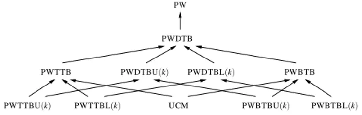
PW PWDTBU(k) PWDTBL(k) PWDTB UCM PWBTB PWBTBU(k) PWBTBL(k) PWTTB PWTTBU(k) PWTTBL(k)
Figure 1: A hierarchy of possible winner problems
PWTTB is closely related to, but different from, the decision problem EXTENSION-BRIBERYfor the zero-cost model. While in PWTTB we have to extend all votes to linear orders, in
EXTENSION-BRIBERYwe have the freedom to extend votes only
partially. Still, EXTENSION-BRIBERYreduces to PWTTB for each scoring rule in the optimistic scoring, zero-cost model.
Let k be a fixed positive constant. We consider the following re-striction of PWTTB to top-truncated ballots with upper-bounded
(lower-bounded) length k: For every top-truncated ballot B, the number of candidates ranked in B is at most k (at least k). The restriction of PWTTB to such ballots is denoted by PWTTBU(k) (PWTTBL(k)). Analogous definitions can be made for bottom-truncated and doubly-bottom-truncated ballots. Let the corresponding pos-sible winner problems with truncated ballots of either upper- or lower-bounded length be denoted by PWBTBU(k), PWBTBL(k), PWDTBU(k), and PWDTBL(k). Truncated ballots with upper-bounded length may be seen as being heavily truncated, whereas truncated ballots with lower-bounded length may be seen as be-ing only moderately truncated. Because UCM uses ballots that are either full or empty, neither PWTTBU(k) nor PWTTBL(k) is a more general problem than UCM. An analogous comment applies to PWBTBU(k), PWBTBL(k), PWDTBU(k), PWDTBL(k).
On the other hand, we immediately have from the definitions that UCM is a special case of both PWTTB and PWBTB, which in turn are special cases of PWDTB, and PWDTB is a special case of PW. This is stated in Proposition 4.1 and shown in Figure 1. In this figure, an arrow between two problems, A→ B, means that A (polynomial-time many-one) reduces to B.
PROPOSITION 4.1. Among the possible winner problems with
and without truncated ballots defined above, we have the reduc-tions shown in Figure 1.
Now, since the problems PWTTB, PWBTB, and PWDTB are sandwiched between PW and UCM (recall that UCM is a special case of PW), they immediately inherit any membership in P re-sult from PW and any NP-hardness rere-sult from UCM. Thus, from known results about the PW and UCM problems for common vot-ing rules [10, 25, 3, 33], we can classify these into three groups: (1) PW is in P for, e.g., plurality, veto, Condorcet, and plurality with runoff (in the co-winner case); (2) UCM is NP-hard for, e.g., Copeland, STV, maximin, ranked pairs, most scoring rules, plus all rules for which winner determination is NP-hard; (3) PW is NP-hard and UCM is in P for, e.g., Bucklin, voting trees, plurality with runoff (in the unique-winner case), and k-approval. Therefore, among the voting rules listed above, the complexity of PWTTB, PWBTB, and PWDTB is not yet known for Bucklin, voting trees, plurality with runoff (in the unique-winner case), and k-approval.
THEOREM 4.2. For k-approval, the problems PWDTB and, a
fortiori, PWTTB and PWBTB are in P.
PROOF. Let V= (v1, . . . , vn) be a given list of doubly-truncated
and bottom(vi) for each voter viin V . Let p∈ C be the distinguished
candidate. To decide whether p is a winner, we transform the given instance into the following network flow problem:
1. For each i, 1≤ i ≤ n, if top(vi) < k, and the position of p
is not revealed in vi (i.e., p is among the unranked
candi-dates in vi), then add p at position top(vi) + 1 in vi. Let
V′= (v′1, . . . , v′n) be the corresponding modified profile with
adjusted values top(v′i), 1 ≤ i ≤ n.
2. For each i, 1≤ i ≤ n: (a) if top(v′i) ≥ k, then let Zibe the set
containing the first k candidates of v′i; (b) if top(v′
i) < k and
bottom(v′i) ≤ m − k, then let Zibe the set containing the first
top(v′i) candidates of v′i; (c) if top(v′i) < k and bottom(v′i) >
m− k, then let Zibe the set cotaining the first top(v′i)
candi-dates plus the first bottom(v′i) − m + k candidates which are ranked at the bottom of v′i.
3. For each c∈ C, let S(c) = k{i | c ∈ Zi}k.
4. The flow network contains n+ m + 1 nodes: (a) one node c for each candidate c∈ C \ {p}, (b) one node v′ifor each voter
v′i∈ V′, (c) a source s, and (d) a sink t.
5. The flow network contains the following edges: (a) there is an edge from s to every c∈ C \{p} with capacity S(p)−S(c); (b) there is an edge from c∈ C \ {p} to v′i∈ V′with capacity 1 if and only if the position of c is not revealed in v′i; (c) there is an edge from every v′i∈ V′to t with capacity
0 if top(v′ i) ≥ k; k− top(v′
i) if top(v′i) < k and bottom(v′i) ≤ m − k;
m− top(v′i)
− bottom(v′i) if top(v′i) < k and bottom(v′i) > m − k. We claim that p is a possible winner in the k-approval election (C,V ) if and only if there is a flow of value ∑n
i=1aiin the network
constructed above, where (1) ai= 0 if top(v′i) ≥ k, (2) ai= k −
top(v′
i) if top(v′i) < k and bottom(v′i) ≤ m − k, and (3) ai= m −
top(v′i) − bottom(v′i) if top(v′i) < k and bottom(v′i) > m − k. Assume that p is a possible k-approval winner for(C,V ). That means that there is an extension of the list of truncated ballots V into a list W of complete ones such that p is a k-approval winner of election(C,W ). Without loss of generality, we can assume that
pis placed at the first possible position in each vote viwhere its
position is unrevealed. Let(C,V′) be the profile thus modified. The points every candidate gets in the profile(C,V′) correspond to the values S(c) of the above construction. We now show that there is a flow of value ∑ni=1aiin the network. First note that ∑ni=1aiis
the sum of the unranked candidates among the first k positions in all votes. Since no candidate gets more points than p in(C,W ), there is a flow of value at most S(p) − S(c) from s to every node
cfor each candidate c∈ C \ {p}. If in the list of complete ballots candidate c takes a position in a vote vithat was unrevealed in V′,
there is a flow of value one from c to vi. Further, from each node vi,
1≤ i ≤ n, there is a flow to the sink t whose value corresponds to the unrevealed candidates among the first k positions. Hence there is a flow of the desired value in this network.
Now assume that there is a flow of value ∑ni=1aiin the network.
For the given election(C,V ), we again first place candidate p at the first possible position in the votes where its position was unrevealed before, and we refer to the modified profile by V′. If there is a flow of value one from node c to vi, candidate c is placed among the first
kpositions in vote vi. The sum of all aiensures that all first k
posi-tions are taken in all votes, and the capacity of S(p) − S(c) from the source s to the nodes corresponding to the candidates c∈ C \ {p}
ensures that no candidate can get more points than p. Hence, com-pleting the profile V′as described results in a k-approval election in which p is a winner.
5.
RELATED WORK
Although most of the literature in voting theory assumes that votes are full linear orders, truncated ballots have been considered in a few papers. Brams and Sanver [7] consider ballots that consist of ranked lists of approved candidates (i.e., of possibly truncated ballots), and they propose two specific ways of aggregating them, namely preference approval voting and fallback voting. Aggregat-ing truncated ballots also appears in a stream of work in database theory, where aggregating ordered lists of results to queries (pro-vided by web search engines, for example) corresponds to aggre-gating several ordered lists in which, typically, every element ap-pears only in some lists, not in all (see, e.g., [12, 17, 1]). Assuming that the elements that are not ranked in a list are considered less relevant than the elements that appear in it, it is clear that the prob-lem consists in aggregating a set of top-truncated rankings into a complete ranking. The aggregation rules used in this community are median rankings, which minimize some distance to the ballots, such as, typically, the Kemeny rule. One reason why these median ranking rules are used by this community is that their definition ex-tends in a straightforward way to truncated rankings. Here we focus on other rules, and we also show that any other possible rule can be extended in a systematic way to truncated ballots, by considering all possible extensions of the truncated ballots. Rank aggregation with partial information is also important in peer-reviewing [30], and it received considerable attention from the machine learning community. For example, doubly-truncated votes are a special case of a similar notion studied by Lebanon and Mao [26]. Finally, En-driss et al. [16] provide a general approach to voting with many kinds of ballots, including truncated ballots.
Section 3 deals with the issue of campaign management for the case of truncated votes. Campaign management as a computa-tional problem appeared, e.g., in [13, 31]. In particular, the latter work considered the problem SUPPORT-BRIBERYwhere the cam-paign manager can extend votes. However, there the voters already have fixed preference orders, whereas in EXTENSION-BRIBERY
the manager has the freedom to ask the voters to additionally rank any subset of candidates in any order. In this sense EXTENSION -BRIBERYis similar to the BRIBERYproblem [18], except that in BRIBERYif we buy a given vote, we can rewrite it completely.
Section 4 relates to computing possible winners. This notion has been introduced by Konczak and Lang [25] and has been studied from a computational point of view (see, e.g., [33, 3, 29]). The relation to preference elicitation is further explored by Walsh [32]. Parameterized complexity results for the possible winner problem are given by Betzler et al. [4]. Kalech et al. [24] design voting pro-tocols in which agents submit their preferences incrementally, in rounds, and study experimentally the probability that there exists a necessary winner given the amount of information known. Lu and Boutilier [27] use minimax regret to output a robust winner given incomplete preferences, which is a way of coping with the possi-bly high number of possible winners. Xia and Conitzer [34] use the maximum likelihood approach to define voting rules form in-complete votes. Finally, a restricted variant of the possible winner problem, where the incompleteness of the profile comes from the fact that some alternatives were not known initially, is the
possi-ble winner propossi-blem with respect to the addition of new alternatives
(PWNA) [9, 35, 2]. In PWNA, each voter has a full linear order over the set C of “known” candidates, but there is also a set A of ad-ditional candidates. The question is whether it is possible to extend
the linear orders of the voters to rank all the candidates in C∪ A, so that some given candidate is a winner. At first sight it may look as if PWNA were a subproblem of PWTTB, PWBTB, and PWDTB. However, in the PWNA problem the remaining alternatives can be ranked anywhere, whereas in the case of truncated ballots they have to come between the ranked top and ranked bottom candidates.
6.
CONCLUSIONS AND FUTURE WORK
We have studied various aspects of elections when the input votes are truncated rankings consisting of a ranked list of top can-didates and/or a ranked list of bottom cancan-didates. We proposed ways of extending some voting rules to truncated ballots, and have addressed the complexity of the problem of persuading voters to extend their votes so as to ensure that a given candidate wins. Con-sidering truncated ballots as incompletely specified rankings, we showed that determining possible winners makes sense in this set-ting. While the complexity of the possible winner problem for trun-cated ballots follows from known results for many voting rules, we provided an efficient algorithm in one of the few other cases.
The generalization of voting rules to truncated ballots, and the study of such generalizations, deserves more attention. One goal is to extend common social-choice-theoretic properties to truncated ballots and to see if the properties fulfilled by a voting rule are still fulfilled in this generalization. Introducing new properties ap-plicable only to (properly) truncated ballots may also make sense. Considering truncated ballots as incomplete ballots, how likely is it that the result is determined (i.e., that there exists a necessary win-ner) when all voters have specified ballots of a given size? (Kalech et al. [24] address a similar question in a different setting.) It is ob-vious how to prove that for the Bucklin rule: If top lists are of size ⌈m/2⌉ then there exists a necessary winner. It may also be
interest-ing to build elicitation protocols so as to ask voters to expand their truncated ballots in a minimal way, in terms of the number of bits exchanged, so that the outcome of the vote is determined. Finally, we still have to address the complexity of PWDTB for plurality with runoff (in the unique-winner case), voting trees, and Bucklin.
Acknowledgements. We thank the referees for their many useful
comments. This work was supported in part by DFG grant RO-1202/15-1, SFF grant “Cooperative Normsetting” of HHU Düssel-dorf, a DAAD/MAEE/MESR grant for a project in the PROCOPE programme, AGH Univ. of Technology grant 11.11.120.865, the Foundation for Polish Science’s Homing/Powroty program, and the ANR project ComSoc (ANR-09-BLAN-0305).
7.
REFERENCES
[1] N. Ailon. Aggregation of partial rankings, p-ratings and top-m lists.
Algorithmica, 57(2):284–300, 2010.
[2] D. Baumeister, M. Roos, and J. Rothe. Computational complexity of two variants of the possible winner problem. In Proc. AAMAS-11, pages 853–860, May 2011.
[3] N. Betzler and B. Dorn. Towards a dichotomy of finding possible winners in elections based on scoring rules. Journal of Computer and
System Sciences, 76(8):812–836, 2010.
[4] N. Betzler, S. Hemmann, and R. Niedermeier. A multivariate complexity analysis of determining possible winners given incomplete votes. In Proc. IJCAI-09, pages 53–58, July 2009. [5] N. Betzler, R. Niedermeier, and G. Woeginger. Unweighted
coalitional manipulation under the Borda rule is NP-hard. In Proc.
IJCAI-11, pages 55–60, July 2011.
[6] M. Bläser. Computing small partial coverings. Information
Processing Letters, 85(6):327–331, 2003.
[7] S. Brams and R. Sanver. Voting systems that combine approval and preference. In S. Brams, W. Gehrlein, and F. Roberts, editors, The
Mathematics of Preference, Choice, and Order: Essays in Honor of Peter C. Fishburn, pages 215–237. Springer, 2009.
[8] M. Cesati. The Turing way to parameterized complexity. Journal of
Computer and System Sciences, 67(4):654–685, 2003.
[9] Y. Chevaleyre, J. Lang, N. Maudet, and J. Monnot. Possible winners when new candidates are added: The case of scoring rules. In Proc.
AAAI-10, pages 762–767, July 2010.
[10] V. Conitzer, T. Sandholm, and J. Lang. When are elections with few candidates hard to manipulate? J.ACM, 54(3):Article 14, 2007. [11] J. Davies, G. Katsirelos, N. Narodytska, and T. Walsh. Complexity of
and algorithms for Borda manipulation. In Proc. AAAI-11, pages 657–662, Aug. 2011.
[12] C. Dwork, R. Kumar, M. Naor, and D. Sivakumar. Rank aggregation methods for the web. In Proc. WWW-01, pages 613–622, Mar. 2001. [13] E. Elkind and P. Faliszewski. Approximation algorithms for
campaign management. In Proc. WINE-10, pages 473–482, 2010. [14] E. Elkind, P. Faliszewski, and A. Slinko. Cloning in elections:
Finding the possible winners. JAIR, 42:529–573, 2011. [15] P. Emerson. The original Borda count and partial voting. Social
Choice and Welfare. To appear.
[16] U. Endriss, M. Pini, F. Rossi, and K. Venable. Preference aggregation over restricted ballot languages: Sincerity and strategy-proofness. In
Proc. IJCAI-09, pages 122–127, July 2009.
[17] R. Fagin, R. Kumar, and D. Sivakumar. Comparing top k lists. SIAM
Journal on Discrete Mathematics, 17(1):134–160, 2003.
[18] P. Faliszewski, E. Hemaspaandra, and L. Hemaspaandra. How hard is bribery in elections? JAIR, 35:485–532, 2009.
[19] P. Faliszewski, E. Hemaspaandra, and L. Hemaspaandra. Using complexity to protect elections. C.ACM, 53(11):74–82, 2010. [20] P. Faliszewski, E. Hemaspaandra, and H. Schnoor. Manipulation of
Copeland elections. In Proc. AAMAS-10, pages 367–374, 2010. [21] P. Faliszewski and A. Procaccia. AI’s war on manipulation: Are we
winning? AI Magazine, 31(4):52–64, 2010.
[22] U. Feige. A threshold of ln n for approximating set cover. J.ACM, 45(4):634–652, 1998.
[23] E. Hemaspaandra, L. Hemaspaandra, and J. Rothe. Anyone but him: The complexity of precluding an alternative. Artificial Intelligence, 171(5–6):255–285, 2007.
[24] M. Kalech, S. Kraus, G. Kaminka, and C. Goldman. Practical voting rules with partial information. JAAMAS, 22(1):151–182, 2011. [25] K. Konczak and J. Lang. Voting procedures with incomplete
preferences. In Proc. Multidisciplinary IJCAI-05 Workshop on
Advances in Preference Handling, pages 124–129, July/Aug. 2005. [26] G. Lebanon and Y. Mao. Non-parametric modeling of partially
ranked data. J. Machine Learning Research, 9:2401–2429, 2008. [27] T. Lu and C. Boutilier. Robust approximation and incremental
elicitation in voting protocols. In Proc. IJCAI-11, pages 287–293, July 2011.
[28] R. Niedermeier. Invitation to Fixed-Parameter Algorithms. Oxford University Press, 2006.
[29] M. Pini, F. Rossi, K. Venable, and T. Walsh. Possible and necessary winners in voting trees: Majority graphs vs. profiles. In Proc.
AAMAS-11, pages 1–9, May 2011.
[30] M. Roos, J. Rothe, and B. Scheuermann. How to calibrate the scores of biased reviewers by quadratic programming. In Proc. AAAI-11, pages 255–260, Aug. 2011.
[31] I. Schlotter, P. Faliszewski, and E. Elkind. Campaign management under approval-driven voting rules. In Proc. AAAI-11, pages 726–731, Aug. 2011.
[32] T. Walsh. Uncertainty in preference elicitation and aggregation. In
Proc. AAAI-07, pages 3–8, July 2007.
[33] L. Xia and V. Conitzer. Determining possible and necessary winners given partial orders. JAIR, 41:25–67, 2011.
[34] L. Xia and V. Conitzer. A maximum likelihood approach towards aggregating partial orders. In Proc. IJCAI-11, pages 446–451, July 2011.
[35] L. Xia, J. Lang, and J. Monnot. Possible winners when new alternatives join: New results coming up! In Proc. AAMAS-11, pages 829–836, May 2011.