GENERATION OF HDR IMAGES IN NON-STATIC CONDITIONS
BASED ON GRADIENT FUSION
Keywords: High Dynamic Range Images, Gradient Fusion, Registration, Optical Flow.
Abstract: We present a new method for the generation of HDR images in non-static conditions, i.e. hand held camera and/or dynamic scenes, based on gradient fusion. Given a reference image selected from a set of LDR pictures of the same scene taken with multiple time exposure, our method improves the detail rendition of its radiance map by adding information suitably selected and interpolated from the companion images. The proposed technique is free from ghosting and bleeding, two typical artifacts of HDR images built through image fusion in non-static conditions. The advantages provided by the gradient fusion approach will be supported by the comparison between our results and those of the state of the art.
1
INTRODUCTION
Radiance in natural scenes can span several orders of magnitude, yet commercial cameras can capture only two orders of magnitude and reproduce Low Dy-namic Range (LDR) photographs, often affected by saturated areas and loss of contrast and detail. Dur-ing the last fifteen years, many techniques have been studied and proposed in order to expand the dynamic range of digital photographs to create the so-called High Dynamic Range (HDR) images, i.e. matrices whose entries are proportional to the actual radiance of the scene. For a thorough overview of the HDR imaging we refer the interested reader to the excellent book (Reinhard et al., 2005).
Two main problems remain to be solved in HDR imaging. First, while the technique proposed by De-bevec and Malick (DeDe-bevec and Malik, 1997) can be considered as the ‘de facto standard’ for the creation of HDR images in static conditions, i.e. with perfectly still camera and without moving objects in the scene, no standard is available when these condition fail. Second, HDR images cannot be entirely displayed or printed on the majority of commercial screens or printers, hence a so-called ‘Tone-Mapping’ transfor-mation is needed to properly reduce their range with-out losing details and respecting as much as possible the original color sensation.
In this paper we deal only with the first problem, i.e. we study HDR image generation in non-static conditions, which are, by far, the most common. As we will explain in more detail later on, standard HDR image creation algorithms assume perfect alignment for the input images and no motion, the price to pay when this assumption fails is the generation of
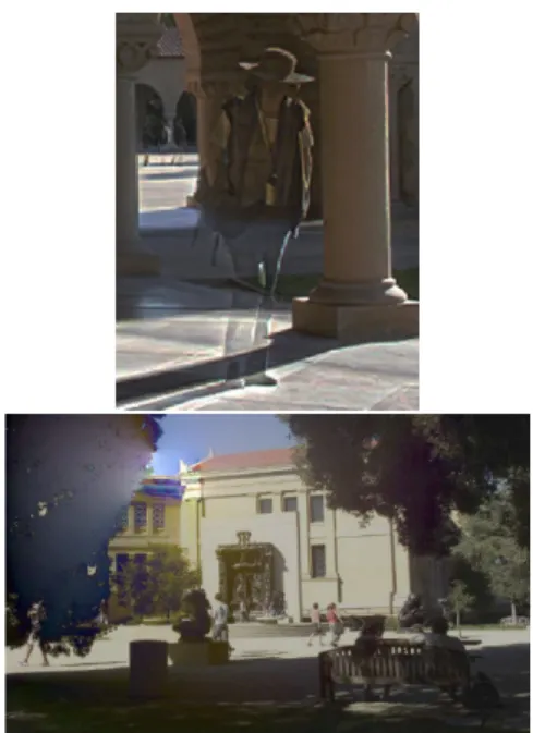
arti-facts, in particular those called ‘ghosts’, i.e. objects with a translucent appearance induced by an incoher-ent image fusion, and ‘bleeding’, i.e. the diffusion of an artificial color over a flat image region, see Fig-ure 1. To avoid this and other problems that we will discuss in more detail later, instead of synthesizing a new HDR image from the original sequence of LDR images, we will select just one of them to be the
ref-erence and then we will improve the associated
radi-ance map by adding as many details as possible with-out introducing artifact. In doing this, a fundamental role will be played by gradient fusion, which has sev-eral advantages with respect to intensity fusion in this case. As we will show in Section 5, the results of the proposed technique compare well to the state of the art.
2
STATE OF THE ART IN HDR
IMAGE CREATION
For the sake of readability, it is worthwhile to be-gin this section by introducing some concepts and no-tation that will be used throughout the paper. We define the radiance E(x) to be the electromagnetic power per unit of area and solid angle that reaches the pixel x of a camera sensor with spatial supportΩ ⊂ R2. The camera response function f is the non-linear
mapping f : [0, +∞) → {0,...,255} that transforms the radiance E(x) acquired in the time∆t into I(x), the
intensity value of the pixel x, i.e. f (E(x)∆t) = I(x). f
is assumed to be semi-monotonically increasing, i.e. its derivative is supposed to be non-negative, since the digital values stored by the camera remain
con-Figure 1: From top to bottom: an example of ghost and bleeding artifacts, respectively.
stant or increase as the radiance increases. In par-ticular, the graph of f remains constant to 0 (black) for all the radiance values that do not overcome the sensibility threshold of the camera sensor and to 255 (white) for all those radiance values that exceed its saturation limit. For values that lie inside these two extremes, f is invertible and so we can use its inverse
f−1:{0,...,255} → [0,+∞) to pass from image in-tensity values I(x) to the corresponding radiance val-ues E(x): f−1(I(x)) = E(x)∆t. The camera response function can be built in controlled conditions by tak-ing photos of a uniformly illuminated Macbeth chart with patches of known reflectance.
However, in many practical cases, the camera re-sponse function is not known, thus various techniques for recovering f or its inverse without a Macbeth chart have been developed. These methods are called
chart-less and are all based on the same principle: since
the camera sensor is limited by its sensibility thresh-old and saturation limit, in order to detect the whole scene radiance one has to take N≥ 2 shots with dif-ferent time exposures ∆tj, j = 1, . . . , N. The next
step consists in using the redundant information about the scene provided by the set of N digital images
Ij to recover the inverse camera function f−1. This
is the only step that distinguishes the various algo-rithms proposed in the HDR imaging literature that we will briefly recall later. Let us for the moment sup-pose that we have indeed computed f−1, then we can construct the j-th partial radiance Ej(x) as follows:
Ej(x)≡ f−1(Ij(x))
/
∆tj, j = 1, . . . , N. Notice that we
use the adjective ‘partial’ when referring to the radi-ances Ejbecause they are built by applying f−1to Ij,
thus Ejcannot be considered a faithful representation
of the entire radiance range, but only of the part cor-responding to clearly visible details in the j-th image. Finally, in order to compute the set of final radiance values{E(x), x ∈ Ω} that will constitute the HDR im-age of the scene, one performs a weighted averim-age of the partial radiances:
E(x) =∑ N j=1w(Ij(x))Ej(x) ∑N j=1w(Ij(x)) , (1)
where the weights w take their maximum in 127, the center of the LDR dynamic range, and decrease as the intensity values approach 0 or 255, when the infor-mation provided by Ij is imprecise. If one deals with
color images, then this procedure must be repeated
three times in order to recover three radiance func-tions relative to the red, green and blue spectral picks of the scene radiance.
As we have said, the algorithms for HDR im-age generation in static conditions are practically dis-tinguished only for how they recover inverse cam-era response function f−1. Mann and Picard (Mann and Picard, 1995; Mann, 2000) were the first to ad-dress this problem, they postulated a gamma-like an-alytical expression for f−1 and solved a curve fit-ting problem to determine the most suitable param-eters. Mitsunaga and Nayar (Mitsunaga and Nayar, 1999) improved Mann and Picard’s work by assum-ing f−1 to be a polynomial and determining its co-efficients through a regression model. Debevec and Malik (Debevec and Malik, 1997) worked with log-arithmic data and did not impose any restrictive an-alytic form to f−1, yet they required it to be smooth by adding a penalization term proportional to the sec-ond derivative of f−1 to the following optimization problem: Minklog f−1(Ij(x))− logE(x) − log∆tjk2.
Their method is fast and gives reliable results, for this reason it has become the de facto standard in the field of HDR imaging with static conditions.
Let us now consider non static conditions, i.e. im-ages taken with hand held camera and/or of dynamic scenes. In this case, a motion detection step must be added to register the set of input LDR images and a more careful fusion process must be considered to avoid artifacts.
Let us begin with registration: Ward (Ward, 2003) proposes to use multi-scale techniques to register a set of Median Threshold Maps (MTB), which are a bi-narization of the images with respect to their median value. Although this approach is independent of the exposure time, it depends on noise and histogram den-sity around the median value. Grosch (Grosch, 2006)
bases a local registration method on Ward’s MTBs and Jacobs et al. (Jacobs et al., 2008) proposed an improvement of Ward’s work by estimating motion with an entropy based descriptor. These methods give good results for the case of small movements gener-ated by a hand held camera, but they tend to produce artifacts when dealing with large object motion, as e.g. people walking through the scene. Tomaszewska and Mantiuk (Tomaszewska and Mantiuk, 2007) and Heo et al. (Heo et al., 2011) propose to compute a global homography using RANSAC with SIFT de-scriptors which are based on gradients. Finally, Kang et al. (Kang et al., 2003) propose to use the camera function to boost the original images in order to facil-itate the registration process.
Let us consider now the methods that focus mainly on a suitable improvement of the fusion step. As we have said before, if we assume a perfect corre-spondence among pixels in non-static conditions and perform a weighted average of radiances, then ghosts artifacts appear in areas where motion has occurred. Many methods in the state of the art, e.g. (Khan et al., 2006), (Heo et al., 2011), (Granados et al., 2010), (Grosch, 2006) and (Jacobs et al., 2008), focus on avoiding ghost formation by modifying eq. (1) in or-der to reduce the influence of pixels corresponding to moving objects in the process of intensity fusion to generate the HDR image. These methods may be ro-bust to pixel saturation and small misalignments, but the areas that appear only in one image will be copied while the other image areas will be averaged from dif-ferent images, thus new boundaries could be created in the process. In order to deal with these artifacts, Gallo et al. (Gallo et al., 2009) propose to create a vector field by copying patches of gradients from the best exposed areas that match a reference image. Then they blend the borders of neighboring patches and integrate the vector field. The resulting images are ghost free but artifacts appear on the patch borders and flat regions. Finally, let us report that gradient-based methods can deal with the radiance differences among the image sequence but are sensitive to mis-alignments and can produce color bleeding as Eden et al. (Eden et al., 2006) have pointed out.
3
THE PROPOSED ALGORITHM
The method that we propose has several steps in cascade, before describing in detail all the steps it is worthwhile to give a brief summary of the whole al-gorithm. Firstly, as done in the static scenario, we ap-ply the inverse camera function to every LDR image of the bracketing of pictures taken with different time
exposures, obtaining the partial radiance map for each one of them. These radiance maps are radiometrically aligned using the camera function with the exposure time of the reference image. These modified images are used to compute a dense correspondence field, us-ing the optical flow algorithm of Chambolle and Pock (Chambolle and Pock, 2011), for every image with respect to the reference one. These correspondences are subsequently filtered using a refinement step: for every pair of images, we compensate the motion be-tween them and compute the absolute value image difference. The histogram of this image difference is modeled as a mixture of Gaussians, which allows us to distinguish between correct and erroneous corre-spondences. Finally, we use the corrected correspon-dences to obtain a gradient field that we integrate by solving a Poisson equation. To avoid color bleeding and other color artifacts we set a randomly selected group of points as Dirichlet boundary conditions. The intensity values of these points are computed through the Debevec-Malik intensity fusion of the aligned pix-els.
The first step of the algorithm has already been de-scribed in the previous section, we present and discuss the following steps in separated subsections.
3.1
RADIANCE REGISTRATION
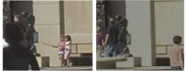
As previously declared, the goal of our method is to increase the detail rendition of the reference radiance map in the areas where the original LDR reference image was over/under exposed. The aim is to obtain these missing details from other images of the brack-eting without creating artifacts produced by merging motion pixels. Thus, we need to distinguish motion pixels that we do not want to fuse from details that appear in other images (but not in the reference one) that we actually want to fuse. To explain the problem let us consider the two HDR radiance maps shown in Figure 2.
Figure 2: Radiance maps of two pictures shown with the software HDRshop (available online at http://www.hdrshop.com/) useful to exemplify the ra-diance registration process (images courtesy of O.Gallo).
From the two images in Figure 2 we take the right one as reference. In this case we would like to
intro-duce the detail of the texture on the wall present in the left image, avoiding the girls that cover it, given that we want to maintain the scene of the reference image. A registration algorithm based on intensity or geometry comparison cannot distinguish between wall details and people passing by, thus we need to modify the radiance maps before operating the regis-tration, in such a way that the pixels corresponding to wall details are matched for fusion but not those cor-responding to the girls. More generally, we need a
pre-registration step that modifies the radiance maps
so that the registration process will match the most precise details, i.e. those coming from dark areas of overexposed images and from bright areas of under-exposed images.
Our tests have shown that the more efficient ra-diometric modification for this scope is given by the application of the camera response function with the (fixed) time exposure of the reference image, to each radiance map, as also observed by (Kang et al., 2003). Thus instead of Ij we work with the modified
im-ages f (∆trefEj(x)). Notice that the reference image
remains unchanged while for the others the transfor-mation amounts to a normalization of the exposure time. Notice that, since the range of f is{0,...,255}, after this process the radiance maps become a new set of LDR images. The advantage of this transformation is that the intensity levels become closer and that the image areas corresponding to the over/under-exposed values of the reference image also appear saturated in the other radiometrically aligned images.
After this pre-registration step, we can apply any optical flow method over the new set of LDR images. We used the method of Chambolle and Pock (Cham-bolle and Pock, 2011) which provides dense corre-spondences between pixels. Although the matchings are accurate, the method can produce errors on the boundaries of moving objects and the areas where ob-jects disappear due to motion. Thus a refinement step is needed to check whether the correspondences are correct or not.
3.1.1 REFINEMENT STEP
Let us assume that we have two radiometrically aligned images Iref, Ij, j = 1, . . . , N, without motion.
The pixel-wise distance between them defines the dif-ference imagekIref(x)− Ij(x)k that depends on their
noise. If we model this noise as additive and Gaus-sian, then the difference image histogram will be highly populated close to zero. As the motion (or mis-matches) among the images increases, more modes appear in this histogram. We therefore propose mod-eling this difference histogram as a set of Gaussians using a Gaussian Mixture Model (GMM) where the
most probable Gaussian is associated to the prop-erly matched pixels and the other Gaussians represent matchings that are not correct. Let the most proba-ble Gaussian be characterized by a median µ and a standard deviationσ. We define as a mismatch those correspondences with a distance from µ given byασ, whereα is a parameter of the algorithm. After the re-finement step, a pixel of the reference radiance map can have a set of correspondences in pixels of the other images of the sequence or no correspondence at all if the pixel belongs to an object that appears only in the reference image.
4
GRADIENT FUSION
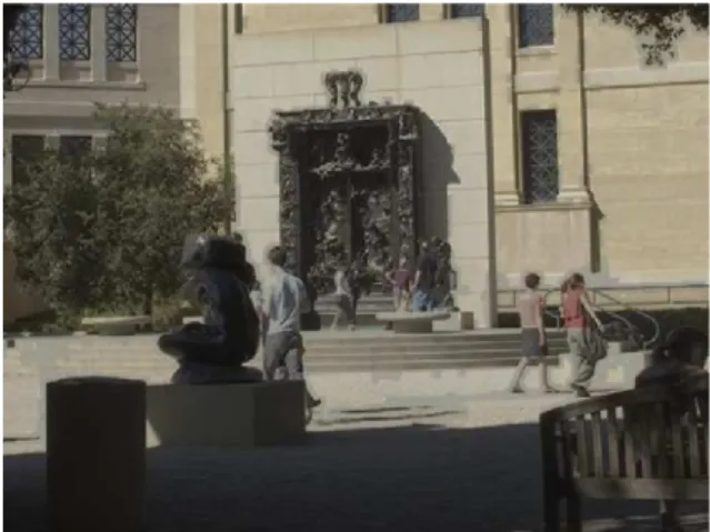
After the steps previously discussed we know which pixels can be fused without generating artifacts in the final HDR image. Here we examine the pro-cess that will add details to the reference radiance map from the others in the set. Let us begin by observing that in general we do not have correspondences be-tween all pixels of the reference image and pixels in all the other images of the bracketing, thus an inten-sity fusion can create artificial edges, as can be seen in Figure 3.
Figure 3: Detail of a result obtained by building radiance maps with an intensity fusion process, it can be seen that artificial edges appear (in particular around the moving peo-ple). Image (courtesy of O. Gallo) shown with HDRShop at a fixed time exposure.
Note that the people are moving along the se-quence, thus, their intensity values are being copied from the reference image to the final image while the other areas are computed by a weighted average among the corresponding pixels. This difference gen-erates new edges around the subjects in motion. In order to avoid this problem, we propose using gradi-ent fusion techniques in the Log-scale. Let us set for
this scope ˜Ij= log10(Ij), j = 1, . . . , N.
Poisson Editing (P´erez et al., 2003) allows
mod-ifying the features of an image without creating new edges or artifacts in the LDR domain. The idea is to copy a target gradient field in a regionΩ0 of the image domain which is then integrated by solving a Poisson equation. Thus, the problem is to properly choose the target gradient field. To do that, recall that our aim is to improve the detail rendition of the fi-nal HDR image, so we must give more importance to gradients with largest norm. As discussed in (Piella, 2009), if we consider the weighted second moment matrix Gs(x): Gs(x) = ∑ N j=1 ( sj(x)∂x∂˜I 1 )2 ∑N j=1s 2 j(x)∂x∂˜I1∂x∂˜I2 ∑N j=1s2j(x)∂x∂˜I2 ∂˜I ∂x1 ∑ N j=1 ( sj(x)∂x∂˜I2 )2 (2) where the partial derivatives are com-puted at the point x = (x1, x2) and sj(x) =
k∇˜Ij(x)k
/√ ∑N
i=1k∇˜Ii(x)k2, then the
predom-inant gradient direction is given by the largest eigenvector of Gs(x) and the corresponding
eigen-value gives its norm. In this process the sign of the gradient is lost. In our experiments, we have seen that the best results are achieved when we restore the sign to be that of the gradient with maximum modulus.
We can now define the target vector field for Pois-son editing as follows: given a pixel x in the reference image, from all gradients of the bracketing of images at x, we select the gradient with largest modulus. Let us denote it by M(x). Then the target vector V in x is defined as:
V (x) =√λε(x)θ, (3) whereλ is the largest eigenvalue of Gs(x),θ its
asso-ciated eigenvector, and ε(x) =
{
−1 if hθ,M(x)i ≤ 0;
1 otherwise.
We stress that V (x) is not necessarily a conservative vector field and, as remarked by Tao et al. (Tao et al., 2010) this can lead to bleeding effects along strong edges. In order to stop the bleeding effect, we have introduced Dirichlet boundary conditions at a set of randomly chosen points ofΩ taken from the set of points for which there exist reliable correspondences. For them we have set the intensity as the radiance ob-tained with the Debevec-Malik intensity fusion.
5
RESULTS AND COMPARISONS
Now that the method has been described we can proceed to give some implementation detail. The
op-tical flow method of Chambolle and Pock was ap-plied to the luminance values of the radiometrically aligned images. For the refinement step we modeled the histogram of image differences as a GMM (Gaus-sian Mixture Model) with two components. A final step in the refinement process is introduced to avoid taking into account pixels on the boundaries: inter-preting the mismatches as motion masks, we apply to these masks a dilation filter with a 6× 6 structuring element (Gonzales and Woods, 2002). In the fusion process we randomly select the 10% of the total image area as possible Dirichlet points keeping only those with matches. Finally, we solve the Poisson equation using the Conjugate Gradient method for each color channel independently.
Let us now discuss the results of our proposal. Since HDR images cannot be represented on a LDR display, to show the results obtained from our algo-rithm we will show snapshots of the image provided by the free HDRShop software, available online at www.hdrshop.com, at a given exposure time. The comparison with the state of the art will be done fol-lowing the procedure used in other papers, that is, by comparing the tone mapped versions of the HDR im-ages.
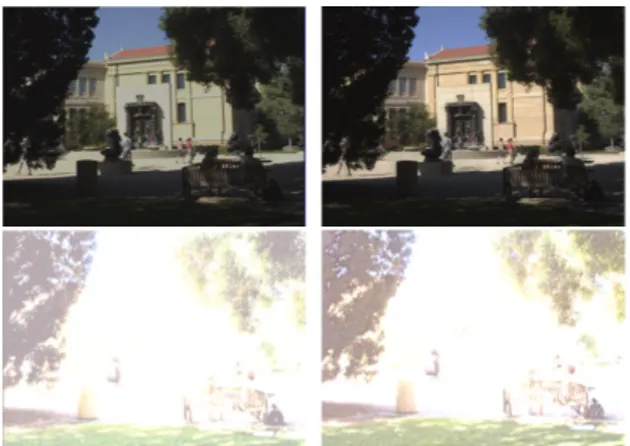
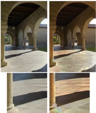
First of all we would like to start by showing the improvement obtained using our method. In Figure 4 we can see two original partial radiance maps com-pared to our results. The enhancement is specially obvious on the building wall (first row), where our method recovers texture and color, and also in the trees, which show much more details (second row).
Figure 4: Left column: original reference radiance map at two different time exposures set in the HDRshop soft-ware. Right column: corresponding enhanced image with the method proposed in the paper. The parameterα was set to 1.
The parameterα controls the flexibility in the se-lection of matches in the registration process. Our experiments have shown that a value ofα that gives
overall good performances is 0.5, for which we have found no artifacts in the final images. As we approach 1 we generate more details, but we might also create artifacts, as can be seen in Figure 5.
Figure 5: From left to right: results of our algorithm ob-tained by settingα = 0.5 (no artifacts) and α = 1 (artifacts appear), respectively.
The selection of the reference image can also in-fluence the appearance of ghosts or artifacts. We have in fact observed that when a moving pixel with a color similar to the background is located in an area satu-rated by the camera function, then the refinement step may fail to distinguish background from foreground and color artifacts may appear. We can see an exam-ple in Figure 6: in the first row we present two images of the bracketing that were used as two different ref-erence images. The corresponding results are shown in the second row. In both cases the parameter value isα = 1. Note that the result shown on the left hand side has an artifact on the puppet’s leg. The reason is that the reference image is saturated in that area, so the refinement step cannot distinguish between the puppet’s leg and the ball.
Figure 6: First row: two different original images taken as reference. Second row: output of our algorithm. It can be noticed an artifact in the left hand image due to the failure of the refinement step explained in the text.
Finally, we show the comparison between our
re-sults and those of Gallo et al. (Gallo et al., 2009) who also use a gradient fusion technique. Since they present their results using tone mapped versions of their images, we also used a tone mapped version of ours. In Figure 7 we can see that our method avoids the generation of geometry artifacts as well as bleed-ing.
Figure 7: First row, from left to right: tone mapped results of our HDR generation model and that of Gallo et al., re-spectively. Second row: detail magnification of the pictures above. The color difference is due to the different tone map-ping operators used. We stress that the artifact visible in the image of Gallo et al’s is not produced by the tone mapping operator, but by their HDR formation model.
6
CONCLUSIONS
We have proposed a method for HDR image cre-ation in the non-static scenario where photographs have been taken with a moving hand-held camera and/or the scene to be captured is dynamic. Our method is based on gradient fusion techniques that compares well to the state of the art. We have com-puted reliable correspondences by analyzing the dif-ferences of registered images using a GMM model. We have pointed out the importance of using gradient-based method instead of intensity-gradient-based methods. Fi-nally, we proposed a technique in which a suitable selection of Dirichlet conditions permits to avoid or strongly reduce the bleeding artifacts that may appear after the integration of vector fields.
ACKNOWLEDGEMENTS
The authors would like to thank Dr. Orazio Gallo for kindly providing his images.
REFERENCES
Chambolle, A. and Pock, T. (2011). A first-order primal-dual algorithm for convex problems with applications to imaging. Journal of Mathematical Imaging and
Vi-sion, 40(1):120–145.
Debevec, P. and Malik, J. (1997). Recovering high dynamic range radiance maps from photographs. In Proc. of
the 24th annual conf. on Computer graphics, pages
369–378.
Eden, A., Uyttendaele, M., and Szeliski, R. (2006). Seam-less image stitching of scenes with large motions and exposure differences. In Computer Vision and
Pat-tern Recognition, 2006 IEEE Computer Society Con-ference on, volume 2, pages 2498–2505.
Gallo, O., Gelfand, N., Chen, W., Tico, M., and Pulli, K. (2009). Artifact-free high dynamic range imag-ing. IEEE International Conference on Computa-tional Photography (ICCP).
Gonzales, R. and Woods, R. (2002). Digital image
process-ing. Prentice Hall.
Granados, M., Ajdin, B., Wand, M., Theobalt, C., Seidel, H.-P., and Lensch, H. (2010). Optimal hdr reconstruc-tion with linear digital cameras. In 2010 IEEE
Con-ference on Computer Vision and Pattern Recognition (CVPR), pages 215–222.
Grosch, T. (2006). Fast and robust high dynamic range im-age generation with camera and object movement. In
Vision, Modeling and Visualization, RWTH Aachen,
pages 277–284.
Heo, Y., Lee, K., Lee, S., Moon, Y., and Cha, J. (2011). Ghost-free high dynamic range imaging. In Computer
Vision - ACCV 2010, volume 6495 of Lecture Notes in Computer Science, pages 486–500. Springer
Berlin-Heidelberg.
Jacobs, K., Loscos, C., and Ward, G. (2008). Automatic high-dynamic range image generation for dynamic scenes. IEEE Computer Graphics and Applications, 28:84–93.
Kang, S., Uyttendaele, M., Winder, S., and Szeliski, R. (2003). High dynamic range video. ACM Trans. Graph., 22:319–325.
Khan, E., Akyuz, A., and Reinhard, E. (2006). Ghost re-moval in high dynamic range images. In IEEE
In-ternational Conference on Image Processing, pages
2005–2008.
Mann, S. (2000). Comparametric equations with practi-cal applications in quantigraphic image processing.
Image Processing, IEEE Transactions on, 9(8):1389–
1406.
Mann, S. and Picard, R. W. (1995). On being undigital with digital cameras: Extending dynamic range by
com-bining differently exposed pictures. In Proceedings of
IS&T, pages 442–448.
Mitsunaga, T. and Nayar, S. (1999). Radiometric self cal-ibration. In Computer Vision and Pattern
Recogni-tion, 1999. IEEE Computer Society Conference on.,
volume 1, pages 374–380 Vol. 1.
P´erez, P., Gangnet, M., and Blake, A. (2003). Poisson im-age editing. In ACM SIGGRAPH 2003 Papers, pim-ages 313–318.
Piella, G. (2009). Image fusion for enhanced visualization: A variational approach. International Journal of
Com-puter Vision, 83:1–11.
Reinhard, E., Ward, G., Pattanaik, S., and Debevec, P. (2005). High Dynamic Range Imaging, Acquisition,
Display, And Image-Based Lighting. Morgan
Kauf-mann Ed.
Tao, M., Johnson, M., and Paris, S. (2010). Error-tolerant image compositing. In Proceedings of the 11th
Euro-pean conference on Computer vision: Part I, ECCV
2010, pages 31–44.
Tomaszewska, A. and Mantiuk, R. (2007). Image regis-tration for multi-exposure high dynamic range image acquisition. In Proc. Intl. Conf. Central Europe on
Computer Graphics, Visualization, and Computer Vi-sion (WSCG).
Ward, G. (2003). Fast, robust image registration for com-positing high dynamic range photographs from hand-held exposures. Journal of graphic tools, 8:17–30.