Rheological behavior and modeling of waxy crude oils in transient flows

(1)

HAL Id: tel-01235326

https://pastel.archives-ouvertes.fr/tel-01235326

Submitted on 30 Nov 2015

HAL is a multi-disciplinary open access archive for the deposit and dissemination of sci-entific research documents, whether they are pub-lished or not. The documents may come from teaching and research institutions in France or abroad, or from public or private research centers.

L’archive ouverte pluridisciplinaire HAL, est destinée au dépôt et à la diffusion de documents scientifiques de niveau recherche, publiés ou non, émanant des établissements d’enseignement et de recherche français ou étrangers, des laboratoires publics ou privés.

Rheological behavior and modeling of waxy crude oils in

transient flows

Rafael Mendes

To cite this version:

Rafael Mendes. Rheological behavior and modeling of waxy crude oils in transient flows. Mechanical engineering [physics.class-ph]. Université Paris-Est, 2015. English. �NNT : 2015PESC1062�. �tel-01235326�

(2)

UNIVERSITÉ PARIS-EST

ÉCOLE DOCTORALE SCIENCES, INGENIERIE ET ENVIRONNEMENT

THESIS

Submitted for obtaining the degree of

DOCTEUR DE L’UNIVERSITÉ PARIS-EST

Specialty: Fluid Mechanics

Presented by:

Rafael Mendes

Thesis subject:

RHEOLOGICAL BEHAVIOR AND MODELING OF

WAXY CRUDE OILS IN TRANSIENT FLOWS

Jury:

M. Paulo R. de Souza Mendes Reviewer

M. Jan Mewis Reviewer

M. Philippe Marchal Examiner

M. Guillaume Ovarlez Examiner

M. Philippe Coussot Thesis supervisor

M. Guillaume Vinay Thesis co-supervisor

(3)

(4)

Abstract

Transporting waxy crude oils through long pipelines at low temperatures may be challenging, particularly the flow restart operation after a pipeline shut-in, due to the oil viscosity increase. The rheological behavior of a model waxy oil with macroscopic flow properties analogous to waxy crude oils is first analyzed using Magnetic Resonance Imaging velocimetry associated to stress measurements in a Couette geometry. While flowing at constant temperature, major irreversible structure break depending on the shear intensity are observed. Thus, the critical apparent shear stress, beyond which the material flows, depends on the thermal and flow histories of the oil. Next, the rheological behavior of two waxy crude oils is studied using rheometrical tests (creep tests, flow restarts, abrupt changes of shear rate and steady flow) after different flow histories, notably during the cooling process. Then, those experimentally observed trends are modeled. Additionally, a comprehensive study of the yield stress in function of flow and temperature histories is presented. It provides an approach for describing the yield stress field inside the pipeline at the flow restart moment. Finally, the entire rheological model is implemented in the computational code for simulating waxy crude oils flow restart in a real scale pipeline.

Keywords: waxy oils, rheological model, irreversible destructuring, yield stress fluid, flow restart, MRI velocimetry.

(5)

(6)

Résumé

Titre : Comportement rhéologique et modélisation des bruts paraffiniques en écoulements transitoires.

Le transport des bruts paraffiniques, et tout particulièrement leur remise en écoulement après un arrêt, dans de longues conduites sous-marines soumises à de basses températures, peut être difficile du fait de l’augmentation de leur viscosité. Le comportement rhéologique d´une huile paraffinique modèle, possédant des propriétés macroscopiques d'écoulement analogues à celles des bruts paraffiniques, est d'abord analysé en utilisant la vélocimétrie par imagerie par résonance magnétique associée à des mesures de contrainte de cisaillement au sein d’une géométrie Couette. Nous montrons que lors d’un écoulement forcé à température constante le matériau subit une déstructuration irréversible qui dépend de l’intensité du cisaillement. Ainsi la contrainte apparente critique permettant l’écoulement du matériau dépend de l’histoire thermique et d’écoulement subie par le matériau. Nous étudions ensuite le comportement rhéologique complet de deux bruts réels à partir de différents types de tests rhéométriques (fluages, redémarrage, régime permanent, changement brusque de vitesse) pour différentes histoires d’écoulement, notamment pendant la période de refroidissement. Le comportement détaillé du matériau en régime transitoire ainsi observé peut alors être modélisé. De plus les variations du seuil de contrainte en fonction de l’histoire thermique et de l’écoulement sont aussi décrites, ce qui nous donne le champ de contrainte seuil dans la conduite à l’état initial. Le modèle dans son ensemble est finalement implémenté dans un code de calcul pour simuler le redémarrage de l´écoulement d’un brut paraffinique dans une conduite réelle.

Mots clés : bruts paraffiniques, modèle rhéologique, déstructuration irréversible, fluide à seuil, redémarrage d’écoulement, vélocimétrie par IRM.

(7)

(8)

Résumé Substantiel

L'objectif de cette thèse est de développer une meilleure caractérisation rhéologique des bruts paraffiniques afin de prédire avec plus de précision les conditions de redémarrage des conduites de pétrole lorsque l´écoulement a été interrompu. La motivation et la pertinence du travail, ainsi que les principaux problèmes qui se posent, sont présentés dans le Chapitre 1.

Le Chapitre 2 donne un aperçu détaillé et critique de la littérature pertinente. Une attention particulière est posée sur les modèles de comportement thixotrope et les études rhéologiques des bruts en écoulement dans les conduites pétrolières. La définition de la contrainte seuil et des méthodes de mesure sont discutés. Des travaux antérieurs sur la modélisation de l´écoulement dans les conduites sont aussi discutés.

Deux bruts paraffiniques et un mélange d’une huile minérale avec de la paraffine ont été sélectionnés en tant que matériaux de test (Chapitre 3). Le chargement des échantillons et les procédures d’essais sont importants en raison de la forte incidence de l'histoire de cisaillement et de la température sur les résultats. Des procédures de test appropriées ont été sélectionnées pour s’assurer des résultats les plus représentatifs possibles. L'homogénéité thermique dans les échantillons au cours des expériences avec des changements de température a été vérifiée numériquement. La technique de vélocimétrie par IRM est présentée ainsi que les procédures opératoires pour réaliser les essais.

Dans le Chapitre 4, des tests rhéologiques préliminaires confirment que, dans la gamme de températures accessibles pour l'IRM, le comportement du fluide modèle est similaire à celui d’un brut paraffinique. Ces essais confirment également la lente reprise de ces matériaux une fois que leur structure a été détruite par cisaillement. Les mesures IRM sont particulièrement bien adaptées pour évaluer les profils de vitesse dans une géométrie Couette de gap 2 cm, à partir desquels les taux de cisaillement locaux sont calculés. Les couples correspondants sont mesurés séparément, permettant de calculer les viscosités instantanées locales. Les profils de viscosité ainsi générés sont un moyen de comparer les structures obtenues pour différentes histoires thermo-mécaniques. De cette manière, l'effet du taux de cisaillement pendant et après le refroidissement a été évalué, fournissant un aperçu plus détaillé de ces phénomènes. Le cisaillement imposé pendant le refroidissement affecte non seulement le niveau moyen de la structure, mais peut aussi créer un état de structure hétérogène dans le système. Il pourrait également être conclu que, après refroidissement, la vitesse de cisaillement maximale à laquelle l'échantillon est soumis détermine le comportement ultérieur, ce qui suggère donc une irréversibilité de l´état de structure de ces bruts paraffiniques. Un certain degré de réversibilité est détecté à des taux de cisaillement faibles. Ces résultats fournissent une base solide pour l'expérimentation et la modélisation ultérieure.

Afin d'obtenir des informations plus détaillées sur la réponse rhéologique induite par l'écoulement sur la structure du matériau, des expériences à contrainte imposée ou taux de cisaillement imposé sont présentées dans le Chapitre 5. Des test à contrainte imposée induisent un changement trop brusque de la structure pour être soumis à une analyse détaillée. Avec les

(9)

tests systématiques à taux de cisaillement constant, il est démontré que les effets de la déformation et du taux de cisaillement sur la réponse rhéologique du matériau peuvent être séparés, de façon indépendante pour les faibles déformations. L'effet de la déformation est confirmé par des expériences additionnelles où le taux de cisaillement imposé évolue par paliers. Une réduction irréversible de la viscosité après une augmentation du taux de cisaillement est confirmée par la réduction systématique du taux de cisaillement après qu´un état d´équilibre a été atteint.

Les conclusions des expériences donnent lieu à de nouvelles connaissances sur la rhéologie des bruts paraffiniques et fournissent également une base pour développer un nouveau modèle rhéologique, présenté dans le Chapitre 6. Le modèle proposé est basé sur un comportement à l'état d´équilibre obtenu en augmentant systématiquement le taux de cisaillement. Les viscosités obtenues dans ces conditions sont supposés être constantes pendant la réduction du taux de cisaillement, sous l´hypothèse d’une déstructuration irréversible. Dans l'équation cinétique décrivant l´évolution de la viscosité du matériau, les effets de la déformation et du taux de cisaillement sont séparés et pondérés par des coefficients. Le modèle est testé en comparant les prédictions avec des expériences d´écoulements transitoires qui n'ont pas été utilisées pour ajuster les paramètres du modèle. Ces comparaisons montrent des bons résultats. De plus, le modèle de Houska, qui suppose la réversibilité totale de l´état de structure du matériau, est aussi évalué.

Afin de calculer le redémarrage de la conduite rempli de brut paraffinique gélifié, il est impératif de prévoir l’impact de diverses conditions thermo-mécaniques sur la contrainte seuil lors de la gélification. Le Chapitre 7 présente différentes techniques pour mesurer la contrainte seuil. La méthode choisie pour mesurer la contrainte seuil consiste à imposer un faible taux de cisaillement constant, et observer la réponse en contrainte du matériau en définissant la valeur maximale mesurée comme la contrainte seuil. Cette méthode est systématiquement utilisée pour étudier l'effet sur la contrainte seuil des paramètres thermo-mécaniques pendant et après le processus de refroidissement. Le cisaillement lors du refroidissement provoque une baisse significative de la contrainte seuil. Le taux de cisaillement lors du refroidissement est jugé important, mais sa magnitude est importante uniquement pour des taux de refroidissement élevés. La déformation critique associée à la contrainte seuil est approximativement constante pour les différentes conditions d'essai. Toutes ces données sont utilisées pour modéliser la contrainte seuil après des différentes procédures de refroidissement.

Avec les résultats précédents un cas test pratique de redémarrage de l´écoulement dans une conduite avec un brut paraffinique est abordé dans le Chapitre 8. L´approche est basée sur la substitution du modèle rhéologique de Houska dans le simulateur numérique StarWaCS. La mise en œuvre numérique est discutée et les résultats des tests de redémarrage sont présentés pour la vitesse, la température et le champ de contrainte seuil reconstruit à partir des conditions de refroidissement du brut dans la conduite. Cela permet de tirer des conclusions nouvelles et intéressantes sur la façon dont l´écoulement d’un brut paraffinique redémarre selon les différentes situations de gélification.

(10)

Acknowledgments

I am thankful to a number of people that made this thesis possible. I first thank Guillaume Vinay, who supported the idea of this project from the beginning, supervising it, being always available for helping me with productive discussions and for his friendship.

I am grateful to my thesis supervisor Philippe Coussot, who has guided me through the research process, teaching me to look for what is scientifically relevant. With his experience and expertise, our discussions have made me sure that we would accomplish a nice work.

I have also had enlightening discussions with Guillaume Ovarlez, always with an intelligent idea to improve the work.

I have had a nice support at the laboratories from both IFPEN and UPE, thanks to Isabelle Hénaut, Brigitte Bétro and François Bertrand.

I thank Petrobras for financing this thesis.

I am grateful to the friends from Petrobras who have helped me to start this project. Many thanks to Marcelo, Roberto, Ziglio and José Roberto.

The colleagues from IFPEN have provided a great ambiance, making us feel at home in France. Thanks Philippe, David, Eléonore, Gilles, Florence, Martin, Véronique, Jean Christophe, Fred, Pauline, Laurent, Thierry, Manu, Navid, Nadège, Christelle.

Even being distant, my father, mother and sister were present with a word of care, believing in me more than myself.

My personal and professional accomplishments pass by the hands of my wife Luciana. I can always rely on her, she is always there. Thanks Lu for facing this challenge by my side. Together we are strong. Together, in this period in France, we gained experiences, culture and we had Arthur, the most important and the greatest joy of our lives.

(11)

(12)

CHAPTER 1 INTRODUCTION

In offshore petroleum production, long subsea pipelines may be used for transporting crude oil to shore or another offshore facility. In this exporting model, after the petroleum primary processing in a production unit, the crude oil is pumped through a pipe to its destination. Subsea pipelines may be hundreds kilometers long in a cold environment, 4 °C when in deep waters, for example. Figure 1.1 depicts the oil exporting pipeline in an offshore petroleum production system. When dealing with a waxy crude oil, normally the oil is pumped at a temperature above its Wax Appearing Temperature – WAT – which is the temperature below which solid crystals of paraffinic components start forming. The pumps output pressure and power should be enough to keep the steady state flow condition. Along the flow, the oil loses heat to the environment, cooling, eventually below the WAT, and becoming more viscous. If, by any reason, the flow stops, the temperature in the entire pipe will decrease until reaching the equilibrium with the exterior. The entire pipe may become full of gelled oil, due to the solidification of its paraffinic components (see Figure 1.2). Roughly speaking, the oil gel is said to exhibit a yield stress.

Figure 1.1. Sketch of an offshore petroleum production platform with its production wells and an oil export pipeline to shore. The pipeline lays on the sea floor and the vertical part of the pipe connecting it

to the platform is called riser.

In that condition, the pumps maximum output pressure must be designed to overcome the additional resistance imposed by the gel and to resume the flow. The pressure for restarting a gelled pipeline is normally higher than the steady state operational pressure. In the scenario of a long pipeline, where steady state pump pressure may be as high as 80 bar, additional pressure requirements may become very expensive, if not prohibitive. Hence, it is important to have a

(17)

16 INTRODUCTION

good estimation of the restart pressure for: First, being able to restart the flow and; Second, not being too conservative, avoiding unnecessary costs.

Thus, to resume the flow, the pressure drop imposed to the pipe must provide a local shear stress higher than the fluid yield stress. The classical way to calculate that pressure drop is through an integral force balance in the static fluid. The force imposed by the differential pressure must be higher than the force that the fluid exerts on the pipe wall. Thus, the minimum pressure drop is given by Δ 4 / , where is the pipe length, is the pipe diameter, and

is the fluid yield stress.

Figure 1.2. Waxy crude oil sample. When below its WAT, as in this image, it exhibits a yield stress.

Venkatesan and Creek [72] reported that the use of that classical expression is a highly conservative approach, overestimating the restart pressure by 3 or 4 times. In fact, that expression represents a static situation, which does not account for dynamic effects created by fluid properties heterogeneity, compressibility and thixotropic characteristics.

Different gel formation conditions may be present in one pipeline shut-in case. It will be seen throughout this work that the oil-gel properties are highly dependent on its thermal and flow histories. As an example of the heterogeneous conditions under which the gel is formed, Figure 1.3 shows a schematic representation of the section average temperature profile for a steady state flow and compares the fluid temperature history in two positions in the pipe. The oil enters the pipe at high temperature and loses heat to the ambient along the flow. When the flow stops, the fluid continues its cooling process at rest, or statically. So, the fluid far downstream from the entry of the pipeline is mostly cooled under shear and the region closer to the pipe entrance is mostly statically cooled. Different regions of the pipe will have cooled under completely different conditions, thus forming different gel properties. This simple exercise already demonstrates that, in order to avoid overestimations, the yield stress used in the minimum restart pressure calculation by static force balance should actually be a length averaged value, instead of a maximum value of one single flow history.

(18)

INTRODUCTION 17

Figure 1.3. Scheme of different fluid temperature histories at two positions in the pipe. The fluid located at P1 has mainly undergone a static cooling, since it has cooled at rest while below the WAT. The fluid at

P2, has mainly undergone a dynamic cooling, since it has cooled under flow.

Moreover, the different gel properties along the pipe shall give rise to different rheological behaviors once the flow has restarted. Predicting those rheological behaviors is important for evaluating the flow development and the time to reestablish steady state flow. Pipeline designers need to know how wax crystals affect the oil apparent viscosity, what parameters impact the yield stress development in a pipeline shutdown and how those properties will behave during the flow restart. Ekweribe et al. [20] report problems of transportation of waxy crude oils in 8 different regions in the world.

In general, a better understanding of this process is required and more reliable forecasts are needed to define project conditions of challenging scenarios, as:

• Long-distance oil export pipelines; • Subsea petroleum production wells;

• Production systems with subsea gas-liquid separators, which need a long single phase pipeline for flowing the separated waxy oil until the production unit;

• Long tie-backs. An error of 20% in the estimation of the pressure required to initiate the flow in a 4 km long production pipeline should not be a problem, but such an error may be a serious issue for pipelines that are 10 times longer.

This work will focus on the offshore crude oil exporting pipelines scenario. In this scenario it is very difficult, or too expensive, to avoid the fluid temperature to drop. Hence, it is difficult to keep the flow above the WAT or avoiding gelling conditions when the flow stops. From the aspects discussed above, it is important to couple fluid properties with the flowing conditions, i.e. the dynamics involved in pipeline transient flow and thermal processes. Thus, it is essential to understand the behavior of the oil-gel flow properties under those conditions, measure the relevant ones and use them in an appropriate pipe flow calculation model.

Fluid Temperature Distance from pipe entrance T_exterior Dynamic cooling Dynamic cooling Static cooling WAT

Section average steady state flow temperature

(19)

18 INTRODUCTION

Under this point of view, a general work plan comes up. This work starts by evaluating a model waxy oil rheological characteristics for different flow and cooling histories. Its rheological behavior is analyzed through the measurement of the local flow characteristics, delineating main rheological trends and acquiring data for a qualitative description. Next, quantitative measurements are performed with waxy crude oils on a standard commercial rheometer, paying attention to the specificities that this kind of fluid may present. At that point, a description of the crude oils physical behavior during complex flow histories shall be available.

The description provided by those analyses defines the characteristics of a rheological model. Thus, a mathematical model is proposed to represent those experimentally observed trends. According to this work plan and in contrast with most previous works in the field, the model is built without a priori assumptions based on any classical behavior of a certain class of fluids The final part of the work applies the acquired knowledge and data in a pipe flow numerical simulation. That simulation shall allow assessing a typical case of pipeline flow restart with gelled oil. In order to provide a complete case study, a detailed analysis of the yield stress developed by a waxy crude oil is required. Thus, systematic yield stress measurements were performed in function of flow and thermal histories that the crude oil may be submitted to. All that rheological information was inserted in a suitable pipe flow model in order to execute complete pipeline flow restart simulations.

The literature review is presented in Chapter 2, gathering the elements involved in the general work plan described above. Then, the experimental materials and methods used in this work are presented in Chapter 3. The rheological behavior of a model waxy oil, with macroscopic behavior analogous to waxy crude oils, is discussed in Chapter 4. That analysis allows defining a new qualitative description of waxy oils rheological behavior. Next, Chapter 5 presents the study of waxy crude oils rheological behavior during complex flow histories. The main physical features identified in the two previous chapters are translated into a mathematical model presented in Chapter 6. In that chapter the predictions of developed model are compared to measured data. Chapter 7 explores a waxy crude oil yield stress behavior in function of different flow and cooling histories. A case study of the flow restart of a long crude oil exporting pipeline is presented in Chapter 8. That study combines all the physical concepts developed in this work. Finally, Chapter 9 presents the major conclusions and an outlook for future developments.

(20)

19

CHAPTER 2 LITERATURE REVIEW

2.1 Introduction

Waxy crude oil gelling occurs when growing paraffin crystals interlock and form volume-spanning links which entrain the remaining liquid oil. According to Visintin et al. [77] this process has been the object of studies for more than 80 years. General literature reviews on the subject may also be found in Rønningsen [55] and Ekweribe et al. [20]. In this literature review, more attention was given to works published in the last 10 or 15 years, since a lot of the previous knowledge was already incorporated in physical and numerical models developed by Rønningsen [55], Sestak et al. [56], and Vinay et al. [75], for example.

Section 2.2 presents the general chemical physics characteristics of the waxy crude oil gels. Then, after introducing some rheological definitions in Section 2.3, the waxy oils macroscopic rheological behavior is presented in Section 2.4. The objective here is to introduce this complex fluid, based on existing works. It will be presented the main parameters of waxy oils rheological behavior, mathematical models, thixotropic characteristics and gelling kinetics.

Next, Section 2.5 introduces the flow restart scenario adopted in this work. Mathematical pipe flow models are discussed under the light of the physical characteristics discussed in the previous sections. Section 2.5 also highlights the influence of the pressure and oil compressibility, where the literature is scarcer, and briefly comments some strategies used by industry while dealing with the gelling oil problem. Finally, Section 2.6 presents the conclusions of this literature review and delineates this research work program.

2.2 General chemical and physical characteristics of waxy crude

oils

2.2.1 Chemical composition

A crude oil is a mixture of various hydrocarbons molecules. Its composition is normally divided in major groups of hydrocarbons: alkanes (also called paraffins), naphtenes, aromatics, resins and asphaltenes.

Alkanes and naphtenes (or cycloalkanes) are saturated hydrocarbon molecules. They present only single bonds between carbon atoms. While alkanes present linear (normal – n) or branched (iso) molecules structures, cycloalkanes present at least one ring of carbon atoms. Those two groups are called wax components of a crude oil.

The relative fraction of the major groups may widely vary from oil to oil. Those with higher fraction of alkanes, especially heavy alkanes, are called waxy crude oils. After refining, waxy oils produce valuable fuel products.

(21)

20 LITERATURE REVIEW

Typically, at the petroleum reservoir temperature, the high molecular weight paraffins are dissolved in the liquid matrix that constitutes the oil. But their solubility reduces drastically with the temperature decrease (Singh et al. [57]). So, during the petroleum exploitation they may solidify and form stable crystals. The temperature where the first wax crystals are noticed during the oil cooling is called the Wax Appearance Temperature – WAT.

The length of paraffin chains in solid deposits normally ranges from C16 to C65 (Srivastava et al. [58]), although they were already detected to be as long as C150 (Garcia et al. [23]). Normal-paraffins components are predominant in solid deposits in production and transportation, while the cycle and branched chains mostly contribute for tank bottom sludge (Misra et al. [36]). Despite the studies done so far, not much can be said about the fluid macroscopic properties based directly on its composition. The amount of solid wax responsible for changing the oil flow behavior may be as low as 2% (Kané et al. [29], Venkatesan and Creek [72]).

Paso et al. [45] analyzed the crystallization process in mixtures of oils and paraffins and reported that the polydispersity of n-paraffins facilitates the gelation process. Rønningsen et al. [54] relate the thermal dependence of the waxy oil properties on the paraffins interaction with other components of the oil, as resins and asphaltenes. In fact, recent interesting studies evaluate the effect of asphaltenes on the wax crystal formation, as Tinsley et al. [68], Oh and Deo [39] and Alcazar-Vara et al. [3]. In global lines, those works conclude that asphaltenes only slightly change the WAT but dramatically depress rheological properties as viscosity and yield stress. The nature of the components is also important. Oils with shorter paraffins chains are more affected by aliphatic asphaltenes, while longer paraffins systems are more influenced by aromatic asphaltenes.

The variations and extremely complex composition of crude oils make very difficult to establish definitive analyses. The works cited above provide general trends. Thus, some degree of variation in physical behavior may be expected for different oils (Visintin et al. [77]).

2.2.2 Microstructure description

Solidification of paraffin follows classical nucleation and growth mechanisms. The appropriate thermodynamic conditions lead to the first crystals formation, which associate into particles (Dirand et al. [17], Paso et al. [45]). Those particles can later aggregate forming larger volume-spanning structures.

N-paraffins are said to crystalize usually into orthorhombic crystals (Dirand et al. [17]). It has been observed that two-dimensional platelets and “pine-cone” structures as the most common (Kané et al. [28]), getting to micrometer order of size in the main axis. Nowadays different visualization techniques can be used for evaluating paraffin crystals. Detailed descriptions of the oil gel crystals morphology may be found in recent works as Kané et al. [28], Paso et al. [45] and Rønningsen et al. [54].

Figure 2.1 presents an example of a microscopic image of a model waxy oil, i.e. a mixture of commercial mineral oil and 5% weight paraffin (details in the next chapter), 9 °C below its WAT. The sample was sheared after static cooling. Paraffin crystals are presented as dark needle-like shapes with length of the order of 10 µm. Individual crystals and cluster can be observed. A detailed analysis of paraffin crystals sizes using microscopic images can be found in Venkatesan et al. [71].

(22)

LITERATURE REVIEW 21

Figure 2.1. Microscope image of the model waxy oil, presented in the next chapter, at 23 °C (WAT is 32 °C) and cooled under shear. Crystals present needle shape with length of the order of 10 µm.

More detailed Images of a waxy crude oil gel microstructure using transmission electron microscopy (TEM) are provided by Kané et al. [28]. Figure 2.2 shows a replica of a fractured gelled crude oil. The sample was cooled at rest to 5 °C. It is possible to identify layers formed by small sub-units of disk-like shapes. According to the authors, the discs are supposed to result from the initial nucleation and from the crystallization at several places where nuclei merged in continuous layers.

Figure 2.2. Fractured sample of a crude oil gelled at 5 °C after cooling at rest. The edges are serrated, showing disc-like sub-units. Source: Kané et al. [28].

The interaction between those structures would provide the oil with gel characteristics, as stopping the flow against the action of the gravity force, for example (Abdalla and Weiss [1]). Different works cite the action of London and van der Walls forces as responsible for attractive interaction (Abdalla and Weiss [1], Lopes-da-Silva and Coutinho [32]). Those types of forces would provide colloidal characteristics to the suspension of wax particles in the oil.

(23)

Since particles interact with each other, even forming larger aggregates, dynamic processes that affect particles formation or relative motion may affect their interaction and consequently the equilibrium of the system. The oil flow, creating shear forces, and cooling rate variations, acting on the solidification process, may modify that equilibrium. Venkatesan et al. [71] reported that shear and thermal histories affect the paraffin network, varying crystal sizes and agglomeration, thus affecting the gel macroscopic strength.

Kané et al. [28] did similar analysis as of Figure 2.2, but with sheared samples. In Figure 2.3(a) the crude oil was sheared at 10 °C, under shear rate of 10 s-1. The formation of layers is less evident. However, some heterogeneous clusters or strings may be seen, as well as some individual discs. In Figure 2.3(b), presenting the same cooling condition but sheared at 500 s-1, smaller discs forming large aggregates are observed. The authors conclude that high shears prevent the growth of large crystals and let their aggregates more spherical in shape and less distributed in size. They say this agrees with lower apparent viscosity measurements with the high sheared sample during cooling.

(a) (b)

Figure 2.3. Fractured sample of a crude oil gelled at 10 °C sheared at (a) 10 s-1 and (b) 500 s-1.

Source: Kané et al. [28].

Although many works comment on the crystals size and form, the linkage between them, which is very important for understanding the overall structure strength, is not explored. In suspension flows, for example, it is not the size of the particles but how they interact that defines the mixture viscosity (Coussot [11]). In weakly flocculated dispersions, the size of the aggregates is not the only determinant parameter for viscosity determination (Dullaert and Mewis [18]). It seems that a better though global understanding can be obtained more directly from detailed rheometrical measurements, which is one of objectives of this work.

2.2.3 WAT, pour point and gelling temperature

As said in section 2.2.1, the WAT is the temperature where solid paraffin crystals are first noticed during the oil cooling. It is also called cloud point, due to the method of visual observation of the wax crystals appearance using a microscope. Currently, Differential Scanning Calorimetry (DSC) is mostly used for determining the WAT.

(24)

When the cooling rate is lower than the paraffin rate of precipitation, i.e. under equilibrium cooling, the measured WAT should be close the paraffin solubility limit, a thermodynamic property. Applying higher cooling rates will make the measured value a process dependent property.

The pour point is also a frequently mentioned property of a waxy crude oil. Its measurement is defined by the ASTM (American Society for Testing and Materials) method D-97. It basically consists in statically cooling the oil sample and evaluating if it flows under the gravity force in intervals of temperature. The lowest temperature where movement is observed is the pour point. It is a reference value for the industry, but of restricted application, since it is related to a specific measuring condition.

The gelation temperature, as defined by Venkatesan et al. [69], is the temperature below which the solid-like behavior takes predominance over the liquid-like behavior of the waxy oil. That comparison can be done by oscillatory rheometry (see Section 2.3). Since the shear and thermal history affect the paraffin network, the gelation temperature can be measured with respect to any cooling condition (cooling rate and applied shear). Thus, this is a more general property, which takes the cooling history into account.

2.3 Some rheological definitions

Before advancing into the macroscopic rheological behavior of waxy crude oils, it is important to define some rheological properties and flow variables.

2.3.1 Fundamentals

The interest in rheology is to determine the resistance to flow of a fluid from simple macroscopic measurements. In other words, determine the relation between stress and deformation of a material.

One way of establishing that relationship using few measurable variables is creating simple shear in the fluid, where fluid layers relatively move to each other under the action of tangential stress. Figure 2.4 presents a sketch of that type of flow between two parallel plates.

Figure 2.4. In simple shear between parallel plates (Couette flow) the shear rate is constant , so velocity profile is linear. This figure depicts the upper plate moving with velocity V under the action of a force F.

The upper fluid layer is in contact with the wall that has a velocity V, which is the same as the fluid by the no-slip condition. The lower layer is at rest. So, for a simple fluid, the fluid velocity may be written as , where is the constant shear rate. Thus, the fluid deformation or strain during a time interval Δ can be written as Δ .

(25)

In equilibrium, the tangential stress is constant throughout the fluid. The ratio between the shear stress and shear rate is called apparent viscosity: / . That relationship between shear stress and shear rate represents the fluid rheological behavior.

The fluid rheological data is usually acquired using rheometers. For a given sample condition, they measure the flow in small gaps between rotating geometries, as parallel plates, cone-and-plate or concentric cylinders – Couette geometry. Controlled stress rheometers, for example, apply a torque to its rotating axe and measure the resulting rotational displacement. Through geometrical relations, they calculate the overall sample shear stress and shear rate, without measuring any local flow parameters.

For steady state flow, shear rates and their respective shear stresses are recorded in a certain range. Those data are called the material flow curve. Usually, it is plotted in a shear stress vs. shear rate graphic, and the slope of that curve is the fluid apparent viscosity.

The flow curve measurement aims the fluid steady state flow condition, which is the flow curve condition. For fluids with time-dependent behavior, it is necessary to wait for reaching the steady state condition at each shear condition in order to get the flow curve data points. A rough flow curve estimative may be obtained with increasing and decreasing shear ramps.

The material behavior may be also measured by imposing constant stress and observing the resulting deformation or strain rate. This procedure is called creep test. A series of creep tests using a wide range of shear stresses can indicate the fluid rheological behavior and the shape of the flow curve if the steady state flow is achieved. Creep tests may start from the same state of the material and capture its response to different imposed shear stresses. If the material exhibits some kind of internal arrangement or structure, as suspensions, the response of its evolution or destructuration under stress can be measured.

Interesting properties may also be evaluated without effectively flowing the fluid. In small amplitude oscillatory tests small deformations or stresses are applied to the fluid sample observing its response. If a small sinusoidal deformation sin of amplitude and frequency is applied to a constant viscosity fluid the stress response will be out of phase with

the imposed deformation: cos .

If the same oscillatory deformation were imposed to an elastic solid material, the response would be of the type τ =Gγ =Gγ₀sin

( )

ωt , where G is the shear elastic modulus.

Some fluids may present elastic behavior under small deformations. Pastes, emulsions or suspensions are typical examples. Small deformations should not affect the material internal organization if it does not exceed a critical value. Simple Kelvin-Voigt materials are modeled as + below the critical deformation, i.e. in the viscoelastic regime. Their response in stress to small oscillatory deformations is:

sin + cos sin + (2.1)

where is the phase angle between the imposed deformation and stress response, whose amplitude is .

This approach may be generalized to any type of viscoelastic material, where the oscillating response is not necessarily sinusoidal but stress amplitude and phase shift can be estimated.

(26)

Thus, the elastic (or storage) modulus and viscous (or loss) modulus may be defined, respectively, as

!

"!#$% and " !

"!%'( (2.2)

Hence, those variables may give an idea of how “elastic” (solid) or “viscous” (liquid) the material behaves in that regime.

2.3.2 Special rheological properties

2.3.2.1 Types of fluids

Fluids may present different behaviors when submitted to shear. Figure 2.5 shows some special examples of flow curves. Those curves can be used to fit the rheological model parameters. The fluids with viscosity independent of the shear rate and flow history are called Newtonian fluids. Their shear stress - shear rate relation is expressed by .

Figure 2.5. Flow curves of special rheological behaviors.

When the apparent viscosity varies with the shear rate the fluids are non-Newtonian. They can be represented by simple relations, as a power-law: ) *, for example. Those who require a minimum stress to flow in simple shear, or a yield stress, can be modeled by the Herschel-Bulkley (HB) model: + ) *, where is that minimum or critical stress. When the exponent ( is equal to 1, it is called the Bingham model.

2.3.2.2 Thixotropy

In practice, it may be difficult to measure the shear stress - shear rate relation. Fluid local heterogeneities may let simple shear hard to achieve, creating effects like wall slip (see Figure 2.6). Materials with long transients and flow history dependent fluids require careful experimental procedures. They may induce flow heterogeneities and respond differently to stress, thus disturbing the macroscopic measured data by presenting non-uniform local shear rate. This behavior is typically associated to a competition between an intrinsic restructuring capacity and destructuring effects proportional to the rate of deformation, where material may

(27)

require a higher shear stress to flow at lower shear rate. Figure 2.7 illustrates such phenomenon, that may induce the appearance of shear bandings.

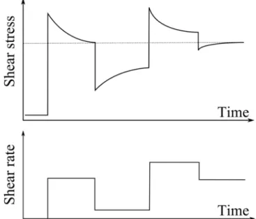
Structure changes during flow are generally studied within the frame of thixotropy. This typically concerns materials made of colloidal particles in suspension in a liquid and able to form weak links as a result of colloidal interactions(Mewis and Wagner [35]). The basic rheological trends of such a behavior (see Figure 2.8) are a viscosity decrease in time during flow or increasing shear rate and viscosity increase at rest or decreasing shear rate. It may be characterized with different rheometrical procedures (see Coussot [9]).The fundamental property in that context is reversibility: The flow structure may be broken but will anyway recover its initial characteristics after an appropriate flow history.

Figure 2.6. Material heterogeneities may create wall slip, where a thin fluid layer with lower viscosity forms between the wall and bulk fluid, giving the (macroscopic) impression that the bulk fluid has a

slipping velocity with respect to the solid wall.

Thixotropic characteristics also include overshoot stress at start-up experiments at constant shear rate, followed by stabilization to the steady state stress (Mewis and Wagner [35]). The flow history before each test matters. In creep tests where a sequence of constant stress steps is applied, the apparent viscosity may have a complex behavior, with different delay times to achieve very different steady state values (Coussot et al. [10]).

Figure 2.7. Fluids with unstable flow for an apparent shear rate below a critical shear rate _,, induce

heterogeneous velocity profile, as shear banding, creating an apparent flow curve.

Modeling such behaviors remains a very difficult task and a wide range of models have been suggested in literature (Coussot et al. [11]) but most of them contain a lot of parameters, which

(28)

have no obvious physical meaning or would need a long series of experimental tests to be measured.A similar situation is encountered in the field of waxy crude oil, i.e. various modeling approaches exist (see below), but the experimental data making it possible to fully check the validity of the models are even scarcer, in particular due to the difficulty to control at the same time the flow and temperature histories.

Figure 2.8. Typical thixotropic shear stress response to an imposed shear rate history.

The experimental approach of thixotropic behavior of usual concentrated colloidal systems is also complicated by the flow heterogeneities, such as shear-banding, which were shown to occur in Couette or cone-and-plate geometries (Ovarlez et al. [43], Pignon et al. [50], Møller et al. [38]).

2.3.3 Yield stress definitions

In the previous section, yield stress was presented as the minimum required stress by the fluid to flow. The fluid components may be arranged in certain way providing itself a structure capable of supporting external forces without continuous deformation. In fact, that is a very simple definition for a system that may exhibit complex solid-liquid transition when sheared beyond a critical deformation. That critical deformation corresponds to a critical stress, which also marks the transition from solid (or viscoelastic) regime to the liquid regime.

However, defining the yield stress also involves time-dependent effects. If a series of creep tests is performed, departing from the same material conditions, for shear stresses below the yield stress the material will increase its deformation with time until it stabilizes at a constant value. For shear stresses higher than the yield stress, the rate of deformation will increase until stabilizing in a constant strain rate. That kind of viscoelastic characteristic of the material may lead to long deformation equilibration times when the applied stress is close to the yield stress. Hence, it is time consuming to determine the yield stress experimentally by this method.

A faster but approximate method would be applying a shear stress or shear rate ramp. The beginning of the flow would be more difficult to define, as the material is deforming since the beginning of the test. If the imposed shear ramp is slow enough, a plateau may be observed in

(29)

the shear stress vs. shear rate curve. An alternative is to observe the decreasing ramp, looking for the minimum stress at which there was flow, just before the material comes to rest (when

→ 0). The special case of thixotropic fluids is discussed below.

Dynamic oscillatory tests may also be used to evaluate the yield stress. The oscillation amplitude can be increased with time and beyond a critical deformation the material viscous modulus should be higher than the elastic modulus. Below that critical deformation, the material would be in the solid regime, thus with higher elastic modulus. The oscillatory stress corresponding to the inversion between the moduli is said to be the yield stress. This is also a fast method for determining the yield stress, but submits the material to a complex deformation history.

Thixotropic fluids depend on the flow history, by definition. Thus, experimental procedures for determining its yield stress should take that characteristic into account, like the time at rest before the test and characteristic restructuring and destructuring times versus experiment duration. The shear rate or shear stress ramps, for example, should present a hysteresis between the increasing and decreasing ramps. In the increasing shear ramp the fluid presents a more structured state at the test beginning, thus presenting higher yield stress and apparent viscosity at the flow startup. As a result of the destructuring flow, the decreasing ramp may present lower apparent viscosity and the minimum stress to keep the flow should also be lower than the estimated yield stress from the increasing ramp. The yield stress determined from the increasing ramp is also called static yield stress and the yield stress from the decreasing ramp is the dynamic yield stress.

2.4 Macroscopic rheological behavior of waxy crude oils

2.4.1 General rheological characteristics

At temperatures above the WAT, the waxy crude oil has typically a Newtonian behavior. Its viscosity is independent of both shear rate and flow history and no yield stress is observed. At temperatures lower than the WAT, the wax crystals network is generally assumed to be at the origin of its non-Newtonian properties. According to Rønningsen [55] the oil exhibits a shear thinning behavior and a yield stress due to the existence of a network of bond linkages. It means that higher the shear rate imposed to the fluid, lower its viscosity, and for starting the flow, a minimum stress must be applied. Even if the yield stress concept may be questioned on a definition basis, for engineering applications it is a very useful concept and represents a reference number that fits well in the time scale of a pipeline restart and related field operations.

Rønningsen [55] also showed time-dependence behavior of waxy crude oils, indicated by a hysteresis loop during a stress ramp test, where the fluid is submitted to an increasing and then decreasing shear stress (this type of test will be discussed in details in Chapter 4). When the analyzed oil is sheared after being cooled at rest, the gel structure breaks down with time, reducing its yield stress and the hysteresis loop amplitude between the stress ramp cycles. So, the flow history has also a strong influence on the gelled oil rheological properties. Its instantaneous properties depend on the experienced flow.

That time-dependency recalls a thixotropic behavior, where the fluid apparent viscosity evolves in time due to the fluid structure changes. Though the classical concept of thixotropy states that

(30)

it is a reversible effect, Rønningsen [55] found that in some cases the recovery was not complete after having broken down the structure.

Thixotropic properties associated to structure breakdown and buildup were also described by Kané et al. [29]. Waxy oil structure buildup was also analyzed by Visintin et al. [77], who showed gel properties evolution while holding the fluid at rest at low temperature after different cooling rates and proposed a model for that evolution.

According to Lopes-da-Silva and Coutinho [32], the gel elastic modulus evolution during the holding time after cooling, which in their case lead to higher yield stress, is related to the gel structure development, where crystals reorganize or rearrange bonds.

In addition to those characteristics that may be observed at constant temperature below the WAT, the gel properties are affected by variations in the dynamic process of solids formations. As a result of solidification of some components in a multi-component fluid (as seen in section 2.2.1) and crystals aggregation, the gel properties are affected by the variables of that process. Namely, the solidification rate, whose kinetics is a result of the cooling rate and the shear forces imposed to the crystals during and after their formation. Many works indicate that the typical waxy oil behavior is the decrease of the gel strength with the cooling rate increase and shear rate increase while cooling, independently (Lin et al. [31], Lee et al. [30], Venkatesan et al. [71], Visintin et al. [77]).

The studies presented by Kané et al. [29] and Visintin et al. [77] provide clear evidences of that process dependency, showing that it is imperative to keep the proper tracking of the shear and thermal history of waxy oils to estimate its rheological properties.

Lin et al. [31] and Venkatesan et al. [71] revised studies with different conclusions on the gel properties regarding cooling rate and holding time after cooling. Some discrepancies in the behavior of those properties, as yield stress variations, may be attributed to impurities (Lin et al. [31]) and others to experiments procedures (Chang et al. [5], Venkatesan et al. [71]). Kané et al. [29] reported experiments with waxy oils with poor reproducibility and the possibility of having non-uniform shear at shear rates lower than 10 s-1 with cone-and-plate geometry. Dimitriou et al. [14] analyzed a waxy oil by Particle Image Velocimetry in a rheometer and found, for a steady imposed shear rate, fluctuating periods of flow with wall slip and structural erosion, breaking the oil gel progressively in smaller fragments. A comprehensive analysis of waxy crude oils sample preparation and possible sources of problems in rheological measurements can be found in Marchesini et al. [34].

Finally, the picture of a waxy crude oil cooling process may be rather complex: There is a solidification process, which has its own kinetics due to the different paraffin molecules; Then, forming a colloidal-type gel (Lopes-da-Silva and Coutinho [32]), where solids in suspension present interaction forces; In a fluid that may be in motion, with shear between different fluid layers, changing the solids relative position and the formation of aggregates. So, at the end of cooling and phase change, the system may still be out-of-equilibrium, letting place to structure rearrangements. Therefore, the resulting rheological behavior of the gel is function not only of the oil composition but of what happens during and after the cooling process.

(31)

2.4.2 Rheological models

2.4.2.1 Yielding model

The waxy oils yielding characteristics was investigated by Chang et al. [5]. They define three yield stresses to characterize the initial yielding of a waxy crude oil: τe, the elastic-limit yield stress,

below which the fluid exhibits a linear elastic response; τs, the static yield stress, the stress at the

starting point of immediate fracture or flow; And τd, the dynamic stress, an extrapolated shear

stress at zero shear rate obtained from the flow curve or from an instantaneous flow curve corresponding to a given sheared state.

According to the same authors, the creep condition, where yielding and plastic deformation start to occur, happens between the elastic and static yield stresses. It means that flow may occur at a shear stress below the static limit if sufficient time is given to the action of this imposed shear stress.

Chang et al. [5] and Chang et al. [6] present graphics of controlled stress and controlled shear tests in linear and log scale and also compare them with oscillatory tests, identifying the stresses limits in each graphic, as in Figure 2.9, for example. The fluid used was a waxy crude oil. All dynamic variables must be carefully controlled, to reduce the difficulty in measuring and defining those stresses in practice, as argued by Møller et al. [37].

(a) (b) (c)

Figure 2.9. (a) Difference between static and dynamic stresses in a controlled stress test at 16 °C; (b) stress vs. strain relationship in an oscillatory test at 20 °C and (c) storage, G', and loss, G", moduli.

Source: Chang et al. [5], p. 1552 and 1557.

Both the elastic and static yield stresses are dependent on the strength of the network of wax crystals in the oil, while the dynamic yield stress is related to the concentration, size and arrangement of the wax particles during the structure shear. It is important to note that the elastic and static stresses are highly dependent on thermal and shear history and on the stress loading rate. It implies that for direct application of those values on pipeline restart, the measurement must account for those histories.

For engineering proposes, the static yield stress is of most interest for determining the pump capabilities for restarting the gelled oil flow. Designing a pipeline restart based on the creep condition is considered nowadays much riskier. It would require high confidence in the fluid rheological model and a robust pipe flow model, properly relating the dynamic, creep and

(32)

compressibility effects for calculating the restart time and predict the behavior of the flow rate with time.

Several works in the literature were devoted to characterize waxy oils yield stress after different cooling histories. As said in the previous section, typically, lower cooling rates, lower shear rates and longer holding times at rest give rise to higher yield stresses, when analyzed independently (Venkatesan et al. [71], Lin et al. [31], Zhao et al. [83]). The oil-gel shear stress response at low deformations, as in creep and recovery tests, with the objective of analyzing its detailed yielding characteristics were also studied by Chang et al. [5], Kané et al. [29], Magda et al. [33] and Oh et al. [40], for example. More details on the yield stress measurement will be presented in Chapter 7.

2.4.2.2 Constitutive equations

Waxy crude oils below the WAT are described to be yield stress shear thinning fluids. A classical and efficient model for describing that type of fluid is the Herschel-Bulkley model. Indeed, the rheological behavior of waxy oils in steady state flow was already satisfactorily modeled using the Herschel-Bulkley model, but also Casson model, Cross model or Roberts-Barnes-Carew model (Rønningsen [55], Chang et al. [6], Dimitriou et al. [14] and Visintin et al. [77]). Those models are fitted on steady state flow data and represent the fluid rheological response in steady state to a certain flow and temperature history.

Transient models for representing the rheological behavior of waxy crude oils based on different strategies may be found in the literature. Generally, they were not specially developed for waxy crude oils, but inherited from other applications, as from food industry. Basically, three classes of models may be distinguished (Mewis and Wagner [35]): (1) The continuum mechanics approach, that introduce time-dependent function in existing models, as the Bingham model; (2) The microstructural models, that deduce macroscopic properties from the microscopic interactions between the material components and; (3) The structural kinetics models, where the fluid structure evolution is characterized by one parameter, that envelops the microstructural features, to be considered in the constitutive equation.

The first class of models was applied for waxy crude oils in, perhaps, its simplest way. The work of Rønningsen [55] used that strategy. In that work, Herschel-Bulkley and Casson models were fitted to waxy oils flow curves and a dumping function was used for reducing the rheological model parameters in order to account for destructuring flow. Later, Chang et al. [6] applied the same model for the flow restart of a pipeline with waxy crude oil, also treating the time evolution of the fluid apparent viscosity from results of viscosity decay experiments, where the apparent viscosity change was measured with time for various constant stress tests. Then for a given time of destructuring flow, one point of each constant stress test forms an “instantaneous” flow curve. Those various instantaneous flow curves were fitted by a time-dependent Bingham equation of the form:

+ / , for > , (2.3)

0 − ∞

1 + ) + ∞ (2.4)

The equations above describe one single flow and cooling history according to the experiments used to fit the parameters of the model. The function represents the yield stress while the

(33)

material is in the solid state, but in the liquid state it is only a mathematical fitting function of the instantaneous flow curve, without much physical meaning. It is similar to the curve parameter ₄ in Figure 2.9(a).

Dimitriou et al. [14] and Visintin et al. [77] presented similar approaches by fitting the strong variations of apparent viscosity in equilibrium states (steady state) obtained from imposed shear stress tests. That class of models has the advantage of directly fitting the oil rheological behavior. However, physical processes are let to a second plan, thus experiments must be very close to field conditions to which the model will be applied.

The second class of models, the microstructural one, relies on the physics of the interaction mechanisms of the material components. Such modeling approach, applied to waxy crude oils, based on fractal clusters, was proposed by Kané et al. [29]. They showed the thixotropic behavior of waxy oils during creep, recovery and transient imposed shear rate experiments. The common point with other classes of models is that they have also adjusted the unknown parameters of the model with the gelled oil flow curves (i.e. the apparent viscosity), but for different temperatures below the WAT. They have related those data to oil-gel structural observations of a previous work (Kané et al. [28]) in a fractal description of the media. One of the conclusions, however, stated that it was not entirely possible to relate the phenomenological parameters of the model for flow description with the structural features of the gel networks.

Considering the structural kinetic models, the third class, numerous models have appeared lately (see Mewis and Wagner [35]). However, few studies describe the flow evolution of waxy crude oils beyond yielding and its representation by pertinent rheological models. In literature this has been mostly done through modeling. A work of reference in that field is that of Houska [26] (applied in pipeline flow models by Sestak et al. [56], Cawkwell and Charles [4] and Wachs et al. [79]), who described the rheological behavior by a model in the range of classical thixotropic models for colloidal dispersions (see Coussot [9], Mewis and Wagner [35]). That model is the result of an evolution of representing thixotropic flows by generalizing the Bingham model. It includes a first equation, Eq. (2.5), of the Herschel-Bulkley type with yield stress and viscous coefficients depending on a structure parameter - 5, and a second (kinetic) equation, Eq. (2.6), describing the evolution of the structure parameter as a function of flow history, at constant temperature.

6 + 5 67+ ) + 5Δ) * (2.5)

85

8 9 1 − 5 − :5 ; (2.6)

In this description the yield stress can vary from a low value corresponding to a fully destructured fluid (5 0) to a high value for a fully structured material (5 1). The structure parameter evolves according to a kinetic equation with destructuring and restructuring terms. So a more structured fluid would have a higher yield stress and consistency coefficient, thus higher apparent viscosity. Under shear, the structure parameter reduces its value with time, representing a destructuration, thus reducing the yield stress and apparent viscosity.

The determination of the Houska model parameters is done by rheometry, exploring different shear values and structure parameter evolutions (see Cawkwell and Charles [4], Hénaut and