Commodity Price Shocks and Child Outcomes:
The 1990 Cocoa Crisis in Cote d’Ivoire
∗
Denis Cogneau
†R´emi Jedwab
‡May 28, 2010
Abstract
We look at the drastic cut of the administered cocoa producer price in 1990 Cˆote d’Ivoire and study to which extent cocoa producers’ children suffered from this severe aggregate shock in terms of school enrollment, labor, height stature and morbidity. Using pre-crisis (1985-88) and post-crisis (1993) data, we propose a difference-in-difference strategy to identify the causal effect of the cocoa shock on child outcomes, whereby we compare children of cocoa-producing households and children of other farmers living in the same district or the same village. This causal effect is shown to be rather strong for the four child outcomes we examine. Hence human capital investments are definitely procyclical in this context. We also argue that the difference-in-difference variations can be interpreted as private income effects, likely to derive from tight liquidity constraints.
Keywords: Education, Health, Child Labor, Commodity prices, Agriculture, Africa. JEL classification codes: I12, I21, 012
∗We thank the Ivorian National Institute for Statistics for giving us access to the surveys. We
also thank Michael Grimm, Marc Gurgand, Sylvie Lambert, Thomas Piketty, two anonymous reviewers and an associate editor for helpful discussions and suggestions, and seminar participants at Oxford (CSAE), London (Brunel and LSE), Stockholm, Clermont-Ferrand (CERDI), Madrid (Carlos III) and Paris (PSE and EUDN annual meeting). The usual disclaimer applies.
†Corresponding author. Paris School of Economics, IRD, DIAL. Paris School of Economics,
48 boulevard Jourdan - 75014 Paris. Tel: +33143136373. E-mail: cogneau@pse.ens.fr
Commodity Price Shocks and Child Outcomes:
The 1990 Cocoa Crisis in Cote d’Ivoire
May 28, 2010
1
Introduction
In many low-income countries and in Africa in particular, performances with regard to child health and education are still very disappointing. While the disease-prone environment and the low availability and quality of infrastructure bear a large re-sponsibility in this situation, on the demand side low parental resources constitute a direct limiting factor when liquidity constraints prevail. A large body of em-pirical research has already examined the multiple determinants of human capital investments in developing countries, like parental education, household resources or community resources, using structural production functions, reduced form ap-proaches, or a hybrid of the two (Strauss and Thomas 1995). This literature has long recognized the many econometric difficulties raised by the estimation of the causal effect of these determinants, because of the contamination of statistical cor-relations by unobservables stemming from other simultaneous household decisions (fertility, migration, labor supply), sample selection due to mortality, or endoge-nous programs’ placement. These difficulties apply in particular to the effect of parental income (see, e.g., Blau 1999); in that case, randomized experiments on conditional cash transfers are a recent answer (e.g., Schultz 2004; de Janvry et al. 2006; Filmer and Schady 2008). However, the impact of unconditional and
negative income variations are still not well known, and the African socioeconomic context is less studied.
Many recent works alternatively exploit the natural experiments generated by aggregate economic shocks: macroeconomic crises (Cutler et al. 2002; Thomas et al. 2004; Schady 2004; Pongou, Salomon and Ezzati 2006), commodity price changes (Edmonds and Pavcnik 2005; Kruger, 2007; Miller and Urdinola 2010), shocks on production (Jensen 2000; Yamano, Alderman and Christiansen 2005; Alderman, Hoddinot and Kinsey 2006; Maccini and Yang 2009) or targeted policy reforms (Duflo 2000; Edmonds 2006).
With those studies, the first issue at stake is sign identification: does a neg-ative aggregate shock increase or decrease investments in children? Indeed, as such a shock can reduce the opportunity cost of time for children and/or adults, children may work less and parents may have more time left for child care. This substitution effect may dominate the income effect and result in human capital investments being countercyclical. According to the survey made by Ferreira and Schady (2008), the income effect could however dominate in low-income countries, if only because of tight borrowing constraints. The few studies on African cases exhibit procyclical health and education: nutrition worsens and schooling is de-creased in times of drought or crop failure (Jensen 2000, for Cote d’Ivoire; Yamano et al. 2005, for Ethiopia; Alderman, Hoddinott and Kinsey 2006, for Zimbabwe). In contrast, in studies about Latin American countries, education often reveals countercyclical (e.g., Schady 2004, for Peru) whereas provided evidence is mixed in the case of health (procyclical: Cutler et al. 2002, for Mexico; countercyclical: Miller and Urdinola 2010, for Colombia).
A second issue lies in the interpretation of results. Reduced-form analyzes show that children are causally affected by shocks, but find it more difficult to disentangle the channels through which those shocks exert their impact, in con-trast with former contributions based on structural models (see, e.g., Jacoby and Skoufias 1997; Glewwe and Jacoby 2004). Indeed, depending on the context, many
determinants of human capital investments can vary concomitantly as a result of the shock, e.g. household income, health supply, education returns or child wages. Limitations in channel identification may arise from the nature of the shock under study, from data availability, or both. Still, in terms of policy, the attribution of these effects remains of outmost importance, for instance in the design of school fees or safety net schemes (Behrman and Knowles 1999; de Janvry et al. 2006).
Our strategy relies on the natural experiment provided by the unexpected and drastic cut of the administered cocoa producer price in 1990 Cote d’Ivoire. We exploit two datasets from nationally representative large sample household surveys that were implemented before and after the cocoa crisis, in 1985-88 and 1993 respectively. First, we show that the cocoa crisis did negatively affect the human capital of cocoa producers’ children by comparing them with non-cocoa farmers’ children, across time, within the same geographical area, and along several dimensions: school enrollment, child labor, height stature, and illness incidence. Human capital investments reveal procyclical in this context. Second, we argue that the cocoa crisis did not affect child outcomes through any important channel other than household income.
The remainder of this paper is organized as follows. Section 2 presents the historical background, the data, our difference-in-difference identification strate-gies, and the main reduced-form results. Section 3 discusses the biases that may affect the estimates of the impact of the cocoa price shock. Section 4 discusses channels of transmission, then examines results in detail and argues that the pri-vate income effect should dominate over price effects. Section 5 concludes.
2
Background, Data and Identification
2.1 Background
From independence till the 1980’s, Cote d’Ivoire has experienced dramatic growth thanks to the development of cocoa exports. Cocoa being produced by
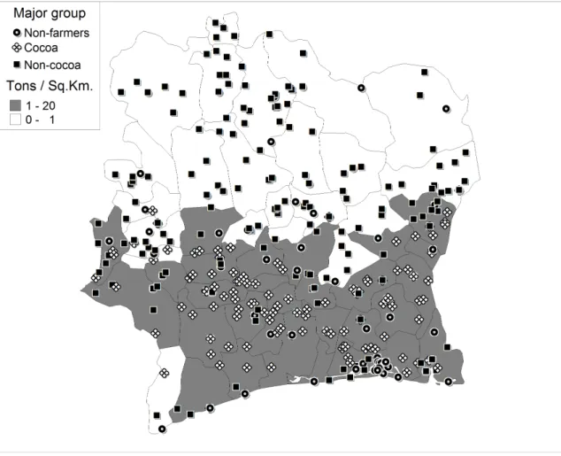
replac-ing forest trees with cocoa trees, its production is limited to the Southern (and forested) half of the country. Coffee is also grown in the forest regions, although to much lower volumes, and about two-thirds of coffee producers are also cocoa producers. The Northern Savannah region does not produce cocoa at all and grows instead cotton as an export crop. Figure 1 displays a map of Cote d’Ivoire, where administrative districts (”d´epartements”) and survey clusters (primary sampling units) have been categorized according to the importance of cocoa production.
[ Insert Figure 1 about here ]
The cocoa producer price was administered by the state-owned marketing board (the ”Caisse de Stabilisation et de Soutien des Prix des Produits Agricoles” -CSSPPA or ”Caisstab”), which fixed it below the international price. The Caisstab never played its role of international prices stabilization and served as an implicit taxation of agriculture. From 1979, the decline in the international cocoa price and the increasing deficits of the Caisstab forced the government to cut the producer price for the first time in 25 years, first from 400 to 250 CFA francs per kilogram in June 1989, and then to 200 CFA Francs in 1990 (see figure 2).
[ Insert Figure 2 about here ]
The administered coffee price had already been cut from 385 to 200 CFAF in 1985 and remained stable thereafter. As regards other agricultural productions, the administered cotton price only fell from 115 to 90 CFAF between 1988 and 1993, and (non-administered) staple food prices also decreased but to a much lesser extent (between 20 and 30 percents) than the price of cocoa (Jones and Ye 1997, p.11-12). 1985 to 1988 have been years of high yields and high prices for cocoa producers, and yields remained high after 1990 (Jones and Ye 1997, p.7).
Given these evolutions, between 1988 and 1993 we expect the income of districts producing cocoa to have fallen more than the income of other districts.
Likewise, within cocoa-producing districts, we expect the income of farmers who grow cocoa to have fallen more than the one of other farmers. This is confirmed by figure 2: whereas cocoa-producing households exhibit a 20% higher level of consumption per capita in 1985-88, they end up at par with other farmers in 1993. 2.2 Data and Variables
Our main sources of data are the four Cote d’Ivoire Living Standards Measurement Surveys (CILSS) from 1985 to 1988, and the Enquˆete Prioritaire (EP) 1993, all conducted by the Institut National de la Statistique of Cote d’Ivoire with the support of the World Bank. Although the 1985-88 surveys include a small two-years rotating panel (for less than half of the sample), we do not make use of this dimension. The 1993 survey is a completely independent sample. Not having a panel running across the pre-shock and post-shock periods (in contrast with Thomas et al., 2004, for instance) raises important identification difficulties that we try to address later on. As we are mainly interested in the comparison of children between the pre-crisis and the post-crisis period, we stack all the household data for 1985-1988. In the end, when looking at the population of 0 (more than 6 months) to 15 year-old children, we obtain 22,811 individuals in 5,299 households across 200 primary sampling units (PSUs) or survey clusters in 1985-88; and 26,977 individuals in 7,358 households across 480 PSUs in 1993.1
We are able to isolate sub-samples of children whose living conditions de-pended the most on cocoa production and income. First, we can define in an homogeneous way across surveys the group of cocoa-producing households among farming households, whether they are landowners with tenants who grow cocoa trees, or landowners or sharecroppers who directly grow cocoa, provided that more than 1 kilogram of cocoa beans were harvested. Hence we can divide the sample
1As explained in the surveys’ documents, the 1985 and 1986 samples were biased in that they
over-represented large size households, but an ex-post sample reweighing corrects for this bias. All our estimates use the probabilistic sample weights with this ex-post correction.
into three occupational groups: cocoa-producing farmers, non-cocoa farmers, and non-farmers. As we shall see later on, the shares of those three groups varied little across the cocoa crisis. Second, the district of birth of each child is reported, based on an administrative grid that distinguishes 50 districts;2 hence we can also break down our children samples according to the density of cocoa production in the dis-trict of birth, using administrative (hence survey-independent) cocoa production data for the pre-crisis period (1985-88). Among these 50 districts, we isolate the 28 southern districts where this density of production is higher than one ton of cocoa beans per squared kilometers (see figure 1 above).
[ Insert Table 1 about here ]
We consider four child outcomes. Table 1 provides some descriptive statistics for children living in agricultural households, broken down by gender and period. Regarding school enrollment, we distinguish two age groups, 6-11 and 12-15, 11 being the theoretical age of completion of primary school. The surveys do not provide information on other outcomes such as age of entry into school or curriculum, and literacy is not asked the same way in both surveys. With current enrollment, the month of interview is an issue: for instance, enrollment is under-reported in August as it is a period of holidays. We instead use ”currently enrolled
or enrolled in last 12 months”, that does not exhibit a significant seasonality.
Regarding child labor, we have information on work in the last 7 days and the last 12 months for individuals over 7 years of age. In contrast with school en-rollment, choosing the 12 months reference period does not cancel out seasonality: children are still declared more often at work when interviewed during the spring season. This points out that child labor is subject to strong recall bias. We hence privilege the last week reference period. We assess the robustness of our estimates to the inclusion of month of interview controls, and also check that the 12 months
2The 1985 survey makes an exception, as the grid that prevailed before 1986 only distinguished
reference period provides the same qualitative results. In table 1, the observed decline of child labor between 1985-88 and 1993 partly stems from the fact that the 1993 survey does not include the spring season where child labor is maximal. We have no reason to believe that work on the farm reporting varies with the spe-cialization of households, i.e. whether they produce cocoa or not (and even more so when we compare farming households within the same district or the same vil-lage as we do in our preferred estimations thereafter). We hence consider that our difference-in-difference strategy successfully cancels out any remaining difference in child labor reporting between the pre-crisis and the post-crisis periods.
Turning to health outcomes, height stature is measured in each survey for children between 6 months and 4 years (59 months) of age. For age in months, heaped or missing values are observed as in many surveys. We construct two types of height-for-age Z-scores using the World Health Organization standards (WHO 2006): observations with missing age in months are given their age in years times twelve plus six, or else times twelve; we also analyze height regressions with controls for sex and age in years and their interactions. We primarily use the first version of Z-scores, and use the other two for robustness checks. For reasons discussed later, we are led to distinguish two sub-samples: children from 6 to 23 months (all of them being born after the shock) and children from 2 to 4 years.
Last, parents declare whether their child has suffered from an illness or an injury during a reference period preceding the interview; the question is exactly the same in both surveys, except that the reference period is the past four weeks in the 1985-88 surveys and the past two weeks in the 1993 survey. For analyzing this incidence of morbidity, we consider two sub-samples of children: 6 months to 5 years and 6 to 15 years. The halving of the reference period explains why morbidity has decreased between 1988 and 1993. Our difference-in-difference strategy should adequately correct for this definitional change.
Our income variable is consumption per capita (at 1988 prices), since con-sumption is better measured than income in poor countries. We are careful to
include the consumption of own food production and imputed housing rent, and to exclude very infrequent durable goods acquisition and health expenditure. In-come available for consumption corresponds to the ex-post inIn-come once coping strategies have been implemented to mitigate the ex-ante cocoa income cut: in-crease in labor, dissaving and sale of assets, borrowing, etc. For the whole sample, we estimate real per capita consumption to have fallen by 39% between 1988 and 1993, which is not completely inconsistent with estimates from Maddison (2003) indicating a 27% fall of real GDP per capita. The survey figure is the same for the population of 0-15 year-old children in agricultural households (see bottom line of Table 1), with consumption per capita falling from 436 to 265 CFA francs (at 1988 prices), i.e. a 39% drop again.
Finally, both surveys allow us to gather a large set of control variables, regard-ing the household demographic composition and assets, and child and household head characteristics. Those variables are reviewed when used in section 3.
2.3 Difference-in-Difference Identification Strategies
As already stated above, we define a first (and preferred) treatment group, the sample of children living in cocoa-producing households, and contrast it with the sample of children living in non-cocoa farming households. Figure 2 confirms that mean consumption per capita has fallen more for cocoa households than for their non-cocoa counterparts, by 45 against 33 percents, although each category has been very much affected by the cocoa-induced macroeconomic crisis.
Alternatively, we define a second treatment group, the sample of children born
in cocoa-producing districts, and a comparison group, the sample of children born in non-cocoa districts (defined as producing less than one ton of cocoa per square
km in 1985-88). When referred to the literature, this district-level strategy echoes the exploitation of rainfall shocks (Jensen 2000; Maccini and Yang 2009), or price shocks when data on household-level specialization is not available (Kruger 2007; Miller and Urdinola 2010). Consumption per capita evolutions are very close to
those obtained with the first cocoa/non-cocoa categories: a 41 fall against a 31 percents fall, even if here non-farmers contribute to the comparison.
We look at the dynamic relationship between cocoa specialization and house-hold income by estimating the following difference-in-difference regression model:
Sivt= αCocoaivt+ βCocoa1993,ivt+ Xivtγ + Vvt+ uivt (1)
For each child i observed in area v at year t (t = 1985, 1986, 1987, 1988, 1993), Sivt
is the outcome under consideration. This specification will be the same for all the reduced-form estimations that will be implemented in the remainder of the paper, whether for household income, child outcomes or other household level or child level variables. Cocoa is a dummy variable indicating whether the child belongs to the ”cocoa” treatment group, i.e., depending on the regressions, belongs to a cocoa-producing household or is born in a cocoa-producing district. Cocoa1993 interacts Cocoa with a dummy for the year 1993. X is a set of control variables, including a constant and a time dummy for the year 1993; other variables like the date of interview can be introduced for robustness checks. For regressions involving our preferred treatment group (Cocoa defined from household-level production), the district and village (survey cluster) fixed effects specifications include a set of dummies for the area of residence interacted with year, in order to control for all factors common to children living in the same area in the same year (Vvt). In all
household level estimations, standard errors are clustered at the level of primary sample units (PSUs), i.e. survey clusters. When district of birth level estimates are considered, standard errors are clustered at the same level, i.e district of birth-year, so as to avoid over-optimistic inference with differences-in-differences (Bertrand, Duflo and Mullainathan 2004).
2.4 Main Results: a Preliminary Overview
We first estimate regressions with log per capita consumption on the left-hand side, for the sample of 0-15 year-old children. The coefficients of Cocoa1993 are reported in panel A of table 2. They show that the crisis was associated with
a relative income loss for cocoa-producing households, ranging between 8 and 15 percents depending on the specification. We then run the same regression for human capital outcomes. Panels B to E of table 2 present our preferred reduced-form results for specific age ranges; more details about this selection are given in section 4. These results show that in 1993 the situation of ”cocoa children” has significantly deteriorated in comparison with others: the 6-15 year-old are less often enrolled at school (panel B), the 12-15 year-old are more often working (panel C), the 2-4 year-old are relatively shorter (panel D) and the 6-15 year-old are more often declared ill or injured (panel E). We already notice that while estimates based on cocoa production at the district of birth level (last column) are pretty much in line with those based on cocoa production at the household level, they are less precise as they exploit a limited source of variability (50 districts).
[ Insert Table 2 about here ]
Our reduced-form results indicate that human capital is procyclical in this context, and are in keeping with some other works on Africa already reviewed in the introduction. Our two figures about schooling and stunting suggest that the cocoa price shock might have had serious consequences on the ”capabilities” of the children living in cocoa-producing households. It is possible that some minimal education was not received and could not be recovered; the same holds for the small stature inherited from stunting in that it reflects an irreversibly diminished health capital. Taking these results as only preliminary and suggestive, we now examine whether our difference-in-difference strategy is well-founded.
3
Potential Bias of the Difference-in-Difference Strategy
First, we must assess whether we have any indication of exogenous differential trends between our treatment and comparison groups that could account for the evolutions observed. Second, we must check that endogenous composition and selection biases do not contaminate our comparisons across time.
3.1 Pre-Shock Trends
We take advantage of the four-surveys structure of our pre-shock data, and use the date of interview (month-year) to control for monthly pre-shock differential trends. The four pre-crisis surveys cover a period running from February 1985 to April 1989, hence two months before the cocoa price shock which occurred in June 1989. We run the same model as in equation (1) except that we include one trend variable T (number of months since February 1985) and its interaction with the cocoa dummy, Cocoa × T . Observations of the 1993 post-crisis survey are set at the forecasted June 1989 value.3
S = α0Cocoa + β0Cocoa1993+ Xγ0+ δ0T + θ0Cocoa × T + V0+ u0 (2) Estimating both models with the seemingly uncorrelated residuals (SUR) method, we then test whether the Cocoa1993 dummy coefficient in the augmented model (2) is significantly different from the estimate obtained in the basic specifi-cation (1), i.e. H0 : β = β0. As month of interview variation within each survey
partly reflects the phasing of sample designs across space (indeed, district-year fixed effects explain about half of month of interview variance, and village-year fixed effects more than 90%), we also check that the same results are obtained when replacing the month of interview trends by year of interview trends. For the five outcomes already studied in table 2 and for the ”pooled” specification, the full set of estimates of this augmented model are displayed in the top panel of table 3. The bottom panel reports the Cocoa1993 coefficient obtained for the other specifications.
[ Insert Table 3 about here ]
3We could have alternatively set them at the June 1993 value, assuming that pre-shock trends
are valid forecasts for the 1989-93 period; as we shall see, such an heroic assumption would lead to an even bigger impact of the cocoa shock.
In the top panel, the third line shows that there is no significant pre-shock trend for cocoa producers relatively to non-cocoa producers (i.e. θ0 = 0). The fifth
line and the corresponding SUR χ2tests suggest that introducing pre-shock trends brings little change to the difference-in-difference evaluation of the impact of the shock. In all cases, the impact of the shock on cocoa children is even enhanced as pre-shock trends are taken into account, especially for consumption per capita and child labor, although not significantly so. The same results hold for the other specifications. With district or village fixed effects, the shock on consumption per capita is only estimated to be significantly larger than in table 2, with a fall of around 18-20% against 8-10% when pre-shock trends are not introduced. If anything, considering pre-shock trends would finally lead us to re-estimate upward the impact of the shock, as during the years preceding the shock the cocoa children living standards were slightly improving relative to others.
3.2 Composition and Selection Biases
We study whether other factors than the price and income shocks have influenced the observed difference-in-difference in outcomes between ”cocoa children” and their non-cocoa counterparts. This caution is most important for the estimates based on household-level specialization, as the crisis may have affected the stability (in terms of observables and unobservables) of both our treatment and comparison groups. In contrast, the district of birth level estimates should rule out this kind of bias: for children of at least 2 years of age born before 1993, the district of birth is predetermined before the cocoa price crisis, provided that the price shock was not anticipated. The fact that these latter estimates, although more imprecise, provide similar figures as household level ones (see tables 2 and 3) can already be considered as pretty reassuring. Conversely, and in contrast with the district-year or village-year fixed effects versions, the district of birth approach does not discard price effects going through local public goods provision or local labor and product markets. But this latter aspect does not question the reliability of the
difference-in-difference, but has to do with the channels of transmission of the shock and is examined thereafter in section 4.
3.2.1 Occupational Mobility
We first observe that the shares of cocoa and non-cocoa households in the total population kept relatively stable between 1988 and 1993: respectively 27.5 and 29.2 for cocoa producing households, 38.7 and 37.1 for non-cocoa agricultural households. This means that within the farming households sample, the share of cocoa-producing households increases from 41.5 to 44.0. This latter share is even more stable when restricting the sample to districts (resp. villages) where at least one cocoa farmer and one non-cocoa farmer are observed: 50.7 (resp. 56.6) to 51.3 (resp. 57.1); those latter sub-samples are the ones used for the identification of the district-year FE and village-year FE models. We also calculate the share of cocoa households in each village and check that the density distribution of this share did not change between the two years. At the aggregate level, we are confident that our two groups exhibit a great deal of stability. This aggregate stability should already limit the potential for selective mobility in or out these two sectors.
Furthermore, for households who were already in the cocoa sector before the crisis, it is unlikely that they have given up cocoa, as growing cocoa imposes irreversible investments. A cocoa tree needs 5 years to produce cocoa beans, is mature after 10 years, and may live much longer. A specialist of this sector even noticed some ”optimism from cocoa producers” at that time, resulting from several factors (Ruf 1995, p.191). First, they had no alternative as profitable as cocoa. Second, they were expecting a price upturn, which indeed happened as soon as in 1994. This optimism is confirmed by the fact that many cocoa trees were still being planted at that time. National statistics show that cocoa production and the total area devoted to it did not significantly change between 1988 and 1993. In the case of neighboring Ghana, Hattink, Heerink and Thijssen (1998) review price elasticities estimates for cocoa production from aggregate time series data and
provide their own using farm-level data: altogether estimated short-run elasticities range from 0.13 to 0.29; they conclude that price variations have a small effect on resource allocation for cocoa production in the short run. We thus consider that the vast majority of cocoa farmers of 1988 were still in place in 1993, even if they may have further diversified their activities. Yet, these aggregate features do not preclude more subtle compositional changes at the margin, stemming for instance from the differential characteristics of new entrants in each sector. This is what we examine thereafter.
3.2.2 Relative Changes in Observables
In order to test for the compositional differences between cocoa and non-cocoa households, we look at the set of variables that can be gathered in the surveys and regress each one of them as in equation (1) for the sample of 0-15 year-old children. The coefficients of Cocoa1993 are reported in table 4 for a subset of these variables and for the three household level models. If we take the within-district differences as a benchmark, in the pre-crisis period, the two groups not only differ in mean income levels but also in household size (2 additional members on average in cocoa households) and livestock wealth (10 percentage points more livestock owners); besides, the heads of cocoa households are more often men, uneducated, non-migrants and are older by 2 years. But a difference of mean characteristics between groups is a source of bias if and only if it varies over time.
No significant changes are observed in the case of the district-year fixed effects specification (middle column of table 4). The only significant differential changes we could spot are : (i) a decrease in both the shares of female heads (by 3 percentage points) and of educated heads (by 7 points) in cocoa households, when compared to the pooled sample of other farmers (when no spatial fixed effects are introduced); (ii) the household head ageing by 3.5 years in cocoa households, when compared to their village neighbors (village-year fixed effects estimates). Part of the pooled differential changes stem from non-cocoa farmers located in
northern areas where cocoa is not produced. When restricting the comparison to districts where at least one cocoa farmer is observed, the educational difference mentioned above vanishes. The head’s differential ageing in cocoa households might be explained by the easier absorption of young households by the non-cocoa sector where entry requires more investments. This investment constraint could be even more binding in time of crisis. However this mechanism should hold as well for the pooled or the district FE comparisons, whereas it does not significantly so. We rather conclude for some sample variation. It is the case that when keeping only the 1985-86 pre-shock years, this differential ageing is no longer observed. As the head’s age may still influence some of the four outcomes, we include it as a control variable and check that our point estimates are not altered.
[ Insert Table 4 about here ]
3.2.3 Selective Fostering and Endogenous Fertility or Mortality
Cocoa households could have fostered less children in 1993 than in 1988, when compared to non-cocoa households. The 1985-88 surveys contain a specific section dedicated to fostered children, from which we learn that, among 2-15 year-old chil-dren, about 1 child out of 4 is fostered and that children are around 5 percentage points more likely to be fostered when they belong to cocoa-households. However, this small difference no longer holds when spatial fixed effects are included. Yet, there is no data on fostered children in the 1993 survey, and our identification strat-egy could be contaminated by some endogenous variation across time of household composition. We examine whether the relative probability to be born outside the district of residence varies over time, which could indicate between-district foster-ing. We also check whether the likelihood of being the head’s biological child varies across time with belonging to a cocoa household. Table 4 confirms that if a change has occurred, it was a very slight and non-significant one: see the coefficients of
Besides, the crisis could have increased child mortality relatively more for cocoa households and/or induced those same families to postpone their fertility decisions, which would lead to an endogenous change in the number of young children between cocoa-producing and non-cocoa farming households. In the first line of table 4, we examine this possibility by looking at the probability of having a child between 6 and 23 months of age among the sample of 0-15 year-old children. It is indeed in the former age range that we expect child mortality to be the highest; besides, children less than 2 years of age have all been conceived after the shock was observed. We also try with other age ranges (0-3, 1-4, 2-4), and we also test with other comparison groups: 6-15, 6-11, 12-15. In the end, the coefficient of Cocoa1993 is always close to 0 and non-significant, suggesting that there is no differential variation in mortality or fertility between our treatment and control groups.
In the end, the examination of potential biases leads us to grant our prefer-ence to the district-year and village-year fixed effects estimates, which show the greatest stability in both the demographic weight and the relative composition of the population of cocoa children compared to non-cocoa children. Furthermore, as we discuss immediately thereafter, interpretation of the differences-in-differences is made easier when controlling for common factors shared by cocoa and non-cocoa households living in the same area.
4
Detailed Results
We now expand on the basic results provided in table 2, for our preferred district or village fixed effects estimates. We begin by discussing the price and income effects that could plausibly take place as a consequence of the shock.
4.1 Price and Income Effects
The cocoa price shock had the obvious consequence of tightening the budget constraint of the great majority of Cote d’Ivoire households, and even more so for
cocoa-producing households. Additionally, the cocoa crisis could have modified the prices and costs, whether explicit or implicit, that are relevant when parents decide to invest in their children, and again differentially so for cocoa producers. We investigate each one of these price channels, and argue that the income effect dominates the results, at least once spatial fixed effects are introduced.
4.1.1 Local Supply and Interactions
We expect the aggregate income of villages with more cocoa farmers to have decreased more. If the provision of public goods like schools and health centers is partly determined at the local level, we expect a relative decrease in the quantity and/or the quality of human capital supply, hence a relative rise in the cost and shadow price of human capital investments for cocoa farmers. Likewise, a local variation of child and adult wages influence household labor supply, time allocation, and human capital decisions. Non-market social interactions also play a role: as some selected families withdraw their children from school or delay their entry, other neighboring families can be induced to do the same. However, when including district and even village-year fixed effects, we are controlling for all these channels whose effects are shared by households living in the same area. The inclusion of those fixed effects implies that the only price changes which matter are those affecting differentially the human capital investment decisions of cocoa and non-cocoa farmers living in the same local environment.
4.1.2 Returns to Education
As the cocoa price falls, the expected returns to education could decrease more for cocoa producers than for non-cocoa farmers, even within the same village. This is true as long as cocoa producers invest in education so that their children be cocoa producers, and as long as they expect the price shock to be sustained. However, as already mentioned before, cocoa producers remained rather optimistic about the cocoa price prospects. Furthermore, cocoa production is not particularly intensive in human capital. The surveys tells that heads of cocoa households are
actually a bit less educated than other farmers. Education is better seen as a strategy to allow children to escape from the agricultural sector or to diversify production activities, so that cocoa and non-cocoa farmers should share the same expected returns to education, especially when they live in the same area.
4.1.3 Time Allocation
As the cocoa price falls relative to other export and food crops, both child and adult labor become less profitable in the cocoa sector. With imperfect local labor markets, the child and adult opportunity costs may be different in cocoa households compared to non-cocoa households. Cocoa-farmers might then real-locate more labor to other activities and/or reduce more labor supply. In this latter case, a price-induced decrease in child labor could be indirectly beneficial in terms of school attendance and health status; likewise, a price-induced increase in adult leisure could bring more time for child care in cocoa households (e.g., Miller and Urdinola 2010). We do not believe that these substitution effects carry an important weight in our context. First, we already noticed above that national cocoa production has not changed much over the period. Second, the observed reduced-form impacts of the crisis on child labor is either positive or null, not negative: on average, older children (12-15 y.o.) of cocoa households significantly increase their labor participation (panel C, table 1) while the youngest (7-11 y.o.) do not (see table 5 thereafter). Indeed, households mainly use child labor as in-surance (e.g., Jacoby and Skoufias, 1997). Third, we implement the same test for adult labor, by estimating equation (1) for 18-60 year-old individuals. The 1993 survey does not provide for the hours worked either by children or adults, so that our analysis is confined to the discrete decision of labor participation. We detect no significant variation in adult participation in the district or village FE speci-fications, and rather a slight increase in the pooled estimates. Then, even if the relative price decrease has a substitution effect on time allocation, it is very much counterbalanced by the income effect which plays in the opposite direction.
4.1.4 Income Effect
In the end, we believe that our differences-in-differences estimates with spa-tial fixed effects capture a true income effect, like the one that would be observed in a virtual field experiment whereby a significant amount of income would be unconditionally withdrawn from the pockets of randomly selected households. Al-though we cannot definitively prove it, we believe that this income effect mainly goes through the liquidity constraint channel: when confronted to an income short-age, families are unable to pay for more or better food, schooling or health costs, whatever the coping strategies they implement (including child labor).
We now turn to a more detailed and disaggregated description of the im-pacts of the shock. Under our argument that the private liquidity constraint is overwhelming, tentative IV estimates of the income elasticities of child investments may be computed. They are mainly meant to provide a money-metric benchmark for the comparison with other shocks examined in the literature, having different magnitudes and taking place in different contexts.
4.2 School Enrollment and Child Labor
Table 2 suggests that the local context plays an important role in school enroll-ment and child labor (panels B and C): the estimates of the impact of the cocoa shock with district or village fixed effects are significantly lower than in the pooled specification. We have no way of disentangling the various local effects that may account for that result, whether they stem from relative prices evolutions, labor markets, public goods provision or social interactions. However, the fact that dis-trict FE estimates are not very different from village FE suggests that non-market interactions among close neighbors are less involved than other factors.
According to table 2, the cocoa price shock has decreased the school en-rollment of 6-15 year-old cocoa children by 5 percentage points on average with district FE, and the same with village FE. If we assume that all this variation can be attributed to a private income effect, we may compute the double least
square estimates for the corresponding income elasticity; we obtain a rather large 0.60 elasticity in the former case (district FE) and 0.43 in the latter (cluster FE).4 These IV estimates reach about four times the value of the OLS estimates, point-ing out the existence of strong downward biases affectpoint-ing the correlation between income and school enrollment. The same thing is found for 12-15 year-old child labor; this latter result suggests that simultaneity of income and labor decisions play a minor role, as simultaneity should here generate an upward bias.
Our computations of the school enrollment income elasticity show the same orders of magnitude as previous results in the literature. In a completely different context (i.e. ten villages of semi-arid India between 1975 and 1978), and with panel data estimation including village-season-year dummies, Jacoby and Skoufias (1997) get a 0.32 for the income elasticity of school attendance of 5 to 18 year-old children. Likewise, looking at the school enrollment of 10-18 year-old Vietnamese children between 1993 and 1998, Glewwe and Jacoby (2004) recover income elas-ticity estimates ranging between 0.20 and 0.40. Much closer to our case, Jensen (2000) studies the changes in enrollment experienced by children in Cote d’Ivoire between 1986 and 1987, using the same surveys as our pre-crisis set. He distin-guishes children living in regions hit by an adverse rainfall shock. He finds that enrollment rates declined by 20 percentage points for 7-15 year-old children in shock regions relative to children in non-shock regions; relative income per capita falls by around 30 percents, so that the enrollment figure corresponds to a Wald estimate of income elasticity of about 0.66.
[ Insert Table 5 about here ]
Yet, our aggregate estimates can be misleading if they uncover heterogenous responses. In table 5 we distinguish boys and girls as well as three age sub-groups (6-8, 9-11, and 12-15), and estimate the reduced-form model with sex and age
4IV estimators were calculated using the Stata module Xtivreg2 (Schaffer 2007). Hausman,
interactions added. This breakdown of the average decrease in enrollment tells us that girls are much more affected than boys before age 11, while boys are much more affected than girls after age 12. As regards labor, all the impact of the cocoa shock is concentrated on boys between 12 and 15 years of age. Younger kids and girls aged 12-15 seem completely unaffected, even if for the latter it must be remembered that household chores are not included in our child labor variable. In the absence of panel data, we have no direct way of identifying whether the decline in school enrollment is due to delayed entries or dropouts, and whether children who are put to work are withdrawn from school. We can only presume that the enrollment of younger girls is most probably delayed, whereas already enrolled girls who are closer to the age of marriage are kept at school; as described by Bommier and Lambert (2000) on the case of Tanzania, this parental behavior should in any case result in a shortened school curriculum for younger girls as a result of the crisis. As for boys, while their school enrollment is more protected at lower ages, the increased use of their labor at later ages could have directly resulted in reduced schooling. However, the extent of this latter reduction in enrollment does not fit one-to-one with the increase in labor, and does not close the gap with girls which stays as large as 16 percentage points within 1993 cocoa households.
4.3 Height Stature and Illness
Here the local context is less binding, as the comparison of pooled and fixed effects estimates in table 2 can tell. Children between 2 and 4 years of age living in co-coa households have lost between 0.3 and 0.6 international standard deviations in height-for-age, when compared to children of other farmers. This impact is rather large. It is robust to an alternative imputation of missing age in months, and is also maintained when height is directly analyzed with sex and age in years con-trols. Table 5 indicates that young girls are more affected than boys. Being more short-term oriented, other anthropometric indicators like weight-for-age, height-for-weight or body mass index, do not reveal any significant impact. The impact
of the cocoa shock is not visible on children aged from 6 to 23 months either, whichever specification is chosen. This however does not mean that those younger children did not reveal stunted later on. We have indeed good reasons to think that the scarring effect of the shock could be blurred in this population. First, the potential impact of errors on date of birth is certainly greater before two years of age because growth in stature is maximal between 0 and 23 months. Second, nutri-tional differences are better revealed at childhood stage (ages 2-4), when children are no longer breastfed and height velocity stabilizes (see Bogin 1999, pp.67-79; Moradi 2006). Third, as we are studying a persistent income shock, the duration of exposure to bad living standards can matter. The great majority of the 2-4 year-old children have been exposed to the cocoa shock since birth; hence we can say nothing about the timing of the scarring effect, in contrast with Maccini and Yang (2009) who relate rainfalls in the year of birth to height stature at adult age. As our result holds with village fixed effects, it cannot be attributed to changes in the infectious environment, but rather to lack of health care and to worsened nutritional conditions. The income shock directly affects the drugs or food that households can afford to buy, and the increase in the work effort of other members, like 12-15 year-old brothers, may require more food intakes that compete with the food left available to the youngest.
Turning to our last outcome, estimates of table 2 and of table 5 all confirm the increased incidence of morbidity among 6-15 year-old cocoa children compared to their non-cocoa counterparts: cocoa children are more often declared ill or injured by 3 to 4 percentage points, and this impact is well-balanced between genders. We could have thought that the heavier workload of 12-15 year-old boys would have a direct influence on their morbidity, if only through an increased exposure to wounds or injuries; but this is not what we find. Besides, we do not find any increase in morbidity incidence among younger children aged from 6 months to 5 years. As younger children are about twice more often declared ill (see table 1), this absence of impact may be attributed to the coarseness of our discrete
indicator, whereas a continuous variable like height-for-age Z-score is more able to capture the deterioration of health conditions at early ages. It is striking to observe that the naive correlation of this variable with household income is positive, as is often found with health self-assessments: rich parents are more able to recognize symptoms and over-report that their children are ill, whereas poor parents lack knowledge about illness or are more used to suffering and under-report. With our difference-in-difference strategy, this spurious source of correlation is canceled out.
5
Conclusion
We look at the drastic cut of the administered cocoa producer price in 1990 Cote d’Ivoire and study to which extent cocoa producers’ children suffered from this severe aggregate shock in terms of school enrollment, labor, height stature and morbidity. Using pre-crisis (1985-88) and post-crisis (1993) data, we propose a difference-in-difference strategy to identify the causal effect of the cocoa shock on child outcomes, whereby we compare children of cocoa-producing households and children of other farmers living in the same district or the same village. This causal effect is shown to be rather strong for the four child outcomes we examine. Hence human capital investments are definitely procyclical in this context. We also argue that the difference-in-difference variations can be interpreted as private income effects, likely to derive from tight liquidity constraints: parents would like to invest in their children but cannot afford to. African economies remain little diversified and vulnerable to changing international prices for their exports. In Cote d’Ivoire, a considerable part of the population still directly suffers from the fluctuations of those prices. In the past, the national marketing board and price stabilization fund for cocoa, the Caisstab, did not really served its original mission; it was dismantled in 1998. Nevertheless, new insurance schemes and safety nets could be invented to protect households and children from unexpected negative income shocks. If one believes the estimates presented here, those programs might constitute a defendable use of foreign aid money.
Figure 1: District Density of Cocoa Production and Main Occupation of Survey Villages
Note: District density of cocoa production is calculated as district production of cocoa beans in tons (1985-1986-1987-1988 average) divided by district area in squared kilometers. Sources: CSSPPA (1990) and author’s calculations. Circles, lozenges and squares are primary sampling units (PSUs), i.e. survey clusters. An occupa-tional group = {non-farmers, cocoa (farmers), non-cocoa (farmers)} is defined as the major group in the PSU if it gathers the highest number of households. Sources: 1985-88 and 1993 household surveys, authors’ calculations.
Figure 2: Cocoa Producer Price and Mean Per Capita Consumption of Cocoa and Non-Cocoa Farmers
Note: Left scale: Nominal and real (base 1988 consumer prices) cocoa producer price in CFA francs. Right scale: level of per capita consumption of cocoa and non-cocoa farming households (at 1988 prices) expressed as a proportion of the cocoa farming households 1985-88 average level. Sources: CSSPPA (1990), IMF (2009) and authors’ calculations.
Table 1: Children in farming households - Descriptive statistics
1988 1993 Boys Girls Boys Girls Enrolled past 12 months (%), 6-11 y.o. 54.0 41.7 43.9 32.8 Enrolled past 12 months (%), 12-15 y.o. 56.5 37.1 53.7 35.9 Worked past 7 days (%), 7-11 y.o. 21.8 23.6 16.5 18.1 Worked past 7 days (%), 12-15 y.o. 42.5 49.1 40.5 42.6 Height-for-age Z-score, 6-23 months -1.09 -0.83 -1.93 -1.60 Height-for-age Z-score, 2-4 y.o. -1.27 -1.22 -1.94 -1.82 Ill/injured in the past 30/15 days (%), 0-5 y.o. 28.6 25.6 19.3 17.6 Ill/injured in the past 30/15 days (%), 6-15 y.o. 15.6 15.2 8.7 8.6 Consumption per capita (1988 dollars), 0-15 y.o. 435.7 265.0
Table 2: The cocoa price shock and child outcomes - Main results
Household level District of birth level Pooled District FE Village FE
Panel A: Log. per capita consumption, 0-15 y.o. Cocoa in 1993 -0.151*** -0.078* -0.097** -0.115
[0.052] [0.040] [0.041] [0.158] Observations 30,287 42,787 R-squared 0.169 0.356 0.496 0.143 Panel B: Enrolled in school, 6-15 y.o. Cocoa in 1993 -0.158*** -0.054** -0.049* -0.108
[0.032] [0.028] [0.029] [0.077] Observations 19,517 27,377 R-squared 0.021 0.111 0.222 0.034 Panel C: Worked in past 7 days, 12-15 y.o. Cocoa in 1993 0.171*** 0.086** 0.119** 0.115
[0.042] [0.036] [0.045] [0.087] Observations 6,729 9,690 R-squared 0.014 0.173 0.316 0.042 Panel D: Height-for-age Z-score, 2-4 y.o. Cocoa in 1993 -0.572*** -0.291* -0.471** -0.282
[0.144] [0.163] [0.208] [0.226] Observations 5,085 7,533 R-squared 0.039 0.134 0.239 0.026 Panel E: Ill/Injured in the last month, 6-15 y.o. Cocoa in 1993 0.039** 0.035** 0.039* 0.056***
[0.016] [0.016] [0.020] [0.020] Observations 19,517 27,377 R-squared 0.013 0.074 0.120 0.008
***: significant at 1% **: 5% *: 10%. Standard errors (between brackets) are clustered by PSUs in the three first columns, by district of birth interacted with year of survey in the fourth and last column. Note: The dependent variable and the age group considered are indicated in the first line of each panel. Ba-sic specification of equation (1); apart from Cocoa1993 whose coefficient is reported, the other variables are: a
constant, a dummy for the year 1993, the Cocoa dummy, and for the second and third columns respectively: district of residence - year fixed effects, and village of residence - year fixed effects. Cocoa stands for ”cocoa-producing household” in the three first columns, and for ”cocoa production in the district of birth” in the fourth. These latter estimates do not use the pre-crisis survey year 1985 due to a change of administrative grid for districts of birth between 1985 and 1986.
Table 3: Pre-shock trends Log. pcc 0-15 School 6-15 Labor 12-15 Height 2-4 Ill/injured 6-15 Pre-shock trend T (in months) -.010*** -.000 .001 -.011** -.003***
Cocoa dummy .272*** .217*** -.236*** .388** -.054**
Cocoa diff. trend: Cocoa × T .002 .000 -.002 .004 -.001 Year 1993 dummy -.175** -.017 -.151*** -.136 -.010
Cocoa1993 -.227*** -.191*** .239*** -.687** .055***
Test for robustness of Cocoa1993
(p > χ2)
.255 .474 .219 .477 .417
Cocoa1993 with district-year FE -.199*** -.101** .131** -.333 .064**
Cocoa1993 with village-year FE -.182*** -.040 .157* -.621* .061*
Cocoa1993 at distr. of birth level -.191 -.148 .099 -.215 .065***
***: significant at 1% **: 5% *: 10%. Standard errors are clustered by PSUs, ex-cept for district of birth estimates (last line) where they are clustered at district of birth level. Note: The dependent variable (outcome) and the age group considered are indicated in summary on top of each column. To the basic specification of equation (1), two variables are added: a pre-shock monthly trend using the month of interview, from February 1985 to June 1989, and its interaction with the Cocoa dummy; see equation (2) in the text. Cocoa stands for ”cocoa-producing household”. The trend is centered on the month of June 1989. In the top panel corresponding to the ”pooled” model (no district-year or village-year fixed effects) only the constant is not reported. The post-shock (1993) observations are given the value of the trend for June 1989, i.e. the date of the cocoa price shock. The test for the robustness of the Cocoa1993 coefficient is based
on a SUR estimation of both the basic specification and the augmented (with monthly trends) specification; the p-value is the probability of mistakenly rejecting the equality of the two Cocoa1993 coefficients. In the bottom
panel, the same model with pre-shock monthly trends is estimated with district-year and village-year fixed effects, and in the last line with the district of birth level (instead of household level) definition of Cocoa and Cocoa1993,
Table 4: Differences-in-differences on observables Pooled District FE Village FE Age 6 to 23 months -0.002 -0.007 -0.010 Not born in district of residence(a) 0.046 -0.017 0.027
Biological child of the head -0.025 -0.025 -0.007 Household size 0.447 -0.721 -0.356 Household head is a woman -0.033** 0.007 0.027 Age of head 1.225 1.474 3.459*** Head foreign born -0.043 -0.044 0.034 Head migrated in the past 3 years -0.009 0.007 0.002 Head ever been to school -0.079** 0.023 -0.024 Household owns livestock -0.005 -0.003 0.043
Coverage: 0-15 year-old children. ***: significant at 1% **: 5% *: 10%. Standard errors are clustered by PSUs. Note: Basic specification of equation (1); apart from Cocoa1993 whose coefficient is
re-ported, the other variables are: a constant, a dummy for the year 1993, the Cocoa dummy, and for the second and third columns respectively: district of residence - year fixed effects, and village of residence - year fixed effects. Cocoa stands for ”cocoa-producing household”. (a): Year 1985 is excluded from the estimation because districts of birth are coded from a less detailed administrative grid.
Table 5: The cocoa price shock and child outcomes - Detailed results
District-year FE Village-year FE Boys Girls Boys Girls Enrolled 6-8 -0.020 -0.096** -0.032 -0.078* Enrolled 9-11 -0.035 -0.126*** -0.029 -0.103** Enrolled 12-15 -0.075* 0.028 -0.073* 0.029 Worked 7-8 -0.008 -0.003 0.009 -0.003 Worked 9-11 0.011 0.032 0.017 0.025 Worked 12-15 0.103** 0.007 0.105** 0.013 Worked 12-15(a) 0.136*** 0.021 0.160*** 0.058 Height-for-age 6-23 months 0.262 0.433 0.151 -0.077 Height-for-age 2-4 y.o. -0.246 -0.342* -0.332 -0.624** Ill or injured 0-5 y.o. 0.009 0.020 -0.008 0.005 Ill or injured 6-15 y.o. 0.039** 0.030 0.040* 0.039*
***: significant at 1% **: 5% *: 10%. Standard errors are clustered by PSUs. Note: Only Cocoa1993 coefficient(s) estimates are reported. In contrast with the specification of
equa-tion (1), Cocoa1993 is here interacted with the sex of the child and both coefficients for boys and girls are
reported. The other variables are: a constant, a dummy for the year 1993, the Cocoa dummy, all interacted with the sex of the child. District-year and village-year fixed effects are assumed to be common to both sexes. Likewise, in the case of school enrollment (resp. child labor) between 6 (resp. 7) and 15 years of age, we assume that district-year and village-year fixed effects are the same for the 6-8 (resp. 7-8), the 9-11 and the 12-15 age groups; we only interact all other variables excepting fixed effects with the age group and the sex of the child dummies. In the case of school enrollment, this way of doing maximizes the consistency of these detailed results with the more aggregated results of table 2. In the case of child labor, the results of table 2 are more comparable to a model with district-year or village-year fixed effects restricted to the 12-15 age range: see note (a). (a): Results obtained from the simple gender disaggregation of table 2 model estimated on the 12-15 y.o. sub-sample.
References
[1] Alderman, Harold, John Hoddinott and Bill Kinsey. 2006. ”Long Term Conse-quences of Early Childhood Malnutrition.” Oxford Economic Papers 58(3): 450-474.
[2] Behrman, Jere, and James Knowles. 1999. ”Household Income and Child Schooling in Vietnam.” World Bank Economic Review 13(2): 211-56.
[3] Bertrand, Marianne, Esther Duflo, and Sendhil Mullainathan. 2004. ”How Much Should We Trust Differences-in-Differences Estimates?” The Quarterly Journal of
Economics 119(1):249-275.
[4] Blau, David. 1999. ”The Effect of Income on Child Development.” Review of
Eco-nomics and Statistics 81(2):261-277.
[5] Bogin, Barry. 1999. Patterns of Human Growth. Cambridge, UK: Cambridge Uni-versity Press.
[6] Bommier, Antoine, and Sylvie Lambert. 2000. ”Education Demand and Age at School Enrollment in Tanzania.” Journal of Human Resources 35(1): 177-203. [7] CSSPPA. 1990. ”Statistiques de production de cacao.” Abidjan: R´epublique de
Cote d’Ivoire.
[8] Cutler, David, Felicia Knaul, Rafael Lozano, Oscar Mendez and Beatriz Zurita. 2002. ”Financial Crisis, Health Outcomes, and Ageing: Mexico in the 1980s and 1990s.” Journal of Public Economics 84(1): 279-303.
[9] de Janvry, Alain, Federico Finan, Elizabeth Sadoulet and Renos Vakis. 2006. ”Can Conditionnal Cash Transfers Serve as Safety Nets in Keeping Children at School and from Working when Exposed to Shocks?” Journal of Development Economics 79(2): 349-373.
[10] Duflo, Esther. 2000. ”Child Health and Household Resources in South Africa: Ev-idence from the Old Age Pension Program.” American Economic Review 90(2): 393-398.
[11] Edmonds, Eric, and Nina Pavcnik. 2005. ”The Effect of Trade Liberalization on Child Labor.” Journal of International Economics 65(2): 401-419.
[12] Edmonds, Eric. 2006. ”Child Labor and Schooling Responses to Anticipated Income in South Africa.” Journal of Development Economics 81(2): 386-414.
[13] Ferreira, Francisco, and Norbert Schady. 2008. ”Aggregate Economic Shocks, Child Schooling and Child Health.” World Bank Policy Research Working Paper Series no 4701.
[14] Filmer, Deon, and Norbert Schady. 2008. ”Getting Girls into School: Evidence from a Scholarship Program in Cambodia.” Economic Development and Cultural
Change 56(3): 581-617.
[15] Glewwe, Paul, and Hanan Jacoby. 2004. ”Economic Growth and the Demand for Education: Is There a Wealth Effect?” Journal of Development Economics 74(1): 33-51.
[16] Hattink, Wolmer, Nico Heerink and Geert Thijssen. 1998. ”Supply Response of Cocoa in Ghana: A Farm-Level Profit Function Analysis.” Journal of African
Economies 7(3): 424-444.
[17] Hausman, Jerry, James H. Stock and Motohiro Yogo. 2005. ”Asymptotic Properties of the Hahn-Hausman Test for Weak-Instruments.” Economics Letters 89(3): 333-342.
[18] IMF. 2009. ”World Economic Outlook Databases.” Washington DC: International Monertary Fund.
[19] Jacoby, Hanan, and Emmanuel Skoufias. 1997. ”Risk, Financial Markets, and Hu-man Capital in a Developing Country.” The Review of Economic Studies 64(3): 311-335.
[20] Jensen, Robert. 2000. ”Agricultural Volatility and Investments in Children.”
Amer-ican Economic Review 90(2): 399-404.
[21] Jones, Christine, and Xiao Ye. 1997. ”Issues in Comparing Poverty Trends over Time in Cote d’Ivoire.” World Bank Policy Research Working Paper no 1711. [22] Kruger, Diana. 2007. ”Coffee Production Effects on Child Labor and Schooling in
Rural Brazil.” Journal of Development Economics 82: 448-463.
[23] Maccini, Sharon, and Dean Yang. 2009. ”Under the Weather: Health, Schooling and Economic Consequences of Early-Life Rainfall.” American Economic Review 99(3): 1006-26.
[24] Maddison, Angus. 2003. The World Economy: Historical Statistics. Paris: OECD. [25] Miller, Grant, and Piedad Urdinola. 2010. ”Cyclicality, Mortality, and the Value of Time: The Case of Coffee Price Fluctuations and Child Survival in Colombia.”
Journal of Political Economy 118(1): 113-155.
[26] Moradi, Alexander. 2006. ”Nutritional Status and Economic Development in Sub-Saharan Africa 1950-1980.” GPRG Working Paper no 046.
[27] Pongou, Roland, Joshua Salomon, and Majid Ezzati. 2006. ”Health Impact of Macroeconomic Crises and Policies: Determinants of Variation in Childhood Mal-nutrition Trends in Cameroon.” International Journal of Epidemiology 35:648-656.
[28] Ruf, Fran¸cois. 1995. Booms et crises du cacao. Paris: Minist`ere de la Coop´eration, CIRAD-SAR and Karthala Editions.
[29] Schady, Norbert. 2004. ”Do Macroeconomic Crises Always Slow Human Capital Accumulation?” World Bank Economic Review 18(2): 131-54.
[30] Schaffer, Mark. 2007. ”Xtivreg2: Stata Module to Perform Extended IV/2SLS, GMM and AC/HAC, LIML and k-class Regression for Panel Data Models.” [31] Schultz, T. Paul. 2004. ”School Subsidies for the Poor: Evaluating the Mexican
Progresa Poverty Program.” Journal of Development Economics 74(1): 199-250. [32] Strauss, John, and Duncan Thomas. 1995. ”Human Resources: Empirical
Model-ing of Household and Family Decisions.” In Handbook of Development Economics, Volume 3 Part 1: 1883-2023.
[33] Thomas, Duncan, Kathleen Beegle, Elizabeth Frankenberg, Bondan Sikoki, John Strauss and Graciela Teruel. 2004. ”Education in a Crisis.” Journal of Development
Economics 74(1): 53-85.
[34] WHO (2006). ”WHO Child Growth Standards: Length/Height-for-Age, Weight-for-Age, Weight-for-Length, Weight-for-Height and Body Mass Index-for-Age: Methods and Development.” Geneva: World Health Organization.
[35] Yamano, Takashi, Harold Alderman and Luc Christiansen. 2005. ”Child Growth, Shocks, and Food Aid in Rural Ethiopia.” American Journal of Agricultural