Is there value-added information in liquidity and risk premiums?

Is There Value-Added Information in Liquidity and Risk

Premiums?

Jacques HAMON

Professor, Université Paris Dauphine, and Director of CEREG e-mail : hamon@dauphine.fr

and

Bertrand JACQUILLAT 1

University Professor and Associés en Finance e-mail : associes_en_finance@compuserve.com

Preliminary draft

Not to be quoted without authors' permission

(first version December 1996, revised March 1997, second revision June 1998)

This paper is a significantly modified and extended version of a previous paper (1997). The authors would like to thank an anonymous referee, Bruno Biais, Julian Allen, and the participants at the December 1996 SBF conference in Paris, the June 1997 AFFI conference in Grenoble, and the September 1997 Inquire conference in Laco di Como, for their helpful comments and suggestions.

1

All correspondance should be sent to Bertrand Jacquillat, Associés en Finance, 223 rue Saint Honoré, 75001 Paris, France, e-mail : associes_en_finance@compuserve.com

Is There Value-Added Information in Liquidity and Risk

Premiums?

Abstract

Size has become a significant factor in explaining returns. According to the size effect, smaller capitalization stocks on average outperform larger capitalization stocks over long periods of time. This paper first documents the traditional size effect on the French market for the 1986-1998 period. It introduces a new proxy for size, free float, which is argued to be the appropriate measure of size and liquidity for most non-US markets. Evidence is presented of a negative link between historical returns and free float. The link is significant even outside of the month of January, a notable divergence from results obtained on the NYSE. The rest of the paper is an attempt to take advantage of this “ex-post” phenomenon on an “ex-ante” basis, with an empirical study of the link between expected return, risk, and liquidity in a sample consisting of the main 150 stocks quoted on the Paris Bourse between January 1986 and January 1998. Liquidity premiums are estimated for portfolios from both a univariate and a multivariate perspective. The paper shows how risk and liquidity premiums can be used separately or in tandem for market timing and asset allocation. In all cases, the use of both premiums together leads to superior performance. Results confirm our measurements of liquidity and liquidity premiums and supply evidence that liquidity premiums together with risk premiums are useful in active asset management.

JEL classification : G11, G12, G14

Keywords :asset allocation, liquidity premium, market timing, risk premium, small size effect

Contents

INTRODUCTION ... 3

1. THE SIZE EFFECT IN FRANCE, 1986 – 1998... 5

1.1. SIZE, MARKET CAPITALIZATION, AND FREE FLOAT... 5

1.2. THE SIZE EFFECT: LIQUIDITY AND HISTORICAL RETURNS... 7

2. RISK AND LIQUIDITY PREMIUMS ...10

2.1. METHODOLOGY AND DATA...10

2.2. EXPECTED RISK, LIQUIDITY, AND EXPECTED RETURN...14

3. LIQUIDITY PREMIUM, RISK PREMIUM AND ASSET ALLOCATION ...15

3.1. LIQUIDITY PREMIUM...15

3.2. RISK PREMIUM...19

3.3. RISK AND LIQUIDITY PREMIUMS IN TANDEM...22

3.3.1. Liquidity and risk premiums and market timing ...23

3.3.2. Liquidity and risk premiums and asset allocation ...25

I

Portfolio theory in the past thirty years has focused mostly on risk and determining a risk premium. The link between required return and liquidity has been the subject of comparatively little research, with the notable early exception of Treynor (1978).

Nevertheless, stock liquidity is growing in importance to traders and investors. Liquidity has also become a central concept of both the microstructure literature and the asset return literature.

The two sets of literature look at liquidity very differently. The microstructure literature defines liquidity as the cost of immediacy. It measures liquidity by the relative bid-ask spread and is most concerned with the impact of trades on prices. It also considers the link between the spread and asset returns; Brennan and Subrahmanyam (1996) show a positive relationship with US data.

The asset return literature defines liquidity by size, using market capitalization as a proxy. An impatient investor with a short-term investment horizon will require much higher compensation for holding a low-liquidity stock than a mother looking to invest upon the birth of her children to pay for their higher education at an 18-year horizon. For Amihud and Mendelson (1986), the differences in horizon are at the root of the liquidity clientele phenomenon: investors with a shorter horizon overweight their portfolios with liquid stocks. Jacoby and Fowler (1997) show that in equilibrium a non-linear relation is then predicted between required return and stock liquidity. The relation is concave on the left side, then convex for more illiquid stocks.

Empirical research on asset return factors since Banz’s original paper (1981) has emphasized the role of size in explaining returns. Liquidity is of course a natural candidate among the variables correlated with size. But before saying the size effect is just a normal compensation

for holding less liquid stocks, we cannot ignore some puzzling empirical observations related to the size effect. The seasonality of the size effect is intriguing: Keim (1983) shows that the size effect is primarily a January effect; other authors have pointed out that the effect seems to disappear in some periods (Brown, Keim, Kleidon and Marsh, 1983). One possible explanation is the existence of a time-varying liquidity premium, as suggested by Engel and Lange (1997).

Most empirical research is based on historical data. In this paper, we use only expectational data to form portfolios: the huge quantity of information that financial analysts produce each month. It is probably best to measure liquidity and risk premiums with this kind of data if they are time-varying. Furthermore, we can expect a link between expectations and subsequent stock returns if financial analysts’ expectations add value.

We make a distinction between market timing and asset allocation strategies in an actively managed portfolio. We look at the link between liquidity and risk premiums in months when they give clear signals and subsequent returns for the market as a whole. Our questions are more specific in terms of asset allocation: what happens to subsequent returns of less liquid stocks when the liquidity premium is particularly high in a given month? Similarly, what happens to subsequent returns of risky stocks when the risk premium is particularly high? If using the liquidity premium and the risk premium in tandem proves effective for market timing and asset allocation, it will corroborate our measurements of liquidity and the liquidity premium.

To sum up, the purpose of this paper is fourfold:

• To document the existence of the size effect with French data from 1986 to 1998. In order to do so, we propose a measure of structural liquidity which is more important than plain size for non-US capital markets: free float.

• To submit an “ex ante” measure of a possible “ex post” size effect. In doing so, we present the concept and measure of the liquidity premium, extracted from but exogenous to the CAPM.

• To examine whether the risk premium and the liquidity premium are of any use in terms of market timing and asset allocation.

• To examine to what extent the use of a liquidity premium in combination with the risk premium adds value in terms of market timing and asset allocation.

This paper has four sections. The first section is a review of the characteristics of the size effect, with a focus on the fact that the size effect doesn’t occur uniformly over time. The second section contains definitions of the risk premium and the liquidity premium, as well as the presentation of the data. In the third section, we use the non-constancy of the premiums to show to what extend they can be applied to tactical asset allocation. The fourth section is the conclusion.

1 . T

S

E

F

, 1 9 8 6 – 1 9 9 8

1.1. Size, market capitalization, and free float

Liquidity is defined in microstructure literature as the cost of immediacy, market depth, or sensitivity of prices to the volume of transactions (the lambda parameter in Kyle (1985)). For practical reasons, the empirical literature measures liquidity by the relative spread. The relative

spread's drawback is that it only takes liquidity's impact on price into account; it gives no indication concerning depth 2.

Liquidity or size is measured by market capitalization in the asset allocation literature. However, market capitalization can be a biased proxy for liquidity in many Continental European countries and in other parts of the world, as argued by Jousset (1992). A significant portion of the equity capital in countries with a history of so-called “mixed economies” isn’t available on the market for ordinary transactions within a reasonable time frame. The free float of many Continental European companies is much smaller than their market capitalization because of partial privatizations, family-controlled companies, cross-holdings, etc. 3 The

French market is a telling example: France Telecom is the largest company, but its free float is only one fourth of its market capitalization. Among the 150 largest French market capitalizations, more than half have a free float below 50%; eight companies in the top 100 have a free float at or below 25%. 4 In this paper, we use free float expressed in French francs

as a proxy for liquidity. 5

2

We gave some results obtained with the relative spread in the preceding version of this paper. The French stock market is an electronic order-driven market where the spread is the difference between the two best limits. The value of the relative spread shrinks by more than half over the period of the study. At the beginning of 1998, the average relative spread was 1.1% for low free float stocks, 0.7% for medium free float stocks, and 0.35% for the most liquid stocks. We show there is a positive link between the required rate of return and the relative spread, but the link is more significant between the required rate of return and free float. The results of the present paper were obtained using about three times as much data (see Hamon and Jacquillat (1997)).

3

See Jacquillat (1985). 4

France Telecom (25%), GAN (20%), Ciments Français (18%), Bull (14%), SGE (24%), Esso (18%), Foncière Lyonnaise (14%), and Dassault Aviation (4%).

5

Free float measures come from the Associés en Finance French Market Consensus. Free float is computed for each stock as the arithmetic mean of free float estimates provided by eighteen research

1.2. The size effect: liquidity and historical returns

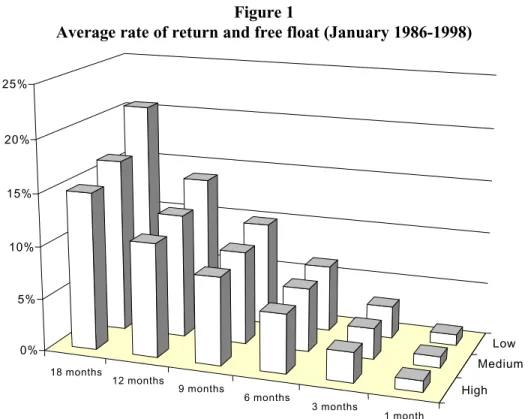
Figure 1 and Table 1 document the size effect in France over a twelve year period. 6 On the

first trading day of each month, three portfolios containing an equal number of stocks are formed based on their free float: low, medium, and high. The three portfolios’ returns including dividends are then measured over six holding periods - one, three, six, nine, twelve, and eighteen months.

Naturally, during a period when the French market's total rate of return has been over 130%, the longer the holding period, the higher the return for all three portfolios. But whatever the holding period, the low free float portfolio has a higher return than the high free float portfolio – significantly so for any period greater than or equal to three months.

Figure 1

Average rate of return and free float (January 1986-1998)

1 month 3 months 6 months 9 months 12 months 18 months High Medium Low 0% 5% 10% 15% 20% 25%

Note : Each stock out of a universe of approximately 150 stocks is assigned to one of three portfolios based upon its free float. Rates of return are measured after the formation of the portfolios.

6

Table 1

Size Effect (January 1986 – January 1998)

Free Float All Number of T-Test

High Medium Low stocks observations (Low-High)

Average rate of return

1 month 1.11% 1.10% 1.42% 1.21% 20,299 1.08 3 months 3.04% 3.14% 3.96% 3.38% 19,804 1.91 6 months 5.68% 6.04% 7.04% 6.25% 19,068 2.56 9 months 8.34% 8.75% 10.34% 9.13% 18,340 3.30 12 months 10.85% 11.62% 14.01% 12.13% 17,619 4.47 18 months 14.84% 16.44% 21.17% 17.39% 16,266 6.64

Standard deviation of rates of return

1 month 8.78% 9.33% 22.14% 14.80% 3 months 14.91% 16.20% 36.23% 24.48% 6 months 21.49% 23.38% 36.58% 27.93% 9 months 27.03% 29.51% 39.04% 32.22% 12 months 31.82% 35.57% 43.51% 37.21% 18 months 39.80% 44.37% 57.20% 47.52%

Note : This table lists the portfolios’ rates of return and their standard deviation after their formation, as well as the number of observations for a universe of approximately 150 stocks and the Student t-value of differential returns between opposite free float classes.

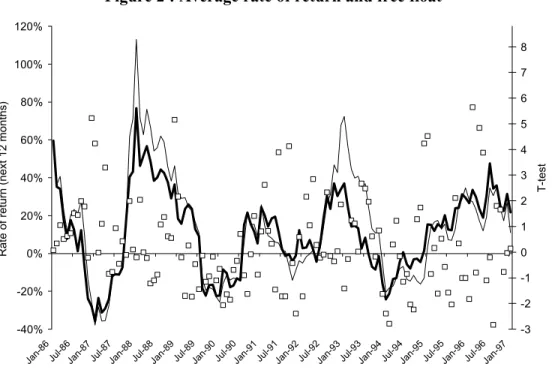
These results are all average results over many periods – from 144 one-month holding periods to 128 eighteen-month holding periods – which mask wide differences in period by period results. Figure 2 shows month by month rates of return over the 1986-1998 period for holding periods of twelve consecutive months. As documented on other markets, the size effect exists on average but can also appear in the opposite direction for long periods of time. This is the case for portfolios formed in 1992 and from July 1994 to July 1995, for example.

One should note the strong discrepancy in the standard deviation of rates of return for high and medium free float portfolios on the one hand and low free float portfolios on the other (Table 1). This is true for any holding period but is especially the case for the shorter holding periods. Liquidity, as measured by free float, might thus be another proxy for risk. These results confirm Knetz and Ready’s (1997), who show in a study on NYSE, Amex, and NASDAQ stocks that the size effect disappears if 16 out of 396 months for the 1963-1990 period are deleted or if 1% of the stocks are cut through a trimmed regression.

Figure 2 : Average rate of return and free float -40% -20% 0% 20% 40% 60% 80% 100% 120%

Jan-86 Jul-86Jan-87 Jul-87Jan-88 Jul-88Jan-89 Jul-89Jan-90 Jul-90Jan-91 Jul-91Jan-92 Jul-92Jan-93 Jul-93Jan-94 Jul-94Jan-95 Jul-95Jan-96 Jul-96Jan-97

Rate of return (next 12 months)

-3 -2 -1 0 1 2 3 4 5 6 7 8 T-test

Note : The bold line shows the one year rate of return of a portfolio containing the third of stocks with the highest free float. The thin line shows the one year rate of return of a portfolio containing the third of stocks with the lowest free float. Portfolios are formed monthly on the dates indicated on the x-axis. The squares give the Student t-values of differential returns between the two portfolios for each month (right-hand scale).This phenomenon isn’t limited to the month of January, as illustrated in Table 2. The table reports monthly returns over the entire 1986 – 1998 period for portfolios containing an equal number of stocks ranked by liquidity as measured by their free float. Significant differential positive returns between the low and high liquidity portfolios appear not only in January but also in February, April, and December. Negative differential returns appear in six other months, but are not significant.

Table 2: Liquidity and monthly returns

Free Float All T-test Average

High 2 Low Stocks L-H Liq premium

January 3.83% 4.54% 6.09% 4.82% 3.31 -0.44 February 1.23% 1.79% 2.07% 1.70% 1.65 -0.35 March 4.13% 3.26% 4.07% 3.82% -0.12 -0.32 April -0.88% -0.21% 0.50% -0.19% 2.96 -0.36 May -0.24% 0.10% -1.68% -0.61% -2.53 -0.33 June 2.24% 1.42% 0.50% 1.38% -3.23 -0.37 July -1.37% -0.77% -0.56% -0.90% 1.34 -0.39 August 1.67% 0.95% 3.52% 2.05% 0.65 -0.42 September -1.42% -2.06% -2.96% -2.15% -2.59 -0.44 October -0.73% -0.47% -1.59% -0.93% -1.53 -0.52 November 2.25% 1.64% 1.18% 1.69% -1.83 -0.59 December 2.59% 3.06% 5.88% 3.85% 4.85 -0.58 All months 1.11% 1.10% 1.42% 1.21% 1.08

Note : The differential returns between high and low free float portfolios yield a significant Student t-test (L-H) in only four months (bold figures). In December, for example, the liquidity premium is computed as at end of December and the returns are from end of December to end of January. Liquidity premiums of December and January pooled together are not statistically significant compared with a pool of all other months (t=1.17).

The rest of this paper is an attempt to take advantage of the “ex post” size effect phenomenon on an “ex ante” basis. We investigate both the ex ante risk and liquidity premiums. In the next section, we define the methodology and measurement of the two premiums.

2 . R

L

P

2.1. Methodology and data

The data used to measure the risk premium and liquidity premium are expectational data from Associés en Finance as published each month in their Security Market Line service. The Security Market Line provides endogenous CAPM expected risk and return figures for approximately 150 stocks representing about 90% of the total French market capitalization. CAPM-exogenous liquidity premiums are then derived as explained below.

Associés en Finance estimates the required rate of return by equalizing the stock price and the series of discounted future dividends forecast by financial analysts. These series are estimated from earnings per share and dividend forecasts for the next five years, and from a model beyond the fifth year. The estimated risk is obtained on a monthly basis from a combination of four risk factors: the duration of the stock (calculated from the sequence of the stock's future dividends relative to those of the market as a whole), the forecast risk, the financial risk, and the historical beta of the market sector to which the company belongs.

This representation results in a cloud of points in a two-dimensional plane of estimated risk (x-axis) and expected return (y-(x-axis), whose regression gives rise to the Security Market Line. Once the risk of a particular stock is established, the equilibrium rate of return in the CAPM sense is obtained for a given stock and a given month by a direct read; the Security Market Line gives the equilibrium rate of return.

The risk premium is defined as the difference between the expected return for the 150 stocks and the risk free rate (approximated by the French Treasury 10 year bond yield). The CAPM allows a split of the observed return in a given month in two parts: the first represents the normal return or the risk-adjusted equilibrium return, the other part is an excess return which reflects a misevaluation. The distance for a given stock between the computed required rate of return and the equilibrium rate of return is interpreted as a misevaluation.

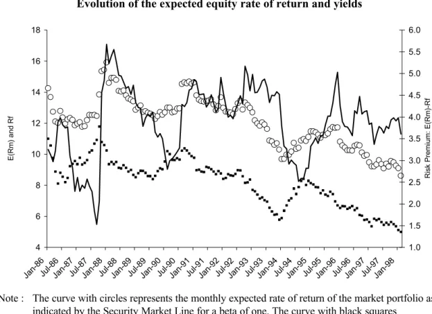
Figure 3 represents the evolution of the risk free rate as estimated by the return of the French 10 year OAT (Obligations Assimilables du Trésor, the equivalent of US Treasury bonds), and the expected rate of return of the market (in the CAPM sense).

Figure 3

Evolution of the expected equity rate of return and yields

4 6 8 10 12 14 16 18 Jan-86Jul-86Jan-87Jul-87Jan-88Jul-88Jan-89Jul-89Jan-90Jul-90Jan-91Jul-91Jan-92Jul-92Jan-93Jul-93Jan-94Jul-94Jan-95Jul-95Jan-96Jul-96Jan-97Jul-97Jan-98 E(Rm) and Rf 1.0 1.5 2.0 2.5 3.0 3.5 4.0 4.5 5.0 5.5 6.0

Risk Premium: E(Rm)-Rf

Note : The curve with circles represents the monthly expected rate of return of the market portfolio as indicated by the Security Market Line for a beta of one. The curve with black squares

represents the evolution of 10 years Treasury bond yields (a proxy for the risk-free rate). The rates from both curves can be read directly using the left-hand-side y-axis. The plain curve shows the evolution of the difference between the two other curves, defined as the risk premium, (read directly with the right-hand-side y-axis).

Although the CAPM doesn't deal with liquidity and the liquidity premium as an explanatory factor of expected return, its empirical version as implemented by Associés en Finance computes a liquidity premium as the OLS regression coefficient of the expected rate of return of each stock on the log of its free float. The liquidity premium for a given month is the slope of this regression line.

Table 3 gives sample statistics for the risk and liquidity premiums over the entire 1986-1998 period as well as over two subperiods: 1986 - June 1991 and July 1991 - January 1998. The risk premium is very close in both subperiods, with less variance during the second subperiod. The average liquidity premium is negative in both subperiods, -0.39 and -0.49 respectively, with large variations. This means that on average, investors require between 40 and 50 basis points more return annually on stocks with a lower liquidity as measured by their free float.

Table 3

Risk and liquidity premiums

Jan 86 to June 91 July 91 to Jan 98 Jan 86 to Jan 98 Liquidity premium Risk premium Liquidity premium Risk premium Liquidity premium Risk premium Average -0.39 3.79 -0.49 3.97 -0.44 3.89 Standard deviation 0.51 0.99 0.26 0.61 0.39 0.81 Maximum 0.54 5.67 0.18 5.17 0.54 5.67 Minimum -1.64 1.53 -1.12 2.52 -1.64 1.53

We then use a multivariate approach, and regress the expected return with the liquidity and the risk measures simultaneously in order to check whether liquidity is not another proxy for risk. Using the hypothesis of linearity in a multivariate approach, a joint estimate of the liquidity premium and the risk premium is made with an OLS regression from the following model:

2 i 1 i 0 i a Risk a Liquidity a ERR = + × + × (1)

Figure 4: Risk Premium 1 1.5 2 2.5 3 3.5 4 4.5 5 5.5

Jan-86May-86Sep-86Jan-87May-87Sep-87Jan-88May-88Sep-88Jan-89May-89Sep-89Jan-90May-90Sep-90Jan-91May-91Sep-91Jan-92May-92Sep-92Jan-93May-93Sep-93Jan-94May-94Sep-94Jan-95May-95Sep-95Jan-96May-96Sep-96Jan-97May-97Sep-97Jan-98

Note : The volatile line represents the evolution of the risk premium month after month (horizontal axis). The historical values of the risk premium at each date plus or minus one-third of the standard deviation constitute a tunnel whose boundaries are the two smooth lines.

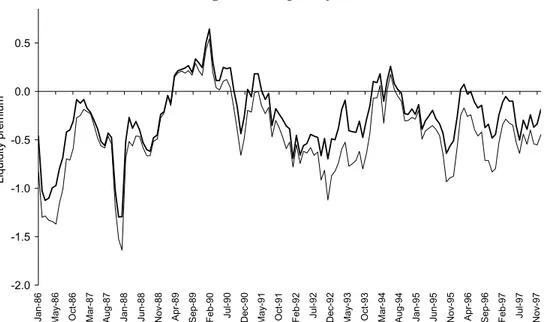
Figure 5: Liquidity Premium

-2.0 -1.5 -1.0 -0.5 0.0 0.5

Jan-86 _May-86 Oct-86 Mar-87 Aug-87 Jan-88 Jun-88 Nov-88 Apr-89 Sep-89 Feb-90 Jul-90 Dec-90 May-91 Oct-91 Feb-92 Jul-92 Dec-92 May-93 Oct-93 Mar-94 Aug-94 Jan-95 Jun-95 Nov-95 Apr-96 Sep-96 Feb-97 Jul-97 Nov-97

Liquidity premium

Note : The correlation between the two series is equal to 96%. The bold line shows the univariate estimate; the thin line shows the bivariate estimate according to equation (1).

The risk premium is a1 . The liquidity premium is a2 . Figure 4 and Figure 5 show the

and multivariate estimates of the risk and liquidity premium is in fact very high, so the following results will be reported using the univariate estimates.

2.2. Expected risk, liquidity, and expected return

The equilibrium rate of return is negatively linked to the free float (Table 4). Estimated risk is not the only variable explaining the differences in expected returns.

The comparison of the results obtained when the expected rate of return is used instead of the equilibrium rate of return yields some interesting results: in each risk class the difference in rates of return among free float classes is more pronounced when the expected rate of return is considered (Panel B). This would suggest that part of the difference between each stock and the Security Market Line is a compensation for differences in liquidity.

Table 4

Expected return, risk, and free float Panel A : expected equilibrium rate of return

High Free float Medium Free float Low Free float All stocks Student (Low-High) Low risk 11.53 11.39 11.66 11.53 2.31 Medium risk 12.02 12.02 12.25 12.10 4.87 High risk 12.58 12.59 12.85 12.68 5.66 All stocks 12.04 12.02 12.27 12.11 7.84 Student (High-Low) 21.17 24.45 23.78 40.06

Panel B : expected rate of return

High Free float Medium Free float Low Free float All stocks Student (Low-High) Low risk 11.41 11.53 11.63 11.52 3.44 Medium risk 11.74 11.93 12.45 12.04 10.90 High risk 12.56 12.52 13.10 12.73 7.76 All stocks 11.90 12.01 12.42 12.11 13.11 Student (High-Low) 18.64 13.83 20.45 30.50

Note : Expected equilibrium rate of return (Panel A) is the expected return on the Security Market Line (SML) for a given level of expected risk. Expected rate of return (Panel B) is the discount rate which equalizes anticipated dividends and the current stock price.

3. L

,

This section tests whether the liquidity premium and the risk premium are of any use in terms of market timing and tactical asset allocation. When the premiums give clear signals in a given month, we perform simulations using the entire universe of stocks for holding periods from one to eighteen months long. Similarly, we perform asset allocation simulations based on individual stocks’ liquidity and risk characteristics. We first present overall results, then specific month-by-month results.

3.1. Liquidity premium

Whenever the liquidity premium is unusually high or low, portfolios are formed according to the liquidity of individual stocks, and the subsequent returns are computed. In order to test whether the liquidity premium could be used as a tactical asset allocation indicator, we formed three sets of months based on the value of the liquidity premium from January 1989 to January 1998. The three previous years (1986-1988) are used to compute an historical mean and a standard deviation in order to determine January 1989’s liquidity class and eliminate any forward-looking bias. With the passage of time from 1989 on, each month's liquidity premium is added to the past historical series to update the mean and the standard deviation. The historical mean of the liquidity premium plus or minus one-third of the standard deviation determines the class thresholds each month from January 1989 to January 1998, thereby constituting a tunnel. The liquidity premium is considered high if it’s above the tunnel’s absolute value upper limit; it’s considered low if it is below the lower limit. We chose one-third of the standard deviation to determine the class thresholds because this results in a fairly uniform distribution of months above, below and within the tunnel.

Table 5

Liquidity premium, free float, and subsequent returns Panel A : 30 high liquidity premium months High Free Float Medium Free Float Low Free Float All stocks Number observations T-test (Low-High) 1 month 2.24% 2.60% 3.53% 2.79% 4,574 3.41 3 months 6.06% 7.40% 9.66% 7.69% 4,504 5.68 6 months 10.90% 13.84% 17.51% 14.03% 4,411 7.36 9 months 14.58% 18.05% 21.31% 17.91% 4,197 5.92 12 months 18.67% 23.43% 27.62% 23.11% 4,116 6.21 18 months 22.76% 34.64% 44.19% 33.30% 3,436 9.81

Panel B : 38 medium liquidity premium months

1 month 0.92% 0.77% 0.40% 0.69% 5,654 -1.84 3 months 2.94% 2.62% 1.29% 2.28% 5,318 -3.44 6 months 6.79% 6.76% 4.33% 5.97% 4,822 -3.31 9 months 10.29% 11.11% 10.00% 10.47% 4,452 -0.27 12 months 13.34% 14.09% 13.11% 13.51% 4,109 -0.17 18 months 22.14% 22.91% 22.21% 22.42% 3,723 0.04

Panel C : 42 low liquidity premium months

1 month 0.94% 0.69% 0.99% 0.87% 7,271 0.20 3 months 2.17% 1.70% 2.15% 2.00% 7,202 -0.04 6 months 3.85% 2.93% 3.58% 3.46% 7,094 -0.37 9 months 6.38% 4.53% 6.06% 5.66% 6,995 -0.35 12 months 8.07% 6.61% 9.14% 7.94% 6,745 0.97 18 months 10.05% 7.78% 10.91% 9.58% 6,540 0.61

Panel D : All 110 months

1 month 1.27% 1.22% 1.46% 1.32% 17,499 1.07 3 months 3.44% 3.49% 3.85% 3.60% 17,024 1.35 6 months 6.64% 7.02% 7.52% 7.05% 16,327 1.92 9 months 9.71% 10.04% 11.22% 10.31% 15,644 2.52 12 months 12.47% 13.32% 15.20% 13.64% 14,970 3.68 18 months 16.57% 18.71% 21.99% 19.02% 13,699 5.34

Panel E : T-Test (Panel A - Panel C)

1 month 4.66 6.28 6.97 10.43 3 months 8.35 10.93 11.88 18.08 6 months 10.46 14.31 15.06 23.07 9 months 9.56 14.04 12.96 21.10 12 months 10.34 13.91 12.36 21.01 18 months 9.14 16.67 15.13 23.49

Note : Portfolios are formed from January 1989 to December 1997, according to the value of the expected liquidity premium (in absolute value). Ex-post returns are computed from February 1989 to January 1998. Panel E tests the significance of the difference between the returns of panel A and C for the six different holding periods.

A total of 110 months are available. The first set of months includes 30 months where the liquidity premium has a high absolute value (the average historical value known at a given month, minus one third of the standard deviation), the second set includes 38 months with a medium liquidity premium (within the historical average plus or minus one third of the standard deviation). The third set includes 42 months with a low liquidity premium. The complete results are presented in Table 5 for the three sets of months under Panels A, B, and C and for all 110 months under Panel D. A t-test of differential returns between months with extreme liquidity premiums is presented in Panel E.

Some of the results in Table 5 appear graphically in Figure 6. Table 5 indicates that a portfolio containing low free float stocks in a given month has a higher rate of return in the subsequent year if the liquidity premium is high (in absolute value) in the month of formation (Panel A). For example, over a 12-month holding period following the observation in a given month of a high liquidity premium, low free float portfolios exhibit an average return of 27.62% compared with an average return of 18.67% for high free float portfolios. The ranking of the three portfolios' returns is the same and remains statistically significant over any holding period from one to 18 months. When the liquidity premium is high, the market prices the liquidity, and the holding of illiquid stocks (low free float) is rewarded. The reverse isn't observed when the liquidity premium is low: the returns of a high free float portfolio aren't significantly different statistically from the returns of low free float portfolios. Moreover, differential returns in Panels B and C between extreme portfolios in terms of liquidity are rarely statistically significant.

Interestingly enough, this last observation leads to another conclusion. When the liquidity premium is high, not only do low free float portfolios significantly outperform high free float portfolios, but all portfolios exhibit a strong performance. On the other hand, when the

liquidity premium is low, all portfolios exhibit a mediocre performance, far below the average performance of all stocks for all months ("All stocks" column in Panel D).

Figure 6

Liquidity premium, free float and subsequent average rate of return Panel A : High liquidity premium Panel C : Low liquidity premium

1 h 3 6 h 9 h 12 h 18 h Total average

High Free Float 2

Low Free Float 0% 5% 10% 15% 20% 25% 30% 35% 40% 45% 1 month 3 months 6 months 9 months 12 months 18 months

High Free Float 2

Low Free Float Total average 0% 2% 4% 6% 8% 10% 12% 14% 16% 18% 20%

Note : The thresholds which define whether the liquidity premium is high or low are recomputed each month using the entire historical series. For each month with a high (in absolute value) liquidity premium (in panel A) or a low liquidity premium (in panel C), three portfolios are formed following the stock’s free float. The three portfolios’ rates of return are computed for a period of eighteen months after the formation date. "Total average" is the evolution of the average observed return for all months and all stocks.

The liquidity premium seems to be a leading indicator of future overall market performance under certain circumstances and a prime factor for tactical asset allocation between liquidity classes. However, its practical implementation can be problematic, as the distribution of the largest 150 stocks in terms of market capitalization is skewed towards large market caps. The third of stocks with the highest free float accounted for 65% of the total market capitalization at the beginning of the period, and for more than 80% at the end of 1997 (Figure 7). In the meantime, liquidity class 2 shrank from over 20% of the total to less than 15%; liquidity class 3 went from 12.5% to 5%.

Figure 7

Liquidity class weights in terms of market capitalization

60% 65% 70% 75% 80% 85% 90% 95% 100% Feb-86Jun-86Oct-86Feb-87Jun-87Oct-87Feb-88Jun-88Oct-88Feb-89Jun-89Oct-89Feb-90Jun-90Oct-90Feb-91Jun-91Oct-91Feb-92Jun-92Oct-92Feb-93Jun-93Oct-93Feb-94Jun-94Oct-94Feb-95Jun-95Oct-95Feb-96Jun-96Oct-96Feb-97Jun-97Oct-97

Note : Each month the stocks are spread equally across three free float classes. The figure shows the weight of each class as a percentage of the total market cap. The high free float class is at the bottom, the low free float class is on top.

3.2. Risk premium

As we did for the liquidity premium, we used January 1986 to January 1989 to compute an historical mean and a standard deviation in order to determine January 1989’s risk class and eliminate any forward-looking bias. Thresholds are again set at one-third of the standard deviation because this results in a uniform distribution of months above, below and within the tunnel. There is a total of 110 months over the test period (Table 6), including 44 with a high risk premium (Panel A, below the lower threshold), 28 with a low risk premium (Panel C, above the upper threshold), and 38 with a medium risk premium (Panel B). Panel D presents the performance results for all months and Panel E gives the t-tests of differential returns between Panel A and Panel C portfolios. Like the historical average liquidity premium, the

historical average risk premium and its standard deviation are recomputed each month after January 1989.

When the risk premium is unusually high, high risk portfolios outperform low risk portfolios -significantly so beyond a one month holding period. When the risk premium is unusually low, low risk portfolios outperform high risk portfolios, again, significantly so beyond a one month holding period. The risk premium helps to identify attractive asset classes in terms of risk. Like the liquidity premium, it also seems to be a leading indicator of future overall market performance (Figure 8). Indeed, when the risk premium is low, future market performance is dismal, significantly below the average for the period (one example of average performance is 13.64% for a 12-month holding period for all months).

Figure 8

Risk premium and subsequent returns

Panel A : High risk premium Panel C : Low risk premium

1 month 3 months 6 months 9 months 12 months 18 months All stocks Low risk 2 High risk 0% 5% 10% 15% 20% 25% 30% 35% 1 month 3 months 6 months 9 months 12 months 18 months Low risk 2 High risk All stocks -10% -5% 0% 5% 10% 15% 20%

Table 6

Risk premium and subsequent returns Panel A : 44 high risk premium months

Low risk Medium

risk

High risk All stocks Number of

observations T-test (H-L) 1 month 2.52% 3.34% 2.86% 2.91% 8,064 1.33 3 months 7.27% 9.04% 8.20% 8.16% 7,951 2.18 6 months 13.62% 16.55% 16.23% 15.47% 7,808 4.06 9 months 17.57% 21.18% 21.22% 20.00% 7,679 4.21 12 months 21.08% 26.05% 26.57% 24.57% 7,548 5.05 18 months 26.19% 31.68% 32.44% 30.09% 7,195 4.21

Panel B : 38 medium risk premium months

1 month 1.30% 1.27% 0.91% 1.15% 5,416 -1.39 3 months 2.52% 2.43% 0.88% 1.93% 5,095 -3.22 6 months 6.32% 5.34% 3.70% 5.11% 4,593 -3.40 9 months 9.03% 7.37% 5.12% 7.17% 4,118 -3.81 12 months 9.81% 7.15% 4.43% 7.13% 3,911 -4.31 18 months 14.16% 11.03% 6.98% 10.70% 3,113 -4.11

Panel C : 28 low risk premium months

1 month -1.28% -1.88% -1.80% -1.65% 4,019 -1.57 3 months -2.65% -3.63% -3.87% -3.39% 3,978 -2.21 6 months -5.83% -7.20% -9.06% -7.40% 3,926 -4.44 9 months -3.07% -5.03% -8.60% -5.64% 3,847 -6.13 12 months 1.05% -1.41% -7.09% -2.61% 3,511 -7.11 18 months 9.72% 5.39% -4.90% 3.15% 3,391 -9.47

Panel D : all 110 months

1 month 1.27% 1.50% 1.19% 1.32% 17,499 -0.46 3 months 3.53% 4.09% 3.20% 3.60% 17,024 -1.14 6 months 6.91% 7.69% 6.61% 7.05% 16,327 -0.66 9 months 10.27% 11.11% 9.62% 10.31% 15,644 -1.11 12 months 13.49% 14.68% 12.81% 13.64% 14,970 -0.93 18 months 19.44% 20.57% 17.15% 19.02% 13,699 -2.32

Panel E : T-tests (Panel A – Panel C)

1 month 13.99 17.24 14.56 26.29 3 months 21.88 25.90 22.70 40.44 6 months 31.50 35.70 33.73 57.87 9 months 25.76 30.70 31.09 50.42 12 months 19.16 25.11 28.45 42.15 18 months 11.28 17.40 23.83 30.65

Note : Portfolios are formed from January 1989 to December 1997, following the value of the expected risk premium. Ex-post returns are computed from February 1989 to January 1998. Panel E tests the significance of the difference between the returns of panel A and C for the 6 different holding periods.

The practical implementation of the risk premium’s indications in terms of future overall market performance and tactical asset allocation seems much easier than practical implementation of the liquidity premium’s indications. Each risk class in our universe of 150 French stocks has about the same market capitalization (Figure 9).

Figure 9

Risk class weights in terms of market capitalization

0% 10% 20% 30% 40% 50% 60% 70% 80% 90% 100% Jan-86Jul-86Jan-87Jul-87Jan-88Jul-88Jan-89Jul-89Jan-90Jul-90Jan-91Jul-91Jan-92Jul-92Jan-93Jul-93Jan-94Jul-94Jan-95Jul-95Jan-96Jul-96Jan-97Jul-97Jan-98 Note : Each month the stocks are spread equally across three risk classes. The figure shows the weight

of each class as a percentage of the total market capitalization. The low risk class is at the bottom, the high risk class is on top.

3.3. Risk and liquidity premiums in tandem

The two previous subsections present important results in terms of market timing and asset allocation.

In terms of market timing, both the liquidity premium and –even more so– the risk premium are indicators of future overall market performance. When they are high, i.e. when the market

above average for periods of one month up to eighteen months. Conversely, when the market doesn’t price risk and illiquidity correctly, future overall market performance is poor.

In terms of asset allocation, both the risk and the liquidity premiums are discriminant factors. In months where the risk premium is high, the portfolio containing high risk securities vastly outperforms the portfolio of low risk securities, and vice versa. In months where the liquidity premium is high, low free float securities significantly outperform high free float securities. In this section, we combine the information in the risk premium and the information in the liquidity premium to form portfolios and ask ourselves whether the combined use of both premiums adds value in terms of market timing and asset allocation, beyond the information embedded in one or the other.

3.3.1. Liquidity and risk premiums and market timing

In this test, we select months according to the combined levels of both the risk and the liquidity premiums. Portfolio performance is measured over subsequent periods of up to eighteen months. Results are presented in Table 7, with some data from Tables 4 and 5.

Table 7

Market timing using risk and liquidity premiums: average subsequent returns and Student t-tests

Low Liquidity Premium Medium Liquidity Premium High Liquidity Premium

All months Number of

observations

T-test (High-Low)

Panel A : 44 high risk premium months

1 month 3.19% 0.99% 3.81% 2.91% 8,064 2.51 3 months 8.16% 5.11% 9.98% 8.16% 7,951 4.52 6 months 16.46% 9.93% 17.99% 15.47% 7,808 2.48 9 months 22.94% 16.18% 19.93% 20.00% 7,679 -3.70 12 months 28.29% 16.38% 26.51% 24.57% 7,548 -1.75 18 months 30.56% 23.62% 33.80% 30.09% 7,195 2.27

Panel B : 38 medium risk premium months

1 month 1.55% 1.49% -0.15% 1.15% 5,416 -5.33

6 months 4.01% 8.64% 2.67% 5.11% 4,593 -1.64

9 months 3.95% 9.32% 11.30% 7.17% 4,118 6.84

12 months 1.52% 13.66% 12.06% 7.13% 3,911 8.86

18 months -1.50% 29.29% 30.60% 10.70% 3,113 16.20

Panel C : 28 low risk premium months

1 month -2.12% -0.86% n.a. -1.65% 4,019 4.67 3 months -4.77% -1.04% n.a. -3.39% 3,978 8.38 6 months -10.59% -1.96% n.a. -7.40% 3,926 14.38 9 months -11.04% 3.64% n.a. -5.64% 3,847 19.10 12 months -9.13% 9.08% n.a. -2.61% 3,511 17.76 18 months -4.47% 16.79% n.a. 3.15% 3,391 15.22

Panel D : all 110 months

1 month 0.87% 0.69% 2.79% 1.32% 17,499 10.43 3 months 2.00% 2.28% 7.69% 3.60% 17,024 18.08 6 months 3.46% 5.97% 14.03% 7.05% 16,327 23.07 9 months 5.66% 10.47% 17.91% 10.31% 15,644 21.10 12 months 7.94% 13.51% 23.11% 13.64% 14,970 21.01 18 months 9.58% 22.42% 33.30% 19.02% 13,699 23.49

Panel E : T-tests (Panel A – Panel C)

1 month 21.05 6.67 12.46 26.29 3 months 30.99 13.08 15.23 40.44 6 months 45.47 17.98 19.29 57.87 9 months 45.32 13.31 8.25 50.42 12 months 41.54 5.99 12.33 42.15 18 months 27.28 4.29 1.57 30.65

Note : The T-tests in the last column of the table test the difference in the rate of return between high liquidity premium months and low liquidity premium months. Panel C contains no observations in the "high liquidity premium" class, so the T-tests in this case are between the medium class and the low liquidity premium class.

The 12-month subsequent performance of a portfolio containing all the stocks in our universe when both the risk and the liquidity premiums are low is -9.13%, for example, compared to -2.61% when months of portfolio formation are selected on the basis of a low risk premium only, or 7.94% on the basis of a low liquidity premium only, or an all-month, all-stock 12-month performance of 13.64%.

When both the risk and the liquidity premiums are unusually high, the corresponding returns are 26.51% (high risk and high liquidity premiums), compared to 24.57% when months of portfolio formation are selected on the basis of a high risk premium only (Panel A), or 23.11%

on the basis of a high liquidity premium (Panel D), or again, compared to the month, all-stock 12-month performance of 13.64%.

These kinds of results appear however long the portfolio is held. Thus the liquidity premium in tandem with risk premium provides additional information on subsequent overall market performance, marginally but still in a statistically significant way.

We reproduced month-by-month results in the Appendix for the 1986-1998 period to gain a better understanding of this phenomenon. The Appendix lists monthly risk and liquidity premiums and 12-month rates of return for the different risk and liquidity classes. One can determine at a glance in which months both the liquidity premium (LPC) and the risk premiums (RPC) were high (3 and 3) or low (1 and 1) and which were the subsequent 12-month returns on the same line for the different asset classes. For example, both premiums are low from October 1986 to October 1987, and so are the subsequent 12-month returns (the October 1987 crash helps, but remember from Table 3 that both premiums are very stable over the entire period). The same is true from January 1990 to July 1990. Conversely, both premiums are high from July 1992 to March 1993 with substantial 12-month subsequent returns, and a significant outperformance from risky and less liquid stocks. Such portfolios include between 9 and 18 stocks depending on the measurement period. Even if the amount of transaction costs could be overestimated, as shown by Constantinides (1986), and empirically determined on the French market by Handa et al. (1995), such strategies are low transaction cost strategies insofar as the risk and liquidity characteristics of individual stocks are fairly steady over time.

3.3.2. Liquidity and risk premiums and asset allocation

The previous section demonstrates how the combined use of the risk premium and the liquidity premium adds value compared to independent use of one or the other. The premiums signal whether to invest or not in our universe of stocks, irrespective of individual levels of risk or

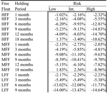
liquidity. In this section we use the levels of the risk premium and the liquidity premium in terms of both market timing and asset allocation. When both the risk premium and the liquidity premium are high, for example, it’s a signal to invest in equities, as demonstrated in the previous section. It’s also a signal to invest preferably in high risk and low free float stocks (strategy A). If the risk premium and the liquidity premium have any value in terms of asset allocation, such a strategy should lead to higher subsequent returns than other strategies: strategy A1, a portfolio of low risk and low free float stocks, strategy A2, a portfolio of high risk and high free float stocks, or even better, strategy A3, a portfolio of low risk and high free float stocks.

Table 8 shows the results of such strategies, with the subsequent returns of portfolios from one to 18 months after their formation. Let’s consider 12-month portfolio returns. Strategy A in Panel B leads to average subsequent 12-month returns of 37.67%, with corresponding returns of 28.70% for strategy A1, 19.31% for strategy A2, and 17.52% for strategy A3. These differential returns are statistically significant as they are over all holding periods beyond three months.

Table 8

Risk and liquidity premiums and asset allocation Panel A : Low Risk Premium and Low Liquidity Premium

Free Holding Risk

Float Period Low Int. High

HFF 1 month -1.02% -2.16% -2.32% HFF 3 months -2.16% -4.08% -5.55% HFF 6 months -6.20% -9.93% -12.81% HFF 9 months -5.23% -9.13% -14.83% HFF 12 months -4.09% -8.03% -14.70% HFF 18 months 1.37% -3.40% -10.62% MFF 1 month -2.15% -2.73% -2.03% MFF 3 months -4.19% -5.85% -4.81% MFF 6 months -9.08% -11.10% -9.63% MFF 9 months -8.39% -10.41% -9.70% MFF 12 months -5.15% -6.10% -7.82% MFF 18 months 1.83% 2.56% -8.96% LFF 1 month -2.17% -2.29% -2.23% LFF 3 months -5.49% -5.49% -5.38% LFF 6 months -13.02% -12.08% -11.73%

LFF 12 months -9.86% -12.18% -14.28% LFF 18 months 2.11% -8.04% -14.95%

Panel B : High Risk Premium and High Liquidity Premium

Free Holding Risk

Float Period Low Int. High

HFF 1 month 3.12% 3.57% 3.15% HFF 3 months 8.00% 8.93% 6.90% HFF 6 months 12.21% 14.84% 12.87% HFF 9 months 13.95% 16.35% 13.43% HFF 12 months 17.52% 22.96% 19.31% HFF 18 months 18.73% 24.85% 23.75% MFF 1 month 3.20% 4.49% 2.82% MFF 3 months 9.71% 11.67% 8.90% MFF 6 months 17.08% 19.23% 18.33% MFF 9 months 19.58% 20.32% 22.43% MFF 12 months 25.21% 26.06% 31.01% MFF 18 months 28.69% 34.36% 39.86% LFF 1 month 4.50% 4.91% 4.68% LFF 3 months 11.33% 12.61% 12.18% LFF 6 months 20.85% 23.00% 24.34% LFF 9 months 22.79% 24.46% 27.13% LFF 12 months 28.70% 32.06% 37.67% LFF 18 months 39.75% 42.70% 57.98%

Note : HFF stands for high free float, MFF for medium free float, and LFF for low free float. There are 3 risk premium classes, 3 liquidity premium classes, 3 risk classes, and 3 liquidity classes, for a total of 34=81 combinations. These tables show the 9 classes obtained when both premiums are low (Panel A) and the 9 classes obtained when both premiums are high (Panel B). In panel A the t-tests of the difference in rate of returns between north-west portfolio (low risk and high liquidity float, strategy B) and south east portfolio (high risk and low free float, strategy B3) are 1.58 for 1 month, 2.64 for 3 months, 3.61 for 6 months, 5.58 for 9 months, 5.28 for 12 months and 6.33 for 18 months. In panel B the t-tests of the difference in returns between north-west portfolio (low risk and high free float, strategy A3) and south east (high risk and low free float, strategy A) are –2.00 for 1 month, -3.25 for 3 months, -6.24 for 6 months, -5.21 for 9 months, -5.95 for 12 months and –7.33 for 18 months.

Conversely, when both the risk premium and the liquidity premium are low, this leads to concentration in low risk and high liquidity stocks (strategy B in Panel A). Strategy B should post better returns relative to strategy B1 (high risk and high free float stocks), strategy B2 (low risk and low free float stocks), or strategy B3 (high risk and low free float stocks). The returns of strategy B, B1, B2, and B3 for a 12-month holding period are -4.09%, -14.70%, -14.28%, and -9.86%, respectively. All results are in the right direction and statistically significant for all holding periods (except an 18-month holding period with strategy B2 which is not statistically significantly different from the other strategies).

4 . C

We have documented the existence of a size effect in France over the 1986-1998 period. This was done using free float rather than the relative spread or the market capitalization as a proxy for size and liquidity. Companies with a low free float tend to outperform large companies. As evidenced in the United States, this is true in January, but a significant size effect also appears in some other months.

Using a practical version of the CAPM with financial analysts’ expectations on future cash flows for a universe of about 150 French companies traded on the Paris Bourse and representing about 90% of the total French market capitalization, we defined a risk premium and a liquidity premium. While the risk premium is used in its well-known definition as the spread between the expected return of the equity market and the 10 year government bond yield 7, the liquidity premium is measured as the differential return between high and low free

float stocks.

We have shown that both the risk and the liquidity premium vary significantly over time with a mean-reverting tendency, as observed in many other economic series.

This mean-reverting phenomenon can be used effectively both for market timing and asset allocation. We have shown in this respect that the premiums can be used separately. Results are even more striking when the premiums are used in combination, which proves that additional information can be extracted from the liquidity premium on top of the risk premium. When both premiums are high, it is a strong signal that the future overall performance of the

7

We use a risk premium expressed in absolute value for the purpose of the present research. However a risk premium of 2% with interest rates at 4% probably doesn’t mean the same thing if interest rates are at 10%. If there are large variations in interest rate levels over the period, it might be necessary to use a risk premium expressed in a value relative to interest rates. Whether the risk premium is

equity market will be high. Moreover, in such cases, high risk and low liquidity stocks outperform the rest of the market. When both premiums are low, it is an indication of poor future performance. This is true over the entire period, and it is also true when one looks at month by month estimates of both premiums.

These results seem to validate our measurements of liquidity and the liquidity premium. Further work needs to be done, first to integrate liquidity in asset pricing models and second to identify the factors which can explain the level of the liquidity premium. This is the purpose of current research.

References

Amihud Y. and H. Mendelson, 1986, “Asset Pricing and the Bid-Ask Spread”, Journal of Financial Economics, Vol , n° 2, p. 223-249.

Banz R. W., 1981, “The Relationship Between Return and Market Value of Common Stocks”, Journal of Financial Economics, Vol. 9, n° 1, p. 3-18.

Brennan M. J. and A. Subrahmanyam, 1996, “Market Microstructure and Asset Pricing: On the Compensation for Illiquidity in Stock Returns”, Journal of Financial Economics, 41, July, p. 441-464.

Brown P., D.B. Keim, A.W. Kleidon and T.A. Marsh, 1983, “Stock Return Seasonalities and the Tax Loss Selling Hypothesis: Analysis of the Arguments and Australian Evidence”, Journal of Financial Economics, Vol 12, n° 1, p. 105-127.

Constantinides G., 1986, "Capital Market Equilibrium with Transaction Costs," Journal of Political Economy, 94, p. 842-862.

Engle R.F. and J. Lange, 1997, “Measuring, Forecasting and Explaining Time-Varying Liquidity in the Stock Market”, discussion paper, University of San Diego, California. Hamon J. and B. Jacquillat, 1992, Le marché français des actions. Etudes empiriques

1977-1991, Presses Universitaires de France.

Hamon J. and B. Jacquillat, 1997, “Expected Returns and Liquidity Premiums on the Paris Bourse: an empirical investigation”, CEREG Working paper, n° 9706, Université Paris-Dauphine.

Handa P., Hamon J., Jacquillat B. and R.A. Schwartz, 1995, “Market Structure and the Supply of Liquidity”, in Schwartz, R.A. (ed.), “Global Equity Markets”, Irwin.

expressed in absolute or relative terms doesn’t affect the rankings in this study: a month labeled “high risk premium” would receive the same label using a relative risk premium.

Jacoby G. and D. J. Fowler, 1997, “The capital asset pricing model and the liquidity effect: a theoretical approach”, Working paper, York University.

Jacquillat B., 1985, “Désétatiser”, Laffont.

Jousset H., 1992, "La liquidité," Analyse Financière, 4e trimestre, 91, p.78-87.

Keim D.B., 1983, “Size-related Anomalies and Stock returns Saisonality: further empirical evidence”, Journal of Financial Economics, Vol 12, n° 1, p. 13-32.

Knetz P.J. and M.J. Ready, 1997, « On the robustness of size and book-to-market in cross-sectional regressions », The Journal of Finance, Vol 52, n° 4, September, p. 1355-1382. Kyle A.S., 1985, "Continuous Auctions and Insider Trading," Econometrica, 53, p.

1315-1335.

Treynor J. L., 1978, "Liquidity, Interest Rates, and Inflation," unpublished manuscript.

Appendix

Month by month results

Rate of return (%) Rate of return (%) Premium

Date High Free Float Med. Free Float Low Free Float Low-High T Low Risk Med. Risk

High Risk

High-Low T Liquid ity LP C RP C Risk Jan-86 59.52 53.42 57.08 -2.44 -0.20 53.64 61.62 54.83 1.19 0.11 -0.81 3.25 Feb-86 35.29 47.08 36.25 0.96 0.11 29.63 51.45 37.66 8.03 0.97 -1.30 3 1 3.12 Mar-86 34.03 40.51 40.70 6.67 0.73 33.37 39.67 42.18 8.81 0.99 -1.29 3 1 2.97 Apr-86 17.24 27.98 22.19 4.95 0.63 12.16 27.62 27.61 15.45 1.97 -1.33 3 3 3.22 May-86 7.79 18.51 11.64 3.84 0.52 1.77 17.63 18.51 16.74 2.43 -1.34 3 3 3.89 Jun-86 17.66 26.02 20.22 2.56 0.34 6.78 32.18 25.25 18.48 2.86 -1.37 3 3 3.98 Jul-86 12.60 19.36 23.14 10.54 1.05 1.01 24.33 30.30 29.29 3.21 -1.16 1 3 3.82 Aug-86 1.21 15.17 21.20 19.99 1.99 -2.90 16.64 24.05 26.95 2.99 -1.02 1 3 3.75 Sep-86 12.25 18.23 27.55 15.30 1.52 1.12 26.72 30.78 29.66 3.29 -0.70 1 3 3.77 Oct-86 -7.29 0.12 9.74 17.03 1.85 -14.77 6.87 9.78 24.55 2.98 -0.71 1 1 3.10 Nov-86 -23.84 -21.44 -13.65 10.19 1.44 -27.00 -16.69 -16.02 10.98 1.69 -0.59 1 1 2.83 Dec-86 -28.00 -25.46 -25.67 2.33 0.34 -24.73 -29.12 -25.14 -0.41 -0.07 -0.27 1 1 2.29 Jan-87 -35.74 -35.44 -37.91 -2.17 -0.36 -33.14 -34.25 -41.52 -8.38 -1.95 -0.25 1 1 2.61 Feb-87 -23.50 -25.85 -28.26 -4.76 -1.01 -23.83 -24.82 -28.70 -4.86 -1.11 -0.19 1 1 2.29 Mar-87 -31.26 -31.63 -35.76 -4.50 -1.01 -28.82 -31.86 -37.60 -8.78 -2.22 -0.21 1 1 2.43 Apr-87 -29.05 -32.72 -35.59 -6.54 -1.42 -28.26 -32.28 -36.39 -8.12 -2.09 -0.23 1 1 2.36 May-87 -24.13 -26.63 -27.47 -3.34 -0.77 -22.00 -26.50 -29.52 -7.52 -1.86 -0.36 1 1 2.57 Jun-87 -11.58 -14.56 -12.87 -1.29 -0.27 -9.86 -15.78 -13.35 -3.50 -0.75 -0.48 1 1 2.41 Jul-87 -10.92 -16.23 -10.78 0.15 0.03 -11.02 -14.13 -12.98 -1.96 -0.42 -0.56 1 1 2.28 Aug-87 -11.12 -17.11 -10.79 0.33 0.07 -9.43 -15.04 -14.65 -5.21 -1.11 -0.58 1 1 1.84 Sep-87 -7.42 -13.29 -8.33 -0.91 -0.18 -8.16 -10.82 -10.01 -1.85 -0.36 -0.46 1 1 1.53 Oct-87 17.89 4.87 17.71 -0.18 -0.02 11.29 13.36 15.50 4.22 0.56 -0.55 1 1 2.06 Nov-87 40.36 32.70 61.70 21.34 2.16 34.72 51.55 47.86 13.14 1.24 -1.19 3 3 4.56 Dec-87 43.24 40.57 71.14 27.90 2.67 39.42 54.22 60.46 21.04 1.90 -1.52 3 3 4.84 Jan-88 76.74 73.27 112.97 36.23 2.48 63.88 94.56 103.10 39.21 2.61 -1.64 3 3 5.67 Feb-88 46.37 41.98 71.58 25.21 2.84 36.96 56.98 64.33 27.37 2.81 -0.69 2 3 5.23 Mar-88 51.56 47.38 62.72 11.15 1.24 36.06 56.99 67.30 31.24 3.22 -0.52 1 3 5.41 Apr-88 56.71 65.58 76.24 19.53 1.97 48.04 71.75 78.24 30.19 2.77 -0.56 1 3 5.55 May-88 48.45 59.87 66.57 18.12 1.80 42.86 59.75 72.15 29.29 2.97 -0.46 1 3 5.28 Jun-88 38.41 43.75 54.09 15.69 1.66 35.09 40.97 60.09 25.00 2.63 -0.47 1 3 4.96 Jul-88 40.13 45.42 55.91 15.77 1.78 40.17 46.72 54.77 14.60 1.66 -0.58 1 3 4.94 Aug-88 44.33 44.21 62.01 17.68 1.99 43.89 51.53 55.92 12.02 1.33 -0.67 2 3 4.81 Sep-88 42.48 49.25 58.83 16.35 2.04 49.10 46.93 54.65 5.55 0.57 -0.66 2 3 4.66 Oct-88 37.69 34.77 45.81 8.12 1.08 39.97 40.03 38.95 -1.02 -0.13 -0.51 1 3 4.70 Nov-88 29.02 28.40 38.16 9.14 1.37 34.05 34.47 27.92 -6.14 -0.95 -0.49 1 3 4.52 Dec-88 36.36 33.78 46.25 9.89 1.41 39.37 45.70 31.87 -7.50 -1.01 -0.28 1 3 4.73

Rate of return (%) Rate of return (%) Premium Date High Free Float Med. Free Float Low Free Float Low-High T Low Risk Med. Risk

High Risk

High-Low T Liquid ity LP C RP C Risk Feb-89 15.65 19.05 29.14 13.49 2.11 25.99 21.90 16.16 -9.84 -1.46 -0.05 1 3 4.22 Mar-89 23.48 20.16 29.48 6.01 0.84 30.57 24.67 17.80 -12.77 -1.87 -0.15 1 3 4.20 Apr-89 25.90 12.99 24.46 -1.44 -0.21 28.12 21.22 14.06 -14.05 -2.39 0.15 1 2 3.79 May-89 23.50 14.76 22.55 -0.95 -0.14 30.27 19.92 10.72 -19.55 -3.53 0.19 1 2 3.98 Jun-89 12.75 10.42 16.61 3.87 0.62 23.60 13.44 2.83 -20.77 -3.87 0.21 1 2 4.07 Jul-89 9.12 7.38 10.76 1.64 0.28 17.42 9.64 0.56 -16.86 -3.30 0.19 1 2 4.01 Aug-89 -18.50 -17.35 -13.03 5.48 1.11 -7.84 -19.06 -22.03 -14.18 -3.16 0.21 1 2 4.11 Sep-89 -22.38 -23.77 -19.39 2.99 0.59 -14.09 -24.56 -26.71 -12.62 -2.69 0.17 1 2 3.65 Oct-89 -16.76 -20.87 -17.95 -1.19 -0.22 -13.09 -16.08 -26.48 -13.39 -2.83 0.29 1 2 3.54 Nov-89 -16.65 -21.01 -18.95 -2.30 -0.45 -11.36 -18.68 -26.11 -14.75 -3.35 0.21 1 2 3.62 Dec-89 -22.47 -21.64 -22.92 -0.45 -0.10 -17.82 -20.80 -28.17 -10.34 -2.42 0.17 1 2 3.50 Jan-90 -22.21 -24.03 -25.74 -3.53 -0.88 -19.34 -21.55 -30.58 -11.23 -2.96 0.43 1 1 3.16 Feb-90 -8.51 -10.85 -16.08 -7.57 -1.83 -7.82 -9.48 -17.59 -9.78 -2.42 0.54 1 1 2.80 Mar-90 -10.46 -9.40 -11.31 -0.86 -0.23 -7.91 -8.45 -14.30 -6.40 -1.71 0.20 1 1 2.99 Apr-90 -17.79 -8.55 -14.06 3.73 0.93 -11.26 -12.09 -16.81 -5.55 -1.38 0.04 1 1 3.04 May-90 -16.98 -10.37 -12.91 4.07 1.04 -11.00 -13.07 -16.05 -5.04 -1.28 0.02 1 1 3.11 Jun-90 -13.08 -11.84 -13.48 -0.40 -0.10 -11.25 -13.21 -13.74 -2.49 -0.68 0.10 1 1 3.19 Jul-90 -14.13 -12.71 -13.51 0.62 0.15 -13.85 -11.10 -15.08 -1.23 -0.31 0.12 1 1 3.29 Aug-90 14.88 11.63 5.54 -9.34 -1.73 7.69 16.56 8.69 0.99 0.19 0.04 1 3 4.29 Sep-90 21.53 19.55 21.66 0.13 0.02 19.26 26.11 18.05 -1.21 -0.19 -0.17 1 3 4.24 Oct-90 15.59 13.39 15.55 -0.04 -0.01 14.09 14.63 15.72 1.63 0.28 -0.39 2 3 4.33 Nov-90 11.50 13.56 15.26 3.77 0.62 11.89 12.43 15.59 3.69 0.61 -0.66 3 3 4.62 Dec-90 5.29 2.82 8.79 3.50 0.56 3.57 4.38 8.47 4.90 0.81 -0.49 2 3 4.65 Jan-91 24.48 16.11 25.66 1.18 0.16 17.43 21.65 26.58 9.15 1.37 -0.20 1 3 4.86 Feb-91 20.18 5.55 14.63 -5.54 -0.87 8.45 15.05 16.93 8.48 1.42 -0.21 1 3 4.81 Mar-91 14.15 8.40 9.38 -4.77 -0.76 7.00 14.18 11.07 4.07 0.69 -0.01 1 3 4.51 Apr-91 18.48 7.63 7.89 -10.60 -1.72 6.32 15.16 13.04 6.73 1.07 0.00 1 3 4.52 May-91 19.43 15.15 5.99 -13.44 -2.40 7.47 17.75 15.56 8.10 1.41 -0.15 1 3 4.53 Jun-91 11.51 11.53 5.39 -6.12 -1.09 5.83 14.07 9.04 3.21 0.58 -0.23 2 3 4.23 Jul-91 2.40 7.18 1.26 -1.14 -0.20 -0.59 9.37 2.43 3.02 0.55 -0.16 1 3 4.31 Aug-91 -1.27 6.51 1.21 2.48 0.43 -1.33 8.02 -0.09 1.25 0.22 -0.47 2 3 4.51 Sep-91 -0.52 -4.03 -6.90 -6.38 -1.22 -1.44 -3.34 -6.20 -4.75 -0.90 -0.30 2 3 4.32 Oct-91 -4.12 -4.43 -14.15 -10.03 -2.03 -5.44 -5.14 -11.68 -6.24 -1.21 -0.37 2 2 4.11 Nov-91 -1.15 1.80 -8.87 -7.72 -1.62 0.70 -1.52 -7.05 -7.75 -1.47 -0.47 2 3 4.20 Dec-91 12.25 15.30 -3.82 -16.06 -2.82 8.08 10.35 5.68 -2.40 -0.41 -0.59 3 3 4.91 Jan-92 2.71 2.70 -5.06 -7.77 -1.61 4.83 -0.20 -4.16 -8.99 -1.66 -0.53 2 3 4.57 Feb-92 3.13 4.99 -1.73 -4.86 -1.10 7.97 -0.51 -1.17 -9.14 -1.82 -0.78 3 3 4.26 Mar-92 7.12 6.89 -0.37 -7.49 -1.58 13.12 4.79 -4.38 -17.49 -3.50 -0.55 2 2 4.00 Apr-92 2.05 8.16 1.69 -0.36 -0.08 11.77 1.06 -1.10 -12.87 -2.45 -0.75 3 2 4.04 May-92 -4.39 1.46 -1.95 2.43 0.53 7.48 -3.80 -8.82 -16.30 -3.22 -0.62 3 2 3.96 Jun-92 4.90 11.32 2.74 -2.16 -0.43 13.03 7.48 -1.62 -14.65 -2.62 -0.64 3 2 4.16 Jul-92 18.74 21.09 14.10 -4.63 -0.84 23.80 19.14 11.21 -12.59 -2.11 -0.58 3 3 4.30 Aug-92 30.36 36.08 26.81 -3.55 -0.57 33.47 28.42 31.18 -2.29 -0.35 -0.66 3 3 4.49 Sep-92 23.46 37.63 31.11 7.65 1.23 33.02 28.16 30.06 -2.96 -0.46 -0.63 3 3 4.30 Oct-92 37.04 52.09 46.82 9.78 1.28 43.94 41.58 49.46 5.52 0.69 -0.92 3 3 5.17 Nov-92 30.41 47.79 42.66 12.25 1.74 39.99 38.56 41.41 1.43 0.20 -0.81 3 3 4.97 Dec-92 33.99 59.04 67.49 33.50 4.13 54.00 52.80 50.67 -3.34 -0.41 -1.12 3 3 4.60 Jan-93 37.01 64.10 72.50 35.49 4.52 50.34 61.54 58.68 8.34 1.06 -0.87 3 3 4.98 Feb-93 24.23 46.06 56.09 31.86 5.16 39.63 42.38 41.05 1.42 0.21 -0.83 3 3 4.56 Mar-93 14.17 31.35 44.43 30.26 5.23 24.42 29.86 32.21 7.79 1.24 -0.74 3 3 4.57 Apr-93 14.49 28.81 39.80 25.31 4.24 16.87 31.06 32.19 15.32 2.51 -0.59 2 3 4.68 May-93 13.41 27.59 40.74 27.33 4.85 16.17 30.09 32.65 16.48 2.70 -0.52 2 3 4.83 Jun-93 2.65 18.81 35.36 32.71 5.64 9.36 18.73 26.29 16.93 2.58 -0.77 3 3 4.87 Jul-93 8.33 22.47 36.77 28.44 4.23 10.07 24.40 30.91 20.84 3.08 -0.75 3 3 4.68 Aug-93 -0.39 12.70 24.30 24.69 3.88 2.50 13.27 17.80 15.30 2.45 -0.71 3 3 4.33 Sep-93 -7.09 3.21 13.04 20.13 3.89 -5.43 5.60 6.95 12.38 2.36 -0.62 3 3 4.50 Oct-93 -8.54 -3.75 10.79 19.33 3.30 -9.86 0.86 5.05 14.91 2.63 -0.80 3 3 4.49 Nov-93 -1.30 -1.94 10.77 12.07 2.17 -6.25 1.18 10.78 17.03 3.43 -0.64 3 3 4.58 Dec-93 -16.06 -13.73 -5.56 10.50 2.62 -18.74 -11.64 -5.65 13.10 3.62 -0.43 2 3 4.52 Jan-94 -24.19 -24.51 -20.41 3.77 1.11 -27.67 -22.02 -19.57 8.10 2.49 -0.07 1 2 3.80

Rate of return (%) Rate of return (%) Premium Date High Free Float Med. Free Float Low Free Float Low-High T Low Risk Med. Risk

High Risk

High-Low T Liquid ity LP C RP C Risk Feb-94 -21.16 -20.37 -18.09 3.08 0.81 -24.55 -20.97 -14.72 9.83 2.67 -0.07 1 1 3.33 Mar-94 -13.49 -12.55 -17.26 -3.76 -0.84 -14.50 -15.54 -13.19 1.31 0.29 0.06 1 1 3.27 Apr-94 -12.98 -8.74 -13.05 -0.07 -0.02 -11.09 -11.25 -12.38 -1.29 -0.31 -0.33 2 1 2.92 May-94 -4.31 0.18 -7.89 -3.58 -0.79 -4.07 -4.03 -3.62 0.45 0.09 0.01 1 1 3.01 Jun-94 0.72 1.12 -6.94 -7.66 -1.63 0.44 -2.24 -2.78 -3.22 -0.67 0.18 1 1 2.94 Jul-94 -5.82 -4.94 -13.64 -7.82 -1.72 -6.74 -7.80 -9.33 -2.59 -0.52 0.02 1 1 2.89 Aug-94 -7.93 -4.81 -14.59 -6.66 -1.46 -6.68 -9.60 -10.70 -4.02 -0.82 -0.05 1 1 2.52 Sep-94 -3.06 -0.76 -11.61 -8.55 -1.70 0.22 -9.31 -6.19 -6.40 -1.20 -0.10 1 1 2.59 Oct-94 -2.81 2.66 -14.64 -11.83 -2.23 1.34 -5.40 -10.08 -11.43 -1.82 -0.30 2 1 2.57 Nov-94 -4.62 -0.68 -16.19 -11.57 -2.39 -0.01 -6.93 -13.44 -13.42 -2.74 -0.30 2 1 2.82 Dec-94 1.60 2.59 -13.00 -14.60 -2.79 8.95 -0.08 -15.34 -24.28 -4.97 -0.27 1 1 2.82 Jan-95 15.24 18.55 3.30 -11.94 -2.04 22.73 14.35 1.67 -21.06 -3.82 -0.29 2 1 3.33 Feb-95 15.16 23.04 13.90 -1.27 -0.20 29.41 20.29 3.81 -25.60 -4.17 -0.19 1 1 3.42 Mar-95 12.01 28.63 16.52 4.51 0.83 24.00 23.67 10.13 -13.87 -2.37 -0.49 2 1 3.52 Apr-95 15.47 25.45 17.51 2.04 0.32 23.46 28.08 7.73 -15.73 -2.67 -0.41 2 1 3.39 May-95 13.81 21.56 12.77 -1.04 -0.16 21.50 21.47 5.67 -15.83 -2.41 -0.38 2 1 3.57 Jun-95 20.12 26.26 15.41 -4.71 -0.69 27.44 23.94 10.49 -16.95 -2.56 -0.35 2 1 3.57 Jul-95 12.62 17.72 7.23 -5.39 -0.85 21.81 14.89 1.08 -20.73 -3.37 -0.39 2 2 3.83 Aug-95 12.19 17.80 6.84 -5.35 -0.90 19.73 13.60 3.54 -16.19 -2.70 -0.46 2 2 4.02 Sep-95 24.00 19.55 12.99 -11.00 -1.86 29.18 15.58 11.64 -17.54 -2.85 -0.65 3 2 4.02 Oct-95 24.01 19.50 26.04 2.03 0.30 26.72 22.28 21.02 -5.69 -0.81 -0.93 3 3 4.32 Nov-95 31.20 24.52 28.72 -2.49 -0.34 32.65 28.71 23.57 -9.08 -1.24 -0.89 3 3 4.72 Dec-95 29.41 22.77 34.60 5.20 0.71 29.62 28.70 29.23 -0.39 -0.05 -0.88 3 3 5.03 Jan-96 26.67 23.17 28.29 1.62 0.26 25.82 28.77 23.95 -1.87 -0.30 -0.57 2 3 4.26 Feb-96 33.60 19.67 27.33 -6.27 -1.10 25.40 26.80 29.03 3.63 0.60 -0.25 1 2 3.89 Mar-96 29.74 19.37 23.14 -6.61 -1.14 21.97 22.90 27.54 5.57 0.91 -0.17 1 2 3.78 Apr-96 23.59 13.27 17.35 -6.24 -1.15 14.63 18.91 20.91 6.28 1.24 -0.26 1 2 3.77 May-96 18.96 6.38 11.95 -7.01 -1.44 11.00 12.39 14.27 3.28 0.68 -0.24 1 2 3.69 Jun-96 30.15 9.18 19.02 -11.13 -1.73 15.13 19.53 24.08 8.95 1.33 -0.39 2 1 3.57 Jul-96 47.46 20.54 34.54 -12.92 -1.64 25.05 34.38 43.63 18.57 2.50 -0.46 2 2 4.14 Aug-96 34.20 16.65 30.55 -3.65 -0.47 17.22 29.63 35.06 17.83 2.45 -0.42 2 2 4.08 Sep-96 35.82 18.19 34.79 -1.03 -0.14 15.34 34.23 39.44 24.11 3.59 -0.71 3 3 4.47 Oct-96 24.88 10.19 23.68 -1.20 -0.18 8.04 23.44 27.18 19.13 3.13 -0.71 3 2 4.07 Nov-96 22.53 7.54 17.29 -5.24 -0.95 7.70 20.33 20.11 12.40 2.25 -0.83 3 2 4.12 Dec-96 31.39 11.98 26.91 -4.49 -0.65 14.43 22.44 33.29 18.86 2.74 -0.80 3 2 4.14 Jan-97 21.83 11.81 10.98 -10.84 -2.06 9.55 12.90 22.32 12.77 2.24 -0.53 2 2 3.83

Note: This table indicates the levels of the liquidity premium (LPC) and the risk premium (RPC) with their corresponding classes (1 to 3, low to high) on the right hand side. On the left hand side are the subsequent 12-month returns after the month both premiums are observed.