Solving dynamic controllability problem of multi-agent plans with uncertainty using mixed integer linear programming.

OATAO is an open access repository that collects the work of Toulouse

researchers and makes it freely available over the web where possible

Any correspondence concerning this service should be sent

to the repository administrator:

tech-oatao@listes-diff.inp-toulouse.fr

This is an author’s version published in: http://oatao.univ-toulouse.fr/23654

To cite this version:

Casanova, Guillaume and Pralet, Cédric and Lesire, Charles and

Vidal, Thierry

Solving dynamic controllability problem of

multi-agent plans with uncertainty using mixed integer linear

programming. (2016) In: ECAI 2016, 29 August 2016 - 2

September 2016 (The Hague, Europe).

Official

Solving Dynamic Controllability Problem

of Multi-Agent Plans with Uncertainty

Guillaume Casanova

1

and C´edric Pralet

1

and Charles Lesire

1

and Thierry Vidal

2

Abstract.

Executing multi-agent missions requires managing the uncertainty about uncontrollable events. When communications are intermittent, it additionally requires for each agent to act only based on its lo-cal view of the problem, that is independently of events which are controlled or observed by the other agents. In this paper, we pro-pose a new framework for dealing with such contexts, with a fo-cus on mission plans involving temporal constraints. This frame-work, called Multi-agent Simple Temporal Network with Uncer-tainty (MaSTNU), is a combination between Multi-agent Simple Temporal Network (MaSTN) and Simple Temporal Network with Uncertainty (STNU). We define the dynamic controllability property for MaSTNU, and a method for computing offline valid execution strategies which are then dispatched between agents. This method is based on a mixed-integer linear programming formulation and can also be used to optimize criteria such as the temporal flexibility of multi-agent plans.

1

Introduction

In robotic applications such as the autonomous exploration of large and hazardous areas, better performances can be obtained by using multiple robots. This can indeed lead to a faster achievement of the mission due to parallel realizations of tasks, and bring redundancy for continuing the mission in case of robot failures. One difficulty to overcome in this context is that the tasks allocated to robots must be coordinated, since there may exist precedence or synchronization constraints between tasks, or more generally constraints on the min-imum/maximum temporal distances between tasks. To handle these multi-agent temporal constraints, Multi-agent Simple Temporal Net-works(MaSTNs [1]) were recently introduced, with techniques for computing, in a distributed way, allowed distances between time-points involved in plans [1], or earliest/latest occurrence times of time-points [2].

However, one issue when using MaSTN for robotic missions is that MaSTN are not designed for obtaining decision strategies which are robust to the uncertainty about the occurrence time of uncon-trollable time-points. For instance, they are not adapted to obtain plans which are feasible whatever the exact duration of tasks turn out to be. Along this line, they are not as expressive as the frame-work of Simple Temporal Netframe-work with Uncertainty (STNU [9]),

1 _{Onera – The French Aerospace Lab, F-31055, Toulouse, France, email:}

name.surname@onera.fr

2 _{Ecole Nationale dIngenieurs de Tarbes, Tarbes, France, email:}

name.surname@enit.fr

which makes an explicit distinction between executable time-points, which can be directly controlled, and contingent time-points, which cannot. In STNU, robust execution strategies describe a way to set the occurrence time of executable points depending on time-point occurences observed so far, and these strategies are built under the strong assumption that the realization of every time-point in the temporal network is instantaneously observed. Such an assumption is often violated for multi-robot systems, since each event might be observable only from a restricted set of geographical positions.

This is why we propose a new framework for managing temporal constraints over multi-agent systems. This framework, called Multi-agent Simple Temporal Network with Uncertainty(MaSTNU), can be seen as an attempt to combine MaSTN and STNU. It is equipped with algorithms to compute robust execution strategies which re-spect every temporal constraint of the multi-agent plan despite the uncertainty about the occurrence time of contingent time-points, and which are applicable even in constrained environments featuring in-termittent communications between agents. Such distributed exe-cution strategies are obtained using a centralized offline procedure based on a Mixed Integer Programming (MIP) formulation of what we call the multi-agent dynamic controllability problem. This pro-cedure is run at the mission center before triggering the coordinated deployment of the agents on the field.

The paper is organized as follows. Sect. 2 introduces some back-ground on STN, MaSTN, STNU, and dynamic controllability check-ing. Sect. 3 presents the MaSTNU framework. Sect. 4 details our MIP approach for dealing with multi-agent dynamic controllability. Sect. 5 provides experimental results and discusses several ways to optimize execution strategies.

2

Background

2.1

Simple Temporal Network

A standard framework for reasoning about temporal constraints is the framework of Simple Temporal Problems (STPs [4]). Basically, an STP is a pairS = (V, E) defined by a set V = {v1, . . . , vn} of time-points representing event occurrence times, and a setE of tem-poral constraints between these time-points. Each constrainte ∈ E takes the formvj− vi ∈ [Lij, Uij], where Lij ∈ R ∪ {−∞} and Uij ∈ R ∪ {+∞} respectively specify a minimum and a maxi-mum temporal distance betweenviandvj. A specific time-pointv0 called the reference-point is usually added toV for representing a reference temporal position, and unary temporal constraints such as vi ∈ [L0i, U0i] can then be easily expressed as distance constraints with regards to this reference-point (constraintsvi−v0∈ [L0i, U0i]).

STPs have a natural graphical representation called Simple Tempo-ral Networks(STNs), which contain one vertex per time-point inV and one edgevi→ vjlabeled by[Lij, Uij] per temporal constraint inE. STNs are appealing in practice to deal with temporal aspects because several problems that can be formulated on STNs are solv-able in polytime [4], such as determining whether there exists an assignment of time-points satisfying all temporal constraints.

STNs were extended to deal with multi-agent problems on one hand and with uncertain temporal durations on the other hand. There-after, we give some background on these two distinct extensions.

2.2

Multi-agent Simple Temporal Network

STNs were extended to a multi-agent context, where time-points are not controlled by a single agent but are instead partitioned among a set of agentsA. This extension is called MaSTN for Multiagent Simple Temporal Network[1]. Formally, an MaSTN is defined by: • a set of local STNs (one per agent a ∈ A); the local STN

as-sociated with agenta, denoted by Sa

L, is defined byVa, the set of local time-points owned bya, and Ea

L, the set of local edges which connect only time-points inVa

;

• a set of external edges EX, each of which constrains the tempo-ral distance between two time-points belonging to distinct agents; apart from its local edges inEa

L, each agenta is aware of the sub-set of external constraints which hold on one of its local vertices. Fig. 1 gives an example of an MaSTN involving three agentsA, B, C. Agent A (resp. B and C) owns variables vA

1 tov6A(resp.vB1 tovB

8 andvC1 tov8C). Edge(v1A, v2A) is an example of a local edge for agentA. Edge (vA

3, v3B) is an example of an external edge in EX. It enforces some synchronization between agents A and B.

MaSTN algorithms were defined to compute, in a distributed way, possible temporal distance between pairs of time-points (distributed partial path-consistency algorithms [1]), as well as earliest/latest dates associated with time-points (distributed arc-consistency algo-rithms [2]).

v0

vB 3

acq2 charge swOn receive swOff [3, 5] _vB 6 v7B vB8 vB 5 [2, 10] [4, 10] vB 1 [1, 2] vB2 [6, 20] v4B [8, ∞] [0, ∞] [0, ∞] [0, ∞] [0, 10] [0, 0] [0, 0] vA 1 [5, 8]

acq3 acq4 sendAcq3 [3, ∞] [1, 3] [0, 16] [0, 16] vC 4 vC 1 [1, 2] vC2 [3, 4] vC3 [4, 4] sendAcq4 vC 6 [0, ∞] v7C [4, 7] vC8 vC 5 [0, 30] [0, 0] [0, 0] acq1 recharge [2, 4] [2, 5] _vA [0, ∞] 4 vA 2 [5, ∞] v3A vA5 [1, 1] v6A maintenance

Figure 1. Example of a Multi-agent STN involving 3 agents A, B, C (one

line per agent)

2.3

Simple Temporal Network with Uncertainty

In another direction, STNs were extended to Simple Temporal Net-works with Uncertainty(STNUs [9]) in order to represent uncertain durations, that is durations whose value is fixed by an external pro-cess rather than by the planning agent itself.

Formally, an STNU is a triple(V, E, C), where V is a set of time-points,E is a set of requirement links, and C is a set of contingent links. Each requirement link is defined as in standard STN. Each contingent link is defined by a pair of time-points(vi, vj) and by a temporal interval[Lij, Uij] with 0 < Lij< Uij< ∞. The duration

of such a contingent link, that is distancevj − vi, is known to be betweenLij andUij, but its precise value is not controlled. In this case,viandvj are respectively called the activation time-point and the contingent time-point. Last, a time-point cannot be the contingent time-point of two distinct contingent links. Any time-point which is not a contingent time-point for some contingent link is called an executabletime-point. In the following, we denote byVEthe set of executable time-points and byVCthe set of contingent time-points.

Fig. 2 gives an example of an STNU involving six time-points plus the reference time-pointv0. Requirement links such asvB2 − vB1 ∈ [4, 6] are depicted using continuous lines, while contingent links such asvB

1 − v1A∈ [1, 4] are depicted using dashed lines. In this STNU, the set of executable time-points isVE= {vA1, vA2, vB2, v3B} and the set of contingent time-points isVC= {v1B, v3A}.

The fundamental problem associated with an STNU is to deter-mine whether it is dynamically controllable, which informally means that there exists a way to dynamically assign values to executable time-points depending on observations collected, so that all require-ment links are satisfied whatever the precise values of contingent links turn out to be at execution time.

More formally, dynamic controllability over STNU can be defined as follows. First, a projection of an STNU is an STN obtained by re-placing each contingent linkvj− vi∈ [Lij, Uij] by a deterministic linkvj− vi ∈ [d, d] with d ∈ [Lij, Uij]. A schedule is an assign-ment of values to all time-points. An execution strategyR can then be defined as a mapping from projections to schedules. An execution strategyR is said to be valid when for every projection p, sched-uleR(p) satisfies all requirement links. An execution strategy R is said to be dynamic iff for every executable time-pointv and every projectionsp1, p2of the STNU, if the assignment of all time-points scheduled beforev are the same in R(p1) and R(p2), then the values assigned tov in R(p1) and R(p2) are the same. In other words, the execution time ofv can only depend on the information gathered be-fore executingv. Last, an STNU is Dynamically Controllable (DC) iff there exists an execution strategy with is both valid and dynamic. The STNU provided in Fig. 2 is dynamically controllable, and a valid dynamic execution strategy can be: (a) executevA

1 at time0, (b) wait forvB

1 to happen, (c) executev2Bat timevB1 + 4, (d) execute vA

2 at timevB2 + 6, (e) execute vB3 at timevB2 + 6, (f) wait for vA3 to happen. v0 vA₁ [0, 5] vA₂ [1, 10] vA₃ vB₁ [4, 6] vB₂ [6, 12] vB₃ [1, 4] [1, 5] [6, 8]

Figure 2. Example of dynamically controllable STNU

2.4

Checking Dynamic Controllability using MIP

Several algorithms do exist for checking dynamic controllability [9, 7, 5]. One of them consists in using graph-based algorithms for

com-puting mandatory wait constraints on requirement links. A wait con-straint(vk, wijk) on a requirement link (vi, vj) ∈ E means that vj can only be executed either aftervkis executed, or afterwijktime units since the execution ofvi.

In a completely different direction, DC checking on STNUs can also be formulated as a Mixed-Integer linear Program (MIP) [3]. One advantage of such a MIP formulation is that it can be adapted for answering more general queries, such as minimally updating time bounds on contingent links such that a non-DC STNU becomes DC. Fig.3 gives the disjunctive linear model introduced in [3], from which a MIP model can be obtained using some linearization steps. Roughly speaking, the model contains two continuous decision vari-ableslijanduij for each pair of time-points(vi, vj). Variables lij anduijrespectively represent the lower and upper bounds imposed on the distancevj−vibetween time-pointsviandvj. The model also contains a set of continuous wait variableswijk (one variable per triple of time-points(vi, vj, vk) such that vk is a contingent time-point). These variables have the same meaning as seen previously. Discrete decision variables are present in the MIP model after the linearization process. If a solution is found to the problem, then the STNU is DC. See [3] for details concerning the correctness of the modeling and the linearization process.

An optimization functionfopt can easily be added to the model, for instance to maximize the flexibility of solutions by usingfopt =

P i<j (uij− lij). ∀(vi, vj) ∈ E, Lij≤ lij ≤ uij≤ Uij (1) ∀(vi, vj) ∈ C, (lij= Lij) ∧ (uij= Uij) (2) ∀vi, vj, vk∈ V,        lik≤ uij+ ljk≤ uik lik≤ lij+ ujk≤ uik uik≤ uij+ ujk lij+ ljk≤ lik (3) ∀(vi, vk) ∈ C, ∀vj ∈ VE, (ljk< 0) ∨ % uij≤ lik− ljk lij ≥ uik− ujk & (4) ∀(vi, vk) ∈ C, ∀vj ∈ VE, uik− ujk≤ wijk (5) ∀(vi, vj) ∈ E, ∀vk∈ VC, min(lik, wijk) ≤ lij (6) ∀(vi, vk), (vm, vj) ∈ C2,

(wijk< 0) ∨ (wijk− lmj≤ wimk) (7)

∀(vi, vk) ∈ C, ∀vm, vj ∈ V, wijk− umj ≤ wimk (8)

Figure 3. Disjunctive linear model for encoding DC on STNU [3]

3

Multi-agent Simple Temporal Network with

Uncertainty (MaSTNU)

3.1

Framework Definition

As explained in the introduction, STNU cannot be directly reused in a multi-agent setting, where each agent only controls a subset of the executable time-points and only observes the occurrence of a subset of the contingent time-points. This is why we introduce Multi-agent STNU (MaSTNU).

Formally, an MaSTNU is a quadruplet(A, V, E, C), with A a set of agents and(V, E, C) an STNU (V denotes the set of executable and contingent time-points,E the set of requirement links, and C the set of contingent links). Additionally, as in MaSTN, time-points in V are partitioned among A, that is for every time-point v ∈ V there exists a unique agenta ∈ A which owns v, denoted by owner (v) = a. Semantically speaking, if v is an executable time-point, then the owner ofv is the agent which controls the execution of the event associated withv. If v is a contingent time-point, the owner of v is the unique agent which is assumed to instantaneously observe the realization ofv. Time-points owned by other agents are not supposed to be directly observed, however information about their realization can be obtained thanks to external contingent links. Reference-point v0represents a clock synchronized between agent and is considered to be simultaneously owned by all agents.

In the following, for each agenta ∈ A, Va _{denotes the set of} time-points owned bya, called the local time-points of a. We denote byEa

L(resp.CLa) the set of local requirement links (resp. contingent links), which hold only on time-points owned bya. Analogously to MaSTN, we also defineEX(resp.CX) as the set of external require-ment links (resp. contingent links), which connect two time-points owned by different agents.

Fig. 4 gives an example of an MaSTNU involving two agentsA and B, which respectively own time-points VA _{= {v}A

1, v2A, v3A} andVB _{= {v}B

1, vB2, v3B}. The link from v1AtovB1 is an external contingent link, the link fromvB

2 tovA2 is an external requirement link, the link fromvB

1 tov2Bis a local requirement link, and there is no local contingent link. Semantically speaking, external contingent links model observations received by an agent, the source of these observations being owned by other agents. For instance, the source of a contingent link might be the start of a data transmission process triggered by one agent, and the target of this link might be the end of this data transmission process, observed by the receiving agent. As in MaSTN, external requirement links correspond to synchronization constraints between agents. For instance, they can serve to express that there must not be more than 10 time units between successive surveillances of a given area by two distinct agents.

v0 v0 vA₁ [0, 5] vA₂ [1, 10] vA₃ vB₁ [4, 6] vB₂ [6, 12] vB₃ [1, 4] [1, 5] [6, 8]

Agent A’s STNU

Agent B’s STNU

3.2

Dynamic Controllability Revisited

The multi-agent nature of MaSTNU requires an adaptation of the dynamic controllability property. Indeed, given an MaSTNU (A, V, E, C), computing a valid dynamic execution strategy for STNU(V, E, C) does not necessarily give an applicable multi-agent strategy. As an illustration, consider the MaSTNU provided in Fig. 4. The STNU associated with it is the STNU previously shown in Fig. 2. By considering the execution strategy seen for this STNU and by par-titioning it between agents, we obtain the following strategy: • for agent A: (a) execute vA

1 at time0, (b) execute v2Aat timev2B+ 6, (c) wait for vA

3 to happen; • for agent B: (a) wait for vB

1 to happen, (b) executevB2 at time vB

1 + 4, (c) execute v3Bat timev2B+ 6.

The issue with such a strategy is that agentA has no guarantee to be able to execute it, because it might not observe external time-point vB

2 owned by agentB.

This is why we introduce a new definition of dynamic con-trollability which is adapted to MaSTNU. Let (A, V, E, C) be an MaSTNU and letR be an execution strategy for the associated STNU (V, E, C). Execution strategy R is said to be distributed iff for every projectionsp, p′ _{(that is for every two possible assignments of the} duration of contingent links) and for every agenta ∈ A, if sched-uleR(p) and schedule R(p′_{) assign the same value to all contingent} time-points owned bya, then they also assign the same value to all executable time-points owned bya. In other words, each agent only acts based on its own immediate observations, which means that the execution strategy is robust to the missing observations of external time-points.

An MaSTNU(A, V, E, C) is then said to be dynamically control-lableiff STNU(V, E, C) admits an execution strategy which is valid (it induces schedules which satisfy all requirement links), dynamic (decisions are made only based on past information), and distributed (previous definition).

For the MaSTNU given in Fig. 4, an example of a valid, dynamic and distributed execution strategy is:

• for agent A: (a) execute vA

1 at time4, (b) execute vA2 at time19, (c) wait forvA

3 to happen; • for agent B: (a) wait for vB

1 to happen, (b) executevB2 at time vB

1 + 6 if v1B ≤ 7 and at time v1B+ 4 otherwise, (c) execute vB3 at timevB

2 + 8.

In the following, we introduce techniques for checking DC for MaSTNU and for automatically computing distributed strategies.

4

Dynamic Controllability Check and

Computation of Execution Strategies

To check DC for an MaSTNU(A, V, E, C), we first check DC for STNU(V, E, C). If this STNU is not DC, then the MaSTNU is not DC either, because acceptable execution strategies for MaSTNU are more restricted than acceptable execution strategies for STNU. Oth-erwise, if STNU(V, E, C) is DC, we perform additional operations to determine whether the original MaSTNU is DC.

4.1

From one MaSTNU to a set of local STNUs

The key idea in our method is to transform the original MaSTNU S into a distributed MaSTNU, which contains no external link be-tween agents, and then to partition this distributed MaSTNU into a

set of local STNUs{Sa_{| a ∈ A}. Fig. 5 shows an example of such} a process. The reason why we consider distributed MaSTNUs as the transformation target is that if each agenta ∈ A uses a valid dynamic execution strategyRa

for its own local STNUSa

, then the global strategy obtained by joining strategiesRa

is valid and dynamic, and it is also distributed because we are sure that inRa

, each agent acts only based on the observations it is supposed to get at execution (no possible occurrence of external time-points in the execution strategy thanks to the partitioning). In other words, the set of local execution strategies{Ra_{| a ∈ A} allows to dynamically control the MaSTNU.} Globally, to transform the original MaSTNU into a set of local STNUs, we need to perform two kinds of operations:

1. to replace external requirement links of the original MaSTNU by requirement links which are local to agents, as done in Fig. 5 for external constraintvA

2 −vB2 ∈ [6, 8] which will necessarily be sat-isfied thanks to the two internal requirementsvA

2 − v0∈ [19, 19] and vB

2 − v0 ∈ [11, 13] which are present in the partitioned MaSTNU; the introduced local requirement links can be stronger than in the initial MaSTNU, and they are implicitly used to coor-dinate agent actions;

2. to remove external contingent links and to replace them by local contingent links, as done in Fig. 5 for(vA

1, vB1) which is replaced by(v0, v1B); more generally, the external source v of a contingent link(v, w) must be replaced by a local source u contained in the agent which ownsw.

The way these two operations are realized is presented in the two following sections. Compared to DC reasoning on STNU, it is worth mentioning that the transformation of the original MaSTNU into sev-eral local STNUs is a combinatorial decision problem, because for instance there is not necessarily a unique way of distributing/sharing the satisfaction of external requirement links among agents, or a unique way of reassigning the contingency source of a contingent time-point. The associated decision problem is formalized using a MIP model, which allows us to reuse elements from the existing MIP model given in Sect. 2.4 for standard STNUs. In the MIP model built, we capture several constraints guaranteeing the satisfaction of the ex-ternal requirement links of the original MaSTNU, and several con-straints guaranteeing that the local contingency assumptions made in the distributed MaSTNU are not restrictive with regards to the set of possible scenarios covered by the external contingent links of the original MaSTNU. By adding a linear optimization function, MIP solvers can then be used to find an optimal distribution of temporal constraints such that all local STNUs are DC.

In the following, as in the MIP model of DC for STNU, we use, for everyi < j, variables lij anduijto represent the lower and upper bounds imposed on the distancevj−vibetweenviandvj. Moreover, fori < j, we also use ujias a substitute for−lij.

4.2

Internalization of external requirement links

Let us consider an external requirement link e = (vi, vj), with owner(v_i) = a, owner (v_j) = b, a += b. Initially, e is labeled by [Lij, Uij]. The main issue is that a and b might not have enough information during execution to ensure thate is respected. For exam-ple, ifb waits to observes vibefore executingvjthen it might fail at respectinge if the delay for observing viis greater thanUij. Simi-larly,a has no information about when it should be executing viin a way such thatb can execute vjand respecte.

To make sure that the upper bound ofe is respected during execu-tion without using any communicaexecu-tion betweena and b, it suffices to

v0 vA₁ [0, 5] vA₂ [1, 10] vA₃ vB₁ [4, 6] vB₂ [6, 12] vB₃ [1, 4] [1, 5] [6, 8] Original MaSTNU v0 vA₁ [4, 5] vA₂ [19, 19] vA₃ [1, 10] A’s local STNU

v0 vB₁ [5, 9] vB₂ [4, 6] [11, 13] vB₃ [6, 12] [19, 24] B’s local STNU Partitioning

Figure 5. Original MaSTNU and its partitioning

find a pathp = [p1, ..., pk] composed of time-points, such that: 1. each link (pi, pi+1) involved in p is either an internal link

(owner(pi) = owner (pi+1)), or an external contingent link ((pi, pi+1) ∈ CXor(pi+1, pi) ∈ CX);

2. pathp defines a path from vitovjwhich is shorter thanUij, so that if all constraints between time-points inp are satisfied, then e is also satisfied.

Such paths are called distributed paths. A contingent link in a dis-tributed path is necessarily satisfied at execution by definition. An in-ternal requirement link in a distributed path is satisfiable by the agent holding it at execution as long as its local STNU is DC. Therefore, if all local STNUs are DC, then all constraints in pathp are satisfiable at execution, and therefore the original external requirement link is satisfiable as well. Similar distributed paths must be found to justify that the lower bound ofe is satisfied.

In order to find such paths, it actually suffices to decide on the sequence of contingent links to use for justifying the satisfaction of bounduij, because successive links which are internal to a single agent can be harmlessly collapsed into a single internal link thanks to the path consistency property over STNU. See Figure 6 for an il-lustration of a pathp = [vi, vk1, vl1, vk2, vl2, . . . , vkn, vln, vj] cov-ering the satisfaction of requirement link(vi, vj). On this example, the satisfaction of requirement link(vi, vj) is covered by the satis-faction of some requirement over(vi, vk1) and (vl1, vj); the satis-faction of(vl1, vj) is itself covered by the satisfaction of some re-quirement over(vl1, vk2) and (vl2, vj)... and so on until there is no more external link to satisfy. Informally speaking, the path built use a sequence of quadrilaterals, and it introduces some new temporal distance constraints with regards to time-points which are correlated through contingent links. Exploiting these correlations is the only way to be robust to the absence of communication. Also, thanks to the path consistency property again, by imposing that local STNUs must be DC, it suffices to search for distributed paths which cross each agent at most once.

In order to formalize such a process, we define two sets:

• set EX which contains all possible external links which are not contingent links, and therefore might require justification; this set is given byEX= {(vi, vj) ∈ V2| (owner (vi) += owner (vj)) ∧ ((vi, vj) /∈ CX)) ∧ ((vi, vj) /∈ CX))}; vk1 vl1 vk2 vl2 vk3 vln vkn vln−1 c1 cn vi c2 vj

Figure 6. Justification path for an external requirement link between vi

and vj

• set Q which contains all quadruplets (vi, vj, vk, vl) such that – (vi, vj) ∈ EXis an external requirement link whose

satisfac-tion which might have to be justified when building justificasatisfac-tion paths;

– (vk, vl) is associated with a contingent link which can be used in the justification for(vi, vj), which means that (1) ei-ther(vk, vl) = (v0, v0) (case in which the upper bound uij overvj − viis justified by a path through the reference time-point), (2) or(owner (vk) = owner (vi)) ∧ ((vk, vl) ∈ CX∨ (vl, vk) ∈ CX).

Note that the size ofQ is at most cubic in the number of time-points, sincevkandvlare related by a contingent link and because a contingent time-point can only have a unique contingent link point-ing to it.

To model the requirement to cover external requirement links by distributed paths, we introduce a MIP modeling which uses the fol-lowing variables:

• ∀(vi, vj) ∈ EX, bij ∈ {0, 1} is a boolean decision variable en-coding that we need to justify external requirement linkvj− vi≤ uij;

• ∀(vi, vj, vk, vl) ∈ Q, zijkl ∈ {0, 1} is a boolean decision variable encoding that contingent link betweenvkandvl(either link(vk, vl) or link (vl, vk)) is used to justify the satisfaction of vj− vi≤ uij;

• ∀(vi, vj) ∈ EX, hij∈ [0, H] are decision variables encoding the heightof the justification of the satisfaction ofvj− vi≤ uij, with H a constant equal to max(|A| − 2, |CX|); these height variables

are used to avoid cycles, that is to avoid cases in which the satis-faction of the upper bound on an external linke is justified by the upper bound associated with an external linke′_{, and in which the} upper bound ofe′_{is justified by the upper bound ofe; see Fig. 7} for an illustration of what could happen without preventing cycles in justifications; it also helps bounding the search process since it suffices to consider distributed paths which cross each agent at most once and each contingent link at most once, which explains the value chosen for the upper bound ofhij.

vA₁ [2, 2] vA₂ vB₁ vC₁ [2, 2] [0, 1] [0, 1]

Figure 7. Cycles in justifications without the use of heights variables: the

satisfaction of external requirement vC

1 − vA2 ≤ 1can be justified by the

satisfaction of external requirement vC

1 − vB1 ≤ 1, and reciprocally

We impose several linear constraints for representing the satisfac-tion of the external requirements by distributed paths. First, the lower and upper bounds associated with contingent links of the original MaSTNU cannot be shrinked:

∀(vi, vj) ∈ CX, (lij ≤ Lij) ∧ (uij ≥ Uij) (9) Next, every external requirement link in the initial MaSTNU must be justified:

∀(vi, vj) ∈ EXs.t.Uij += +∞, bij = 1 (10) ∀(vi, vj) ∈ EXs.t.Lij += −∞, bji= 1 (11) If an external requirement link (original or intermediate) must be justified, then there exists a unique contingent link justifying it:

∀(i, j) ∈ EX, bij=

'

(vi,vj,vk,vl)∈Q

zijkl (12)

An external requirement link is justified if there exists a shorter distributed path:

∀(i, j, k, l) ∈ Q, uij≥ uik+ ukl+ ulj+ (zijkl− 1)M (13) In the previous equation,M is a large constant equal to Lij− Uik− Ukl− Ulj, so that the constraint is always satisfied whenzijkl= 0.

Then, every external requirement link used in a justification must also be justified (again, see Fig. 6 for an illustration):

∀(vi, vj, vk, vl) ∈ Q s.t. (vl, vj) ∈ EX, zijkl≤ blj (14) Finally, we are preventing cycles in justifications thanks to the fol-lowing set of constraints (in the folfol-lowing equation,H is the maxi-mum value ofhijvariables):

∀(vi, vj, vk, vl) ∈ Q s.t. (vl, vj) ∈ EX

hij+ (1 − zijkl)(H + 1) ≥ hlj+ 1 (15) Fig. 8 shows a representation of the MaSTNU obtained after the internalization process of external requirement links. In this example, A and B tighten internal constraints (v0, vA1), (v0, v2A), (v0, v2B) and (v0, vB3) so that external requirement link (v2B, v2A) is satisfied at ex-ecution. Contrarily to the mono-agent STNU solution seen in Fig. 2, vA

2 has no temporal flexibility anymore.

v0 vA₁ [4, 5] vA₂ [19, 19] vA₃ [1, 10] vB₁ [4, 6] vB₂ [11, 13] vB₃ [6, 12] [1, 4] [1, 5]

Figure 8. MaSTNU after internalization of external requirement links

4.3

Internalization of external contingent links

External contingent links also have to be internalized, otherwise ex-ternal time-points might appear in execution strategies, which would invalidate the distributivity of these strategies. Globally, the idea in the internalization of links inCX is that every potential situation which may be encountered owing to the original MaSTNU must be covered by scenarios considered at the level of local STNUs.

To illustrate the transformation proposed, let us consider an external contingent link c = (vi, vj), with owner(vi) = a, owner(vj) = b, a += b. c is labeled by [Lij, Uij], with Lij > 0. Any execution strategy directly using the fact that “vjoccurs neces-sary betweenLijandUijunits of time aftervi” cannot be sound asb does not directly observevi. This is why we need to explicitly erasec from the MaSTNU representation while keeping the uncontrollable status ofvj. The only solution to do this is to replace link(vi, vj) by an internal contingent link(vk, vj) in the set of local contingent constraints of agentb. In this case, we say that we use substitution triangle(vi, vj, vk). In the following, we define the set of candidate substitution triangles byT = {(vi, vj, vk) | (vi, vj) ∈ CX, vk ∈ Vowner(vj)_{\ {v}

j}}. For every external contingent link (vi, vj), as there is a freedom in the local time-pointvkchosen for activatingvj, we add in the MIP model the following set of decision variables: • ∀(vi, vj, vk) ∈ T, ckj ∈ {0, 1} is a boolean decision variable

encoding that we substitute external contingent link(vi, vj) by a new internal contingent link(vk, vj).

Several constraints are imposed over these variables. First, every external contingent link must be substituted by exactly one internal contingent link:

∀(vi, vj) ∈ CX,

'

vk| (vi,vj,vk)∈Q

ckj= 1 (16)

If an external contingent link(vi, vj) is substituted by an internal contingent link(vk, vj), then the bounds specified by (vi, vj) must not be less restrictive than the bounds given by pathvi→ vk→ vj:

∀(vi, vj, vk) ∈ T, (

ukj ≥ uki+ uij+ (ckj− 1)M′ 0 < lkj ≤ lki+ lij+ (1 − ckj)M′

(17) withM′_{a large constant.}

If external contingent link(vi, vj) is substituted by internal contin-gent link(vk, vj), then the associated requirement link over (vi, vk) must be justified: ∀(vi, vj, vk) ∈ T, ( (vi, vk) ∈ EX: ckj≤ bik (vk, vi) ∈ EX: ckj≤ bki (18)

Fig. 9 shows the distributed MaSTN obtained after internalizing both external requirement links and external contingent links. Com-pared to the previous example,(v0, v3B) had to be constrained further. Moreover,(v0, vB1) and (v2A, v3A) are now contingent links.

v0 vA₁ [4, 5] vA₂ [19, 19] vA₃ [1, 10] vB₁ [5, 9] vB₂ [4, 6] [11, 13] vB₃ [6, 12] [19, 24]

Figure 9. MaSTNU after internalization of external requirement and

contingent links

4.4

Dynamic Controllability of Local STNUs

Finally, we have to express that the local STNU associated which each agent must be dynamically controllable. This is expresses by adapting the model provided in Section 2.4. An adaptation is required because due to the choice in the internalization of external contingent links, the set of local contingent link is not fixed. This implies for instance that the constraint given in Eq. 8 must be replaced by:

∀vk∈ CX, ∀vi∈ Vowner(vk)\ {vk}, ∀vm, vj∈ V,

wijk− umj≤ wimk+ (1 − cik)M′′ (19)

withM′′ _{a large constant. Similar transformations must be applied} for Eq. 4, 5, and 7.

4.5

Distributing local STNUs

If a solution to the global MIP problem exists, this solution describes a distributed MaSTNU. The latter can be partitioned into a set ofN local STNUs, one for each agent, while ignoring external constraints. Local STNUs can be dispatched between agents, and the mission can start.

4.6

Discussion

Completeness The techniques defined for checking DC are sound but not complete, essentially because of the internationalization of external contingent links, which can make lose some information on the correlation between time-points. More precisely, by transforming an MaSTNU into a set of local STNUs, we do not represent some cor-relations between contingent time-points. For instance, consider an MaSTNU involving one contingent time-pointx belonging to agent A, two contingent time-points y, z belonging to agent B, and two contingent linksy − x ∈ [2, 3] and z − x ∈ [2, 3]. In this case, the temporal constraintz − y ∈ [−1, 1] necessarily holds (y and x are correlated). With our approach, we cannot represent it by a contin-gent link betweeny and z (negative lower bound), and we cannot add a new time-pointt in B pointing to both y and z since t would have to be observable byB. We believe that all these points are more STNU related issues (representing non-causal uncertainty).

MIP versus propagation techniques for STNU As mentioned previously, searching for robust execution strategies is a combinato-rial task and we cannot directly reuse polynomial DC checking tech-niques available in the literature [9, 7, 5]. Such a combinatorial as-pect is also present in [3] for building an STNU which is DC from an initial STNU which is not.

Case without contingent links The techniques defined can also be used in the particular case where there is no contingent link, that is where the MaSTNU is actually an MaSTN. With regards to existing work on MaSTN, one contribution is that the model introduced al-lows to compute robust executiong strategies which can be executed independently by the agents. We are not aware of previous works on this point for MaSTN. Also, when there is no contingent link, it can be shown that there is actually no boolean decision variable in the model and the MIP becomes a linear program solvable in polytime.

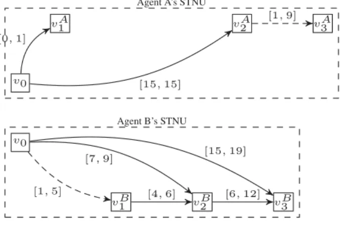
Objective functions Our method can optimize the set of local STNUs by maximizing objective functionfopt =P_i<j(uij− lij). Many other metrics can be used. For example, Fig 10 shows the lo-cal STNUs obtained when minimizing the latest execution time of the last time-point, to finish the mission as soon as possible (mini-mization offopt = maxiu0i). With this new objective function, the maximum mission completion time is reduced from29 time units to 24 time units. v0 v0 vA₁ [0, 1] vA₂ [15, 15] vA₃ [1, 9] vB₁ [1, 5] vB₂ [4, 6] [7, 9] vB₃ [6, 12] [15, 19] Agent A’s STNU

Agent B’s STNU

Figure 10. Mission duration optimization

Objective functions can also be used to balance the flexibility of solutions between agents, in order to avoid overly constrained agents. In this case, we define the normalized flexibility metricsf :

∀a ∈ A, f (a) = 1

|VA_| P

vi,vj∈VA(uij− lij). The corresponding objective function to maximize is thenfopt = mina∈Af (a). This is particularly useful when the number of agents is high, since in this case the maximum global flexibility can often be reached by con-straining as much as possible an unique agent. Another option can be to keep the initial objective function and constrain the problem such that each agent achieves a minimal thresholdt of normalized flexibility:∀a ∈ A, f (a) ≥ t.

5

Experiments

Running Times We tested our MIP approach using the CPLEX solver on500 instances of randomly-generated MaSTNUs, ranging homogeneously from10 to 40 nodes. All experiments were run on 3.0GHz Intel cores and 4GB memory. Finding the optimal solution to the MIP problem typically takes between0.2 seconds for the 6-nodes example used in this paper, and1200 seconds for a 4-agents and40-nodes example containing 4 external contingent links and 10 external requirement links. However, in this last case a first solution, that strictly improves the solution found by removing external con-tingent links, is found in80 seconds, at the expense of a drop in the flexibility of75% compared to the optimal solution.

It must be noted that our current implementation of DC for lo-cal STNU (section2.4) is based on the O(N5_{)-time DC-checking} techniques from [9], and is the primary cause of the scalability per-formances. A more efficient algorithm inO(N4_{)-time can be found} in [6], however this algorithm is more complex to translate into a MIP formalism and is beyond the scope of this paper.

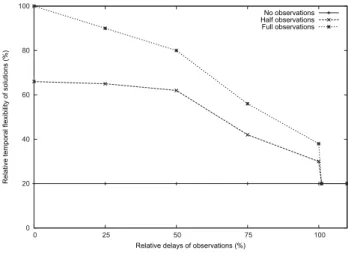
Impact of Observations on Temporal Flexibility For the sake of consistency with real life applications vocabulary, in the remainder of this paper we will refer to external contingent links as observations.

We want to measure the improvements made by our method on the ”quality” of resulting execution strategies. To this end, we define the Relative temporal flexibility of a solution as being the ratio of the value of the objective function of solution to the value of the objective function of the corresponding STNU:

Relative Temporal Flexibility=fopt(M aST N U )

fopt(ST N U ) .

This metric gives us a strong indicator of the ”quality” of a solution compared to best and worst cases. At100% it means the solution is as much flexible as the corresponding STNU, at0% it means that the solution found is totally rigid with no tolerance for execution error.

We also assume that external contingent links take values in[0, x], i.e observations of events by other agents are made withinx unit of times. We comparex to the temporal flexibility of external require-ment links in order to obtain the relative delay of observations:

Relative delay of observations=|E_|CXX|_|· P

(vi,vj )∈CX(uij)

P

(vi,vj )∈EX(uij−lij).

This ratio measure the ”quality” of observations (lower ratio means better quality), which may be translated as cost in real ap-plications.

Fig 11 shows the impact of the number of observations (i.e number of external contingent links) and their quality (i.e their immediacy) on the relative flexibility of the solution found by our method. The parameters of the generated MaSTNUs are as follow:4 agents of 5 nodes each,4 external requirement links (connecting two randomly-chosen nodes from distinct agents). The number of internal require-ment (resp. contigent) links for each agent were randomly drawn from4 to 6 (resp. from 0 to 2). Additional nodes and external con-tingent links, representing observations, were then added depending on the experiments.

Each point on a curve represents the mean of the relative flexibility of the solution found over10 MaSTNUs randomly-generated with the corresponding set of parameters. We display the results for two limit cases, the ”Full observations” and the ”No observations” cases, and an intermediary one, the ”Half observations” case.

The ”No observation” curve corresponds to MaSTNUs without any external contingent links:CX = ∅. In this case, agents cannot receive any informations during execution, so the flexibility of the solution is minimal: agents must agree on a rigid schedule before

0 20 40 60 80 100 0 25 50 75 100

Relative temporal flexibility of solutions (%)

Relative delays of observations (%)

No observations Half observations Full observations

Figure 11. Influence of numbers of observations and delays

execution start. This threshold depends on the MaSTNUs considered, other MaSTNUs may have lower or higher relative flexibility than the 20% reported in our experiments in case of absence of observations. The ”Full observations” curve corresponds to MaSTNUs wherein each event is observed by each other agent:∀v ∈ V, ∀a ∈ A, a += owner(v), ∃w ∈ Va

s.t.(v, w) ∈ CX. In the extreme case with no delays of observation, the resulting solution has the same quality than if the MaSTNU were considered as a STNU. In the opposite extreme case with high delays of observation, no useful informations can be received from the observations, and the agents must act on their own as in the no observation case.

The ”Half observations” curve corresponds to MaSTNUs identi-cal to the ”Full observations” set, except half of vertices inV are not observed by any other agent. The quality of the solution actually depends on which vertices are observed: for instance observations of external vertices are more likely to be useful than observations of internal vertices.

Higher numbers of observations lead to higher flexibility of solu-tions, at the expense of increased computational costs and potentially increased workload during the mission if the observations were not initially scheduled.

6

Conclusion

Dynamic controllability is an important property for temporal plans with uncertainty as it improves the odds of success of a mission. In this paper we showed how to handle uncertain temporal constraints in multi-agent temporal plans thanks to Multi-agent Simple Tempo-ral Network with Uncertainty, and how to use a MIP model to get executable plans which are dispatched between the agents. There are several future work directions for improving the management of MaSTNU, such as solving the MIP incrementally to repair infeasi-ble MaSTNUs by adding observations one by one while optimizing computation times, or distributing the MIP solving process in order to reoptimize temporal plans during the mission, or taking into ac-count the existence of communication rendez-vous [8].

REFERENCES

[1] James C. Boerkoel, L´eon Planken, Ronald Wilcox, and Julie A. Shah, ‘Distributed Algorithms for Incrementally Maintaining Multiagent Sim-ple Temporal Networks’, in Int. Conf. on Automated Planning and Scheduling (ICAPS), Rome, Italy, (2013).

[2] Guillaume Casanova, C´edric Pralet, and Charles Lesire, ‘Managing dy-namic multi-agent simple temporal network’, in Proceedings of the 2015 International Conference on Autonomous Agents and Multiagent Sys-tems (AAMAS), pp. 1171–1179, Istanbul, Turkey, (2015).

[3] Jing Cui, Peng Yu, Cheng Fang, Patrik Haslum, and Brian C. Williams, ‘Optimising bounds in simple temporal networks with uncertainty un-der dynamic controllability constraints’, in Proceedings of the Twenty-Fifth International Conference on Automated Planning and Scheduling (ICAPS), pp. 52–60, Jerusalem, Israel, (2015).

[4] Rina Dechter, Itay Meiri, and Judea Pearl, ‘Temporal Constraint Net-works’, Artificial Intelligence, 49(1-3), 61–95, (1991).

[5] Luke Hunsberger, ‘Efficient execution of dynamically controllable sim-ple temporal networks with uncertainty’, Acta Informatica, 52(8), 1–59, (2015).

[6] Paul Morris, ‘A structural characterization of temporal dynamic control-lability’, in Principles and Practice of Constraint Programming (CP), pp. 375–389, Nantes, France, (2006).

[7] Paul Morris, ‘Dynamic controllability and dispatchability relationships’, in Integration of AI and OR Techniques in Constraint Programming -11th International Conference (CPAIOR), pp. 464–479, Cork, Ireland, (2014).

[8] Paul H. Morris and Nicola Muscettola, ‘Managing temporal uncertainty through waypoint controllability’, in Proceedings of the Sixteenth Inter-national Joint Conference on Artificial Intelligence (IJCAI), pp. 1253– 1258, Stockholm, Sweden, (1999).

[9] Paul H. Morris, Nicola Muscettola, and Thierry Vidal, ‘Dynamic Con-trol Of Plans With Temporal Uncertainty’, in Int. Joint Conference on Artificial Intelligence (IJCAI), Seattle, WA, USA, (2001).