Optimal GPS/GALILEO GBAS methodologies with an application to troposphere

DOCTORAT DE L'UNIVERSITÉ DE TOULOUSE

Délivré par :

Institut National Polytechnique de Toulouse (INP Toulouse)

Discipline ou spécialité :

Signal, Image, Acoustique et Optimisation

Présentée et soutenue par :

Mme ALIZE GUILBERT

le vendredi 1 juillet 2016

Titre :

Unité de recherche :

Ecole doctorale :

OPTIMAL GPS/GALILEO GBAS METHODOLOGIES WITH AN

APPLICATION TO TROPOSPHERE

Mathématiques, Informatique, Télécommunications de Toulouse (MITT)

Laboratoire de Télécommunications (TELECOM-ENAC)

Directeur(s) de Thèse :

M. CHRISTOPHE MACABIAU

M. CARL MILNER

Rapporteurs :

M. BERND EISSFELLER, UNIVERSITAT DER BUNDESWEHR MUNICH

M. FRANK VAN GRAAS, OHIO UNIVERSITY ATHENS

Membre(s) du jury :

1

M. BERND EISSFELLER, UNIVERSITAT DER BUNDESWEHR MUNICH, Président

2

M. CARL MILNER, ECOLE NATIONALE DE L'AVIATION CIVILE, Membre

1

In the Civil Aviation domain, research activities aim to improve airspace capacity and efficiency whilst also tightening safety targets and enabling new more stringent operations. This is achieved through the implementation of new Communications, Navigation, Surveillance and Air Traffic Management (CNS/ATM) technologies and processes. In the navigation domain, these goals are met by improving performance of existing services whilst also expanding the services provided through the development of new Navigation Aids (Navaids) or by defining new operations with existing systems. One such developmental axe for enabling expansion towards new such operations is the provision of safer, more reliable approach and landing operations in all weather conditions.

The Global Navigation Satellite System (GNSS) has been identified as a key technology in providing navigation services to civil aviation users [1] [2] thanks to its global coverage and accuracy in relation to conventional Navaids. This global trend can be observed in the fitting of new civil aviation aircraft since a majority of them are now equipped with GNSS receivers. The GNSS concept includes the provision of an integrity monitoring function by an augmentation system to the core constellations. This is needed to meet the required performance metrics of accuracy, integrity, continuity and availability which cannot be met by the stand-alone constellations. Three such augmentation systems have been developed within civil aviation: the GBAS (Ground Based Augmentation System), the SBAS (Satellite Based Augmentation System) and the ABAS (Aircraft Based Augmentation System).

The Ground Based Augmentation System (GBAS) is currently standardized by the ICAO to provide precision approach navigation services down to Category I using the GPS or GLONASS constellations [3]. Research and standardisation activities are on-going with the objective to extend the GBAS concept to support Category II/III precision approach operations with a single protected signal (GPS L1 C/A), however some difficulties have arisen regarding ionospheric monitoring that threaten to limit availability of this solution.

With the deployment of Galileo and BeiDou alongside the modernization of GPS and GLONASS, it is envisaged that the GNSS future will be multi-constellation (MC) and multi-frequency (MF). European research activities within the SESAR program have focused on the use of GPS and Galileo. The service commitments for this last constellation is expected to be in place in the medium term. The use of two protected frequency bands enables the mitigation of ionospheric errors at the expense of multipath and noise inflation, whilst the improved geometry of two constellations may be used to counter this resulting inflation and enable Cat II/III for worse performing aircraft. Therefore the MC/MF GBAS concept should lead to increased availability, stronger robustness to unintentional interference (due to the use of two protected frequency bands), better ground

segment monitoring capabilities, better modelling of atmospheric effects and improved measurement accuracy from modernized signals. However, several challenges and key issues must be resolved before the potential benefits may be realized.

This PhD has addressed two key topics relating to GBAS, the provision of corrections data within the MC/MF GBAS concept and the impact of tropospheric ranging biases on both the SC/SF and MC/MF GBAS concepts. Due to the tight constraints on GBAS ground to air communications link, the VHF Data Broadcast (VDB) unit, a novel approach is needed when expanding to a MC/MF corrections service [4]. One of the proposals discussed in the PhD project for an updated GBAS VDB message structure is to separate message types for corrections with different transmission rates. Furthermore, This PhD argues that atmospheric modelling with regards to the troposphere has been neglected in light of the ionospheric monitoring difficulties and must be revisited for both nominal and anomalous scenarios. The thesis focuses on how to compute the worst case differential tropospheric delay offline in order to characterize the threat model before extending previous work on bounding this threat in order to protect the airborne GBAS user.

This previous work led by Ohio University for assessing differential tropospheric delays [5] [6] [7] is based on GPS data collection which is inherently subject to undersampling. Furthermore, the bounding methodology was constrained by restricting the scope to SF GPS GBAS and an already defined data message format. In the scope of MC/MF GBAS development, an alternative approach was needed. Therefore, in this PhD project, Numerical Weather Models (NWMs) are used to assess fully the worst case horizontal differential range component of the troposphere (differential tropospheric delay between aircraft and ground assuming aircraft and ground are at the same altitude). An innovative worst case horizontal differential range tropospheric gradient search methodology is used to determine the induced differential ranging biases impacting aircraft performing Cat II/III precision approaches with GBAS. This provides as an output a worst case differential ranging bias as a function of elevation for two European regions (low-elevation coastal and high-elevation mountainous). The range vertical differential component (differential tropospheric delay between aircraft and ground assuming aircraft and ground are not at the same altitude but are at the same latitude and longitude) is also modelled by statistical analysis by comparing the truth data to the GBAS standardized model for vertical tropospheric correction up to the height of the aircraft. A model of the total uncorrected differential ranging bias is generated which must be incorporated within the nominal GBAS protection levels.

In order to bound the impact of the troposphere on the positioning error and by maintaining the goal of low data transmission, different solutions have been developed which remain conservative by assuming that ranging biases conspire in the worst possible way. Through these techniques, in order to protect the user against tropospheric ranging biases, it has been shown that a minimum of 3 parameters may be used to characterize a region’s model.

The main contributions of this thesis are firstly the development of an optimal processing scheme for meeting Cat II/III performance requirements with the MC/MF GBAS trough the derivation of the error budget degradation

when using lower frequency corrections than the current GBAS message correction rate of 2Hz, and the validation of these theoretical analysis with real data. Other contributions deal with the determination and bounding of differential tropospheric ranging biases in the horizontal and vertical directions. Finally, other contributions include the validation of the differential tropospheric ranging biases computation, and the comparison of tropospheric gradients between U.S. data and European data as well as between low relief and high relief regions.

R

ESUME

Dans le domaine de l’Aviation Civile, les motivations de recherches sont souvent guidées par la volonté d’améliorer la capacité et l’efficacité de l’espace aérien grâce à la modernisation des moyens de navigation aérienne existants et à l’ajout de nouvelles infrastructures. Ces buts peuvent être atteints en développant les services qui permettent des opérations d’approche et d’atterrissage plus robustes et plus fiables quels que soient le lieu et les conditions météorologiques.

La navigation par satellite, grâce au Global Navigation Satellite System (GNSS), a été reconnue comme un moyen performant de fournir des services de navigation aérienne [1] [2]. Depuis quelques années, les systèmes de navigation par satellites sont devenus des moyens de navigation de référence grâce à leur couverture mondiale et à leur précision. En particulier, ce système de navigation est utilisé en aviation civile à bord des avions dont la majorité est équipé de récepteurs GNSS. Le concept du GNSS requiert l’utilisation de moyen d’augmentations pour fournir une fonction de contrôle d’intégrité. Cet appui est nécessaire au vu des exigences [1] concernant la précision, l’intégrité, la disponibilité et la continuité des systèmes GNSS surtout dans les applications critiques de type aviation civile. Trois moyens d’augmentation ont alors été développés: le GBAS (Ground Based Augmentation System), le SBAS (Satellite Based Augmentation System) et le ABAS (Aircraft Based Augmentation System).

Le GBAS est actuellement standardisé par l’OACI pour fournir un service de navigation incluant les approches de précision allant jusqu’à la catégorie I incluse, en utilisant les constellations GPS ou GLONASS [3]. Des travaux de recherches et de développement sont en cours pour permettre d’étendre ce service jusqu’à catégorie II/III avec un seul signal protégé (GPS L1 C/A). Cependant des contraintes limitant la disponibilité de cette solution sont apparues lors de la surveillance de la ionosphère.

Grâce à la modernisation du GPS et GLONASS et à la future implémentation des constellations Galileo et Beidou, les futurs GNSS utilisant de multiples constellations et de multiples fréquences (MC/MF) sont étudiés. En Europe, les activités de recherches dans le cadre du projet SESAR se sont appuyées sur la constellation GPS et sur la disponibilité future de la constellation Galileo. L’utilisation de deux bandes de fréquences protégées permet la réduction des retards ionosphériques tout en augmentant l’impact du bruit et des multi-trajets. Cependant l’amélioration de la géométrie des satellites, grâce aux deux constellations, peut compenser cette augmentation et permettre de réaliser des approches de précision de catégorie II/III. C’est pour cela que le MC/MF GBAS devrait permettre de nombreuses améliorations telles que l’augmentation de la disponibilité du système, la meilleure robustesse face aux interférences, un meilleur modèle des retards atmosphériques et une meilleure précision due aux nouveaux signaux de meilleure qualité. Cependant, de nombreux challenges et problèmes doivent être résolus avant d’atteindre les bénéfices potentiels.

Dans ce travail de thèse, deux principaux sujets en rapport avec le GBAS ont été traités, la transmission des données de corrections dans le contexte du MC/MF GBAS et l’impact des biais de mesures troposphériques dans le cadre du SC/SF GBAS et du MC/MF GBAS. Dû aux strictes contraintes portant sur le format des messages transmis à l’utilisateur via l’unité de VHF (Very High Frequency) Data Broadcast (VDB) [4], une nouvelle approche est nécessaire pour permettre l’élaboration du MC/MF GBAS. Une des solutions proposée dans cette thèse est de transmettre les corrections et les données d’intégrité à l’utilisateur dans des messages séparés à des fréquences différentes. De plus ce travail de thèse remet en question la modélisation de l’atmosphère. En effet, au vue de la difficulté de surveiller les retards ionosphériques, ceux relatifs à la troposphère furent en partie négligés et doivent être réévalués aussi bien dans des conditions nominales que non-nominales. Cette thèse se concentre d’abord sur les moyens de calculer le pire gradient troposphérique pour caractériser la menace troposphérique avant de développer les précédents travaux pour borner cette menace dans le but de protéger l’utilisateur.

Les précédentes études faites par l’Université d’Ohio pour traiter les retards troposphérique différentiels [5] [6] [7] sont basées sur la collecte de données GPS qui est intrinsèquement liée à du sous-échantillonnage. De plus, dans le cadre du SF GPS GBAS, la méthode pour borner l’erreur fut contrainte par le format du message transmis. En vue du futur MC/MF GBAS, une nouvelle approche s’est avérée nécessaire. C’est pour cela que dans ce projet de thèse, des modèles météorologiques numériques (NWMs) sont utilisés pour estimer intégralement la composante horizontale du pire retard différentiel troposphérique (retard différentiel dû à la décorrelation horizontale entre l’avion et la station sol). Une méthode innovante pour rechercher les pires retards différentiels troposphériques horizontaux est utilisée pour déterminer les biais de mesures qu’ils induisent impactant les avions visant une approche de Cat II/III avec le GBAS. Un modèle de ces pires biais de mesure troposphériques différentiels horizontaux dépendant de l’élévation des satellites pour 2 régions européennes (une région côtière à bas-relief et une région montagneuse à haut relief) est alors développé. La composante verticale du pire retard différentiel troposphérique (retard différentiel dû à la différence d’altitudes entre l’avion et la station sol) est aussi modélisée grâce à une étude statistique qui compare les données réelles au modèle standard établi pour le GBAS. Un modèle du biais de mesure différentiel total non corrigé est développé et doit être introduit dans le calcul des niveaux de protections sous des conditions nominales.

Pour borner l’impact de la troposphère sur l’erreur de position tout en se focalisant sur le souhait d’avoir un nombre de données transmises à l’utilisateur faible, différentes solutions ont été développées. Elles restent conservatives en supposant que les biais de mesures se combinent pour engendrer la pire erreur de position verticale. Avec ces méthodes, au minimum 3 paramètres, définis selon leur région géographique d’utilisation, doivent être transmis à l’utilisateur pour le protéger contre ces biais de mesures troposphériques.

Les principales contributions de cette thèse sont le développement d’un modèle optimal de traitements pour répondre aux exigences liées à la Cat II/III d’approche avec le MC/MF GBAS. Ceci a été effectué tout d’abord grâce à l’analyse théorique de la possibilité d’avoir des messages transmis à une fréquence plus faible que celle standardisée actuellement à 2 Hz puis par la validation de cette possibilité grâce à l’analyse de données réelles.

Ensuite, les autres apports de cette thèse portent sur les solutions permettant de déterminer et de borner les biais de mesures troposphériques différentiels dans les directions horizontales et verticales. Enfin, d’autres contributions incluent la validation du calcul des biais troposphériques et la comparaison entre les gradients troposphériques apparaissant dans les données américaines et européennes pour une région côtière à bas-relief et une région montagneuse à haut bas-relief.

A

CKNOLEDGEMENTS

Tout d’abord, je souhaiterais particulièrement remercier mon directeur de thèse Christophe Macabiau et mon co-directeur de thèse Carl Milner pour leur disponibilité, leur temps, leur patience et leur gentillesse. C’est en grande partie grâce à eux et à leur expertise dans le domaine du GNSS que j’ai pu réussir à valider ce doctorat.

Je voudrais remercier ensuite la Commission Européenne et l’ENAC pour avoir financé mes travaux de thèse au sein du projet SESAR ainsi que toutes les entreprises partenaires de ce projet.

Mes plus vifs remerciements vont également à Henk Veerman du NLR pour m’avoir aidé à travailler sur la Troposphère et de m’avoir permis d’exploiter les données Harmonie de KNMI, ainsi que Météo France avec Pierre Brousseau pour m’avoir fourni les données AROME et pour m’avoir expliqué comment les modèles météorologiques avaient été développés.

I would like to thank Pr. Bernd Eissfeller and Pr. Frank Van Graas for their reviews and for having attended my PhD defense.

Merci aussi à Pierre Ladoux pour son aide et sa disponibilité durant ce projet SESAR et pour avoir accepté d’être membre de mon jury de thèse.

Ensuite, je dois en partie ma réussite de ce doctorat à mes collègues du laboratoire SIGNAV et particulièrement Giuseppe Rotondo qui a partagé mon bureau et qui m’a beaucoup aidé pendant ces 3 ans, Paul Thevenon et Jeremy Vezinet pour leurs précieux conseils, leurs analyses et leurs corrections tout au long de ma thèse.

Enfin, je n’aurais pas pu mener à bien mes travaux de thèse sans le soutien de mes parents Fouzia Bouchareb et Bruno Guilbert, de mon « frérot » Guillaume Guilbert et des autres membres de ma famille. Ils m’ont poussé à faire cette thèse et je leur dois tout.

Je n’oublie pas mes amis qui ont su me soutenir, me supporter, me motiver, me changer les idées tous les jours pendant ces 3 dernières années. Un énorme merci à mes « copines » Charlotte Blanc, Aurélie Deloeil qui étaient présentes lors de ma soutenance.

T

ABLE OF

C

ONTENTS

Chapter 1 : Introduction...25

1.1 Background and Motivation...25

1.1.1 Background ... 25

1.1.2 SESAR Project ... 25

1.1.3 Ground Based Augmentation System *1 _{... 27}

1.2 Objectives and Contributions ... 27

1.2.1 Objectives ... 27

1.2.2 Original Contributions ... 30

1.3 Dissertation Organization...31

Chapter 2 : Navigation Performance Requirements for Civil Aviation...33

2.1 Civil Aviation Authorities...33

2.1.1 International Civil Aviation Organization (ICAO) ... 33

2.1.2 RTCA, Inc. ... 33

2.1.3 EUROCAE ... 34

2.1.4 FAA and EASA ... 34

2.2 Phases of Flight...34

2.2.1 Categories of flight phases ... 35

2.2.2 Approaches ... 35

2.3 Performance Based Navigation – PBN...37

2.4 Operational Criteria for Navigation Performance...39

2.4.1 Accuracy ... 39

2.4.2 Availability ... 39

2.4.3 Continuity ... 39

2.4.4 Integrity ... 39

2.5 Annex 10 [3] SIS Performance Requirements ... 40

2.5.1 Existing requirements... 40

2.5.2 CAT II/III ... 43

Chapter 3 : GNSS Processing...45

3.1 The Civil Aviation GNSS Concept....... 45

3.1.1 Introduction ... 45

3.1.2 Principle of Satellite Positioning [29] ... 46

3.1.3 Planning of GNSS implementation in Civil Aviation ... 47

3.1.4 Differential GNSS in Civil Aviation ... 51

3.2.1 Raw Measurements ... 60

3.2.2 Measurement Error Model ... 61

3.2.3 Measurement Processing *4 _{... 72}

3.3 Navigation Solution ... 102

3.3.1 Position Computation... 103

3.3.2 Integrity Monitoring ... 108

3.4 Conclusions ... 123

Chapter 4 : Optimal Processing Models/Options for MC/MF GBAS ... 125

4.1 Introduction ... 125

4.2 Error Model ... 126

4.2.1 Error Modelling ... 126

4.2.2 GBAS Tropospheric Error ... 137

4.3 Evolution of Corrections Computation ... 139

4.3.1 Presentation ... 139

4.3.2 RRC Analysis ... 141

4.3.3 PseudoRange Performances Analysis... 144

4.4 Performance Benefits ... 148

4.4.1 Trade-offs ... 148

4.4.2 Conclusions ... 148

Chapter 5 : Anomalous Troposphere Modelling for GBAS ... 151

5.1 Introduction ... 151

5.2 Meteorological Modelling ... 152

5.2.1 Weather Wall Model ... 153

5.2.2 Numerical Weather Model ... 156

5.3 Tropospheric Delay Modelling and Computation ... 164

5.3.1 Total Refractive Index ... 164

5.3.2 2D Empirical Model ... 166

5.3.3 3D layered Model ... 167

5.4 Horizontal Differential Tropospheric Delay ... 171

5.4.1 Zenith Tropospheric Delay (Step A) ... 172

5.4.2 Differential Zenith Tropospheric Delay (Step B) ... 173

5.4.3 Worst Direction for Differential Zenith Tropospheric Delay (Step C)... 173

5.4.4 Worst Differential Tropospheric Delay (Step D) ... 174

5.4.5 Accuracy of this methodology with NWM ... 181

5.5 Vertical Component Modelling ... 184

5.5.1 GAST C/D Tropospheric Correction ... 184

5.5.3 Conclusions ... 196

Chapter 6 : Anomalous Troposphere Bounding ... 197

6.1 Introduction ... 197

6.2 Existing GAST C/D Methodology ... 197

6.2.1 Introduction ... 197

6.2.2 Overbounding and Sigma Inflation Concepts ... 199

6.2.3 Protection Levels ... 202

6.2.4 Conclusions ... 205

6.3 Innovative Methodology ... 206

6.3.1 Bias-Parameter Transmission Methodologies... 206

6.3.2 Ionosphere-Free case ... 219

6.4 Numerical Weather Model Based Methodology ... 221

6.4.1 Worst Horizontal Differential Tropospheric Delay ... 221

6.4.2 Vertical Ranging Biases ... 230

6.4.3 Conspiring Ranging Biases Assumption Validation ... 233

6.5 Conclusions and Recommendations ... 234

Chapter 7 : Conclusions and Future Work ... 237

7.1 Conclusions ... 237

7.2 Perspectives for future work ... 239

References 241 Appendix A : Other scenarios for computing Anomalous Tropospheric delays ... 249

A.1 Ohio Assumption for Number of Visible Satellites ... 249

A.1.1 𝑫𝒕𝒉= 5km ... 249

A.1.2 𝑫𝒕𝒉 = 10km ... 250

A.2 Other points along the Approach for Seattle Airport with 𝑫𝒕𝒉=5 km ... 252

A.2.1 D=20NM ... 253

A.2.2 D=10NM ... 254

A.2.3 H=100ft ... 255

A.2.4 H=0ft ... 256

A.3 Seattle airport with 𝑫𝒕𝒉 =10 km ... 256

Appendix B : Different Airport Locations ... 260

B.1 LAT 0 ... 261 B.1.1 Dth=5km ... 261 B.1.2 Dth=10km ... 263 B.2 Miami ... 265 B.2.1 Dth=5km ... 265 B.2.2 Dth=10km ... 267

B.3 Anchorage ... 269

B.3.1 Dth=5km ... 269

B.3.2 Dth=10km ... 271

Appendix C : Other I-free scenarios ... 274

C.1 Seattle ... 274 C.1.1 Dth=5km ... 274 C.1.2 Dth=10km ... 275 C.2 LAT 0 ... 279 C.2.1 Dth=5km ... 279 C.2.2 Dth=10km ... 282 C.3 Miami ... 285 C.3.1 Dth=5km ... 285 C.3.2 Dth=10km ... 288 C.4 Anchorage ... 291 C.4.1 Dth=5km ... 291 C.4.2 Dth=10km ... 294

T

ABLE OF FIGURES

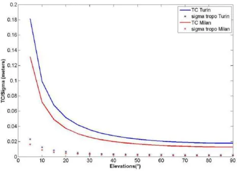
Figure 1-GBAS Troposphere Delay Paths ________________________________________________________ 30 Figure 2-Phases of flight and GNSS augmentations [24] ____________________________________________ 36 Figure 3-Total System Error [17] _______________________________________________________________ 38 Figure 4-ILS Look-Alike Method ________________________________________________________________ 43 Figure 5-Autoland Method ___________________________________________________________________ 44 Figure 6-DGNSS principle _____________________________________________________________________ 51 Figure 7-GBAS volume Coverage [1] ____________________________________________________________ 54 Figure 8-GBAS architecture ___________________________________________________________________ 55 Figure 9-GBAS processing scheme _____________________________________________________________ 60 Figure 10-Impact of in phase multipath on the output of the correlator _______________________________ 67 Figure 11-Impact of multipath on discriminator output_____________________________________________ 68 Figure 12-Raw and smoothed tracking error [68] _________________________________________________ 68 Figure 13-Differential Measurement Processing __________________________________________________ 73 Figure 14-Carrier Smoothing Block Diagram _____________________________________________________ 73 Figure 15-Differential Positioning Architecture ___________________________________________________ 81 Figure 16-Differential Positioning Architecture with Range-Rate Correction [47] ________________________ 82 Figure 17-PRC computation ___________________________________________________________________ 82 Figure 18-Pseudorange Processing [41] _________________________________________________________ 84 Figure 19-Determination of TC and sigma tropo parameters ________________________________________ 85 Figure 20-TC and sigma tropo for Schiphol location ________________________________________________ 86 Figure 21-Tropospheric Correction and Sigma tropo at Turin/Milan ___________________________________ 87 Figure 22-Error budget for Galileo and GPS new signals [83] ________________________________________ 90 Figure 23-Velocity profile Model [88] ___________________________________________________________ 95 Figure 24-Format of a GBAS message block [78] __________________________________________________ 99 Figure 25-Format of Message type 1 [78] _______________________________________________________ 100 Figure 26-Format of the message type 2 [78]____________________________________________________ 101 Figure 27-Format of the additional data block 3 [75] _____________________________________________ 101 Figure 28-Format of the message type 11 ______________________________________________________ 102 Figure 29-Relationship between alert and protection levels: a) available integrity monitoring system, b)

unavailable integrity monitoring system [63] ____________________________________________________ 110 Figure 30-Continuity and Integrity Decision Process ______________________________________________ 111 Figure 31-SBAS SIS integrity Tree _____________________________________________________________ 112 Figure 32-GBAS Integrity tree ________________________________________________________________ 113 Figure 33-GAST D Aircraft Architecture [16] _____________________________________________________ 119 Figure 34-DSIGMA principle _________________________________________________________________ 120 Figure 35-Standard deviation of the Residual Satellite Clock Error over time [51] _______________________ 130 Figure 36-Impact of elevation and t_AZ on the total standard deviation for GPS L1C/A with τ=100s ________ 133 Figure 37-Impact of elevation and t_AZ on the total standard deviation for GPS L1-L5 DFree with τ=100s ___ 135 Figure 38-Impact of elevation and t_AZ on the total standard deviation for GPS L1-L5 DFree with τ=30s ____ 135 Figure 39-Impact of elevation and t_AZ on the total standard deviation for GPS L1-L5 IFree with τ=100s ____ 137 Figure 40-PRC and RRC over time _____________________________________________________________ 140 Figure 41-Std for 100s smoothed RRC __________________________________________________________ 141 Figure 42-Std for 30s smoothed RRC ___________________________________________________________ 141 Figure 43-Distribution of RRC for all satellites for MT1 (100s) _______________________________________ 142 Figure 44-Distribution of RRC for all satellites for MT11 (30s) _______________________________________ 142 Figure 45-RRC over 1minute _________________________________________________________________ 143

Figure 46-Standard deviation of RRC for MT1 (blue) and MT11 (red) _________________________________ 143 Figure 47-100s Smoothed Error Degradation with Update Period ___________________________________ 144 Figure 48-30s Smoothed Error Degradation with Update Period ____________________________________ 144 Figure 49-D-free Smoothed Error Degradation with Update Period with τ=100s ________________________ 145 Figure 50-D-free Smoothed Error Degradation with Update Period with τ=30s _________________________ 145 Figure 51-I-free Smoothed Error Degradation with Update Period ___________________________________ 146 Figure 52-Standard deviation of ∆𝑷𝑹𝑪 for different time of extrapolation for MT1 _____________________ 147 Figure 53-Standard deviation of ∆𝑷𝑹𝑪 for different time of extrapolation for MT11 ____________________ 147 Figure 54-Weather Wall Model to the right of the Ground Station ___________________________________ 153 Figure 55-Determination of σ_vig for 5° Elevation ________________________________________________ 155 Figure 56-Determination of σ_vig for 90° Elevation _______________________________________________ 155 Figure 57-Sensors for NWM [119] _____________________________________________________________ 156 Figure 58-Area of study with Arome – Source : Google Earth V7.1.5.1557- 10/04/2013 __________________ 157 Figure 59-Surface height of Arome domain _____________________________________________________ 158 Figure 60-12 Height levels ___________________________________________________________________ 158 Figure 61-Height levels of NWM ______________________________________________________________ 159 Figure 62-Pressure levels of NWM ____________________________________________________________ 159 Figure 63-Temperature levels of NWM _________________________________________________________ 160 Figure 64-RH levels for NWM ________________________________________________________________ 160 Figure 65-Vertical Profiles (over pressure coordinates in hPa) for Height Parameter in meters ____________ 161 Figure 66-Vertical Profiles (over pressure coordinates in hPa) for Temperature Parameter in K ____________ 161 Figure 67-Vertical Profiles (over pressure coordinates in hPa) for RH Parameter in % ____________________ 162 Figure 68-Harmonie domain –Source: Google Earth V7.1.5.1557- 10/04/2013 _________________________ 163 Figure 69-Surface height of Harmonie domain ___________________________________________________ 163 Figure 70-Illustration of a troposphere split into layers ____________________________________________ 165 Figure 71-(a) -Vertical Interpolation - (b) Additional Horizontal Interpolation __________________________ 168 Figure 72-Interpolation of Heights ____________________________________________________________ 168 Figure 73-Interpolation of Pressures ___________________________________________________________ 169 Figure 74-Interpolation of Temperatures _______________________________________________________ 169 Figure 75-Interpolation of RH ________________________________________________________________ 170 Figure 76-Interpolation of Refractivities ________________________________________________________ 171 Figure 77-ZTD computed with Harmonie data ___________________________________________________ 172 Figure 78-Definition of the 10 segments of study _________________________________________________ 173 Figure 79-Searching for worst azimuthal direction _______________________________________________ 174 Figure 80-Segment translation _______________________________________________________________ 175 Figure 81-Finding the worst case for Differential Range Tropospheric Delay ___________________________ 175 Figure 82-Differential range Tropospheric Delay _________________________________________________ 176 Figure 83-Wall model with different parameterizations ___________________________________________ 177 Figure 84-Max differential range tropo delay for Harmonie ________________________________________ 178 Figure 85-Max differential range tropo delay for Arome ___________________________________________ 178 Figure 86-Max differential range tropo delay for Arome from 10° ___________________________________ 179 Figure 87-Bounding Curves for each model stating at 5° ___________________________________________ 180 Figure 88-Bounding Curves for each model stating at 10° __________________________________________ 180 Figure 89-Nd/Nw for A/C ____________________________________________________________________ 181 Figure 90-Nd/Nw for Gnd ___________________________________________________________________ 182 Figure 91-Tropospheric Delay for A/C (left) and Ground (right) _____________________________________ 182 Figure 92-ZTD for Harmonie data at 200ft ______________________________________________________ 185 Figure 93-Difference between TC and ZTD for Harmonie data ______________________________________ 186 Figure 94-ZTD for Arome data at 200ft _________________________________________________________ 187 Figure 95-Difference between TC and ZTD for Arome data _________________________________________ 187 Figure 96-Difference between TC and ZTD for Turin ______________________________________________ 189

Figure 97-Difference between TC and ZTD for Milan ______________________________________________ 190 Figure 98-Difference between TC and ZTD for Schiphol ____________________________________________ 190 Figure 99-STD of (TC-ZTD) over the grid compared to sigma tropo at Turin ____________________________ 191 Figure 100-STD of (TC-ZTD) over the grid compared to sigma tropo at Milan __________________________ 191 Figure 101-STD of (TC-ZTD) over the grid compared to sigma tropo at Schiphol ________________________ 192 Figure 102-Histogram of TC-ZTD over 1 year at Turin _____________________________________________ 192 Figure 103-Histogram of TC-ZTD over 1 year at Milan _____________________________________________ 193 Figure 104-Histogram of TC-ZTD over 2 years at Schiphol __________________________________________ 193 Figure 105-TC bias _________________________________________________________________________ 194 Figure 106-Inflated VPL _____________________________________________________________________ 200 Figure 107-VPLs with D_TH=5km for GPS constellation ____________________________________________ 203 Figure 108-VPLs with D_TH=5km for GPS+GAL __________________________________________________ 204 Figure 109-VPLs with D_TH=10km for GPS constellation ___________________________________________ 204 Figure 110-VPLs with D_TH=10km for GPS+GAL _________________________________________________ 205 Figure 111-VPLs with D_TH =5km for GPS constellation only _______________________________________ 208 Figure 112-VPLs with D_TH =5km for GPS + GAL constellations _____________________________________ 209 Figure 113-VPLs with D_TH =5km for GPS constellation only _______________________________________ 210 Figure 114-VPLs with D_TH =5km for GPS and Gal constellations ____________________________________ 210 Figure 115-𝝁𝒎𝒂𝒙with the 2 new methodologies ________________________________________________ 212 Figure 116-VPLs with D_TH =5km for GPS constellation ___________________________________________ 213 Figure 117-VPLs with D_TH=5km for GPS+GAL __________________________________________________ 214 Figure 118-VPLs with D_TH=5km for GPS _______________________________________________________ 215 Figure 119-VPLs with D_TH=5km for GPS+GAL __________________________________________________ 216 Figure 120-Representation of the Worst subset Q ________________________________________________ 217 Figure 121-Representation of the Subset Q and the wall model _____________________________________ 217 Figure 122-VPLs with D_TH=5km for GPS constellation ____________________________________________ 218 Figure 123-VPLs with D_TH=5km for GPS+GAL __________________________________________________ 218 Figure 124-VPLs for I-free case with 100s smoothing constant with D_TH =5km for GPS constellation ______ 219 Figure 125-VPLs for I-free case with 100s smoothing constant with D_TH =5km for GPS/GAL constellations _ 220 Figure 126-VPLs for GPS constellation _________________________________________________________ 223 Figure 127-VPLs for GPS and GAL constellations _________________________________________________ 223 Figure 128-VPLs for GPS with a cut-off angle of 10°_______________________________________________ 224 Figure 129-VPLs for GPS and GAL constellations with a cut off angle of 10° ___________________________ 224 Figure 130-VPL LDP for Arome with GPS/GAL and cut off angle at 10° with Curves C and D _______________ 226 Figure 131-VPLs for GPS constellation _________________________________________________________ 227 Figure 132-VPLs for GPS and GAL constellations _________________________________________________ 227 Figure 133-VPLs I-free for GPS constellation_____________________________________________________ 228 Figure 134-VPLs I-free for GPS and GAL constellation _____________________________________________ 229 Figure 135-VPLs I-free for GPS and GAL constellation with cut off angle at 10° _________________________ 229 Figure 136-VPLs at Schiphol for GPS constellation ________________________________________________ 230 Figure 137-VPLs at Schiphol for GPS+GAL _______________________________________________________ 231 Figure 138-VPLs at Turin and Milan for GPS constellation _________________________________________ 231 Figure 139-VPLs at Turin and Milan for GPS+GAL ________________________________________________ 232 Figure 140-VPLs at Turin and Milan for GPS+GAL with a cut-off angle at 10° __________________________ 232 Figure 141-VPLs for validating conspiring biases assumptions ______________________________________ 233 Figure 142-VPLs Seattle Dth=5km, GPS N=6 _____________________________________________________ 250 Figure 143-VPLs Seattle Dth=5km, GPSand GAL N=12 _____________________________________________ 250 Figure 144-VPLs Seattle Dth=10km, GPS N=6 ____________________________________________________ 251 Figure 145-VPLs Seattle Dth=10km, GPS and GAL N=12 ___________________________________________ 251 Figure 146-VPLs Seattle, D=20NM, Dth=5km, GPS (figure above) and GPS and GAL(figure below)__________ 253 Figure 147-VPLs Seattle, D=10NM, Dth=5km, GPS (figure above) and GPS and GAL(figure below)__________ 254

Figure 148-VPLs Seattle, h=100ft, Dth=5km, GPS (figure above) and GPS and GAL(figure below) __________ 255 Figure 149-VPLs Seattle, h=0ft, Dth=5km, GPS (figure above) and GPS and GAL(figure below) ____________ 256 Figure 150-VPLs Seattle, GPS (left) and the GPS and GAL (right), Dth=10km __________________________ 258 Figure 151-VPLs with WSS methodology for Seattle, GPS (left) and the GPS and GAL (right), Dth=10km ____ 259 Figure 152-VPLs Lat0 GPS (left) and the GPS and GAL (right), Dth=5km _______________________________ 261 Figure 153-VPLs geometry improved Lat0 GPS (left) and the GPS and GAL (right), Dth=5km ______________ 262 Figure 154-VPLs Lat0 GPS (left) and the GPS and GAL (right), Dth=10km _____________________________ 263 Figure 155-VPLs geometry improved, Lat0 GPS (left) and the GPS and GAL (right), Dth=10km ____________ 264 Figure 156-VPLs Miami GPS (left) and the GPS and GAL (right), Dth=5km ____________________________ 265 Figure 157-VPLs Miami geometry improved, GPS (left) and the GPS and GAL (right), Dth=5km ___________ 266 Figure 158-VPLs Miami GPS (left) and the GPS and GAL (right), Dth=10km ___________________________ 267 Figure 159-VPLs Miami geometry improved, GPS (left) and the GPS and GAL (right), Dth=10km __________ 268 Figure 160-VPLs Anchorage GPS (left) and the GPS and GAL (right), Dth=5km _________________________ 269 Figure 161-VPLs Anchorage geometry improved GPS (left) and the GPS and GAL (right), Dth=5km _________ 270 Figure 162-VPLs Anchorage GPS (left) and the GPS and GAL (right), Dth=10km________________________ 271 Figure 163-VPLs Anchorage geometry improved GPS (left) and the GPS and GAL (right), Dth=10km _______ 272 Figure 164-VPLs IF 300s Seattle, GPS (left) and GPS and GAL (right), Dth5km __________________________ 274 Figure 165-VPLs IF 1000s Seattle, GPS (left) and GPS and GAL (right), Dth5km _________________________ 275 Figure 166-VPLs IF 100s Seattle, GPS (left) and GPS and GAL (right), Dth10km _________________________ 276 Figure 167-VPLs IF 300s Seattle, GPS (left) and GPS and GAL (right), Dth10km _________________________ 277 Figure 168-VPLs IF 1000s Seattle, GPS (left) and GPS and GAL (right), Dth10km ________________________ 278 Figure 169-Comparison VPLs IF performance for Seattle ___________________________________________ 279 Figure 170-VPLs IF 100s LAT0, GPS (left) and GPS and GAL (right), Dth5km ____________________________ 280 Figure 171-VPLs IF 300s LAT0, GPS (left) and GPS and GAL (right), Dth5km ____________________________ 281 Figure 172-VPLs IF 1000s LAT0, GPS (left) and GPS and GAL (right), Dth5km ___________________________ 282 Figure 173-VPLs IF 100s LAT0, GPS (left) and GPS and GAL (right), Dth10km ___________________________ 283 Figure 174-VPLs IF 300s LAT0, GPS (left) and GPS and GAL (right), Dth10km ___________________________ 284 Figure 175-VPLs IF 1000s LAT0, GPS (left) and GPS and GAL (right), Dth10km __________________________ 285 Figure 176-VPLs IF 100s Miami, GPS (left) and GPS and GAL (right), Dth5km __________________________ 286 Figure 177-VPLs IF 300s Miami, GPS (left) and GPS and GAL (right), Dth5km __________________________ 287 Figure 178-VPLs IF 1000s Miami, GPS (left) and GPS and GAL (right), Dth5km _________________________ 288 Figure 179-VPLs IF 100s Miami, GPS (left) and GPS and GAL (right), Dth10km _________________________ 289 Figure 180-VPLs IF 300s Miami, GPS (left) and GPS and GAL (right), Dth10km _________________________ 290 Figure 181-VPLs IF 1000s Miami, GPS (left) and GPS and GAL (right), Dth10km ________________________ 291 Figure 182-VPLs IF Anchorage 100s , GPS (left) and GPS and GAL (right), Dth5km ______________________ 292 Figure 183-VPLs IF Anchorage 300s , GPS (left) and GPS and GAL (right), Dth5km ______________________ 293 Figure 184-VPLs IF Anchorage 1000s , GPS (left) and GPS and GAL (right), Dth5km _____________________ 294 Figure 185-VPLs IF Anchorage 100s , GPS (left) and GPS and GAL (right), Dth10km _____________________ 295 Figure 186-VPLs IF Anchorage 300s , GPS (left) and GPS and GAL (right), Dth10km _____________________ 296 Figure 187-VPLs IF Anchorage 1000s , GPS (left) and GPS and GAL (right), Dth10km ____________________ 297

T

ABLE OF

T

ABLES

Table 1 - Decision heights and Visual requirements [23] ____________________________________________ 37 Table 2-SIS performance requirements [1] _______________________________________________________ 41 Table 3-Alert Limits associated to typical operations [1] ____________________________________________ 42 Table 4-SIS Performance Requirements for the various phases of aircraft operation [28] __________________ 44 Table 5-GPS signals for civil aviation ____________________________________________________________ 48 Table 6-Galileo signals for civil aviation _________________________________________________________ 50 Table 7-GBAS service levels [27] _______________________________________________________________ 58 Table 8-GCID classification [27] ________________________________________________________________ 58 Table 9-Comparison between Klobuchar and Nyquist models ________________________________________ 65 Table 10-Parameters for DLL tracking error variance computation ___________________________________ 71 Table 11-Yearly mean values for Schiphol _______________________________________________________ 85 Table 12-Yearly mean values for De Bilt _________________________________________________________ 86 Table 13-Yearly mean values for Turin and Milan _________________________________________________ 86 Table 14-Non-aircraft Elements Accuracy Requirement [27] _________________________________________ 91 Table 15-Proposition for Non-aircraft Elements Accuracy GAST D ____________________________________ 92 Table 16-Airborne Accuracy Designator [27] _____________________________________________________ 92 Table 17-Airframe Multipath Designator [27] ____________________________________________________ 93 Table 18-Residual Ionospheric Uncertainty parameters assumptions [27] ______________________________ 94 Table 19-Airborne speed Profile [88]____________________________________________________________ 95 Table 20-GBAS message types [78] _____________________________________________________________ 99 Table 21-Differential Processing options _______________________________________________________ 125 Table 22 – Percentage of errors done by using NWMs for computing differential range tropospheric delays _ 184 Table 23-Percentage of errors done by using NWMs for computing differential range tropospheric delays up to 200ft ____________________________________________________________________________________ 184 Table 24-Turin, Milan, Schiphol coordinates_____________________________________________________ 188 Table 25-TC and sigma tropo for Turin, Milan and Schiphol locations ________________________________ 189 Table 26-Bias between TC and ZTD ____________________________________________________________ 194 Table 27- 𝝈∆𝒕𝒓 and 𝝈𝒗𝒊𝒈 𝒊𝒏𝒇 for different cases ________________________________________________ 202 Table 28-Airports Coordinates________________________________________________________________ 202 Table 29-Steps according Distances GND-A/C ___________________________________________________ 207 Table 30-Look-up table of 𝝁𝒎𝒂𝒙 _____________________________________________________________ 207 Table 31-Look up table with a variable width of bin ______________________________________________ 209 Table 32-Proposed ADB 6 for MT2 with LUT _____________________________________________________ 211 Table 33-Fitted curves parameters for Wall Model _______________________________________________ 212 Table 34-SF Availabilities ____________________________________________________________________ 215 Table 35-I-free Availabilities _________________________________________________________________ 220 Table 36-Fitted curves parameters for Ohio/ Harmonie / Arome ____________________________________ 222 Table 37-Percentage of the mean difference between VPLs ________________________________________ 225 Table 38-Look up table for AROME data with a variable width of bin_________________________________ 227 Table 39 – Percentage of differences between VPLs with and without vertical biases. ___________________ 233 Table 40-Proposed ADB 6 for MT2 with LDT _____________________________________________________ 235 Table 41-Proposed ADB 6 for MT2 with LDT if DC with a cut off angle at 10° __________________________ 236

20

©SESAR JOINT UNDERTAKING, 2014. Created by AENA, Airbus, DFS, DSNA, ENAC, ENAV, EUROCONTROL, Honeywell, INDRA, NATMIG, Selex, Thales and AT-One for the SESAR Joint Undertaking within the frame of the SESAR Programme co-financed by the EU and

GNSS Global Navigation Satellite System

GBAS Ground Based Augmentation System

ABAS Aircraft Based Augmentation System

SBAS Satellite Based Augmentation System

GPS Global Positioning Service

MC Multi-Constellation

MF Mult-Frequency

SESAR Single European Sky ATM Research

ICAO International Civil Aviation Organisation

SC Single Constellation

SF Single Frequency

VDB VHF Data Broadcast

NWM Numerical Weather Model

U.S. United States

C/A Coarse/Acquisition

VHF Very High Frequency

I-free/IF Ionosphere Free

D-free Divergence Free

CNS Communication Navigation Surveillance

ATM Air Traffic Management

21

WP Work Package

RNP Required Navigation Performance

SSR Secondary Surveillance Radar

RF Radio Frequency

ILS Instrument Landing System

GLS GBAS Landing System

SIS Signal In Space

FAA Federal Aviation Administration

TC Tropospheric Correction

PBN Performance Based Navigation

SARPs Standards and Recommended Practices

NPA Non Precision Approach

APV Approaches with vertical guidance

PA Precision Approach

DH Decision Height

RVR Runway Visual Range

MDA Minimum descent Altitude

MDH Minimum Decision height

DA Decision Altitude

RNAV Area Navigation

TSE Total System Error

PSE Path Steering Error

FTE Flght Technical Error

22

PEE Position Estimation Error

HPL Horizontal Protection Level

VPL Vertical Protection Level

HAL Horizontal Alert Limit

VAL Vertical Alert Limit

LAL Lateral Alert Limit

LPL Lateral Protection Level

TTA Time to Alert

RAIM Receiver Autonomous integrity Monitoring

ARNS Aeronautical Radio Navigation Services

DGNSS Differential GNSS

EGNOS European Geostationary Navigation Overlay Service

LAAS Local Area Augmentation System

WAAS Wide Area Augmentation System

WADGNSS Wide Area DGNSS

GEO Geostationary

ESA European Space Agency

LTP/FTP Landing/Ficticious Threshold Point

GPIP Glide Path Intersection Point

LOC Localizer

MMR Multi-Mode Receiver

GFC GBAS Facility Classification

FAST Facility Approach Service Type

23

APD Approach Performance Designator

AST Active Service Type

SST Selected Service Type

LOS Line of Sight

GGTO GPS to Galileo Time offset

TEC Total Electron Content

STD Slant Tropospheric Delay

CMC Code Minus Carrier

PRC PseudoRange Correction

RRC Range Rate Correction

AD Accuracy Designator

GAD Ground AD

AAD Aircraft AD

PAN Position and Navigation

MT Message Type

PVT Position Velocity Time

LSE Least Square Estimation

FD/FDE Fault Detection/Exclusion

SQM Signal Quality Monitoring

CCD Code Carrier Divergence

DQM Data Quality Monitoring

MDM Measurement Quality Monitoring

MRCC Multiple Receiver Consistency Check

24

BAM Bias Approach Monitor

RRFM Reference Receiver Fault Monitor

DCMC Differential Correction Magnitude Check

RR Reference Receiver

FAS Final Approach Segment

FASVAL FAS Vertical Alert Limit

HPDCM Horizontal Position Differential Correction Magnitude

IGM Iono Gradient Monitor

RH Relative Humidity

P Pressure

T Temperature

MHM Modified Hopfield Model

ZTD Zenith Tropo Delay

SHD Slant Hydrostatic Delay

SWD Slant Wet Dalay

ADB Additional Data Block

GND Ground

A/C Aircraft

LUT Look up Table Transmission

LDT Low Data Transmission

25

1.1 Background and Motivation

1.1.1 Background

Nowadays, most of the civil aviation aircrafts are equipped with Global Navigation Satellite System (GNSS) receivers (90% of aircrafts according the EUROCONTROL Survey [8]) and since it was recognized as a key technology in providing accurate navigation services with a worldwide coverage. This GNSS concept was defined by the International Civil Aviation Organization (ICAO) [1] and is today understood to be composed of the core constellations GPS (Global Positioning System) and GLONASS, the future constellations Galileo and BeiDou constellations implementations, as well as approved augmentations. In view of the stringent civil aviation specifications and requirements defined for the use of GNSS within the CNS/ATM system (Communications, Navigation, and Surveillance / Air Traffic Management), a stand-alone core constellation need augmentations systems for meeting requirements specified by ICAO [1] in terms of accuracy, integrity, availability and continuity. Therefore, several augmentation systems able to monitor GNSS integrity have been developed such as GBAS (Ground Based Augmentation System), SBAS (Satellite Based Augmentation System) and ABAS (Aircraft Based Augmentation System).

The Ground Based Augmentation System (GBAS) is currently standardized by the ICAO to provide precision approach navigation services down to Category I using the GPS or GLONASS constellations [3]. Current investigations into the use of GBAS for a Category II/III service type known as GAST (GBAS Approach Service Type) D are ongoing [9] but several constraints have arisen as those linked to the ionospheric monitoring [10].

That is why, Multi-frequency and multi-constellation GBAS solutions known as GAST F solutions are being explored within this PhD in the scope of the European SESAR (Single European Sky ATM Research) program (WP 15.3.7 ) which addresses these issues. This SESAR project is detailed in the following subsection.

1.1.2 SESAR Project

Contrary to the United States, Europe does not have a single sky, one in which air navigation is managed at the European level. Furthermore, European airspace is among the busiest in the world with over 33,000 flights [11] on busy days and high airport density. This makes air traffic control even more complex.

The EU Single European Sky is an ambitious initiative launched by the European Commission in 2004 to reform the architecture of European air traffic management. It proposes a legislative approach to meet future capacity and safety needs at a European rather than a local level.

The key objectives of the SESAR project are to [11]:

 Restructure European airspace as a function of air traffic flows  Create additional capacity; and

 Increase the overall efficiency of the air traffic management system

Then, the major elements of this new institutional and organizational framework for Air Traffic Management (ATM) in Europe consist of:

 Separating regulatory activities from service provision, and the possibility of cross-border ATM services.  Reorganizing European airspace that is no longer constrained by national borders.

 Setting common rules and standards, covering a wide range of issues, such as flight data exchanges and telecommunications.

Furthermore, the activities in the CNS (Communication, Navigation and Surveillance) domain constitute a significant level of investment within the SESAR program [11] and are included in the Work Package 15 (WP15) named Non Avionic CNS System Work package. It addresses CNS technologies development and validation also considering their compatibility with the Military and General Aviation user needs.

Key issues linked to CNS activities are described below:

Communication (WP 15.2) [11]

Communication activities focus on developing a reliable and efficient communication infrastructure to serve all airspace users in all types of airspace and phases of flight and on providing the appropriate Quality of Service needed by the most demanding applications.

Navigation (WP 15.3) [11]

Navigation system developments in SESAR focus on the evolution of GNSS-based navigation technologies which will be developed to fulfil navigation performance supporting RNP (Required Navigation Performance) based operations as defined and validated in the operational projects of the program.

The SESAR work program integrates operational projects, which define new PBN (Performance Based Navigation) procedures and concepts, with the technical projects, which develop the Navigation tools and systems according to the operational needs, which are validated by the operational projects. For the underlying navigation sensor and system developments SESAR projects aim to define the medium and long term GNSS baseline including the expected configuration of constellations, signals and augmentation systems (GBAS/ABAS/SBAS). This will drive

the further developments within the program covering evolution from single constellation/single frequency (GPS L1 C/A) to multi-constellation/multi-frequency (GPS L1/L5 and Galileo E1/E5).

This PhD project is included inside this part of the SESAR project and more precisely in the WP 15.3.7 named Multi GNSS CAT II/III GBAS.

Surveillance (WP 15.4) [11]

Surveillance activities deal with issues relative to the increasing traffic densities, the pressures on the use of Radio Frequency (RF) spectrum, the new modes of separation and the greater demands on surveillance systems. Indeed, this needs stimulate the use of new surveillance techniques including ADS-B (Automatic Dependent Surveillance Broadcast) and Wide Area Multi-Lateration which can deliver improved performance in terms of accuracy, update rate, coverage and are also potentially more efficient from an RF perspective than traditional Secondary Surveillance Radar (SSR).

1.1.3 Ground Based Augmentation System *

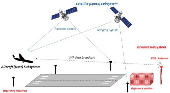
As mentioned above, in view of the stringent civil aviation requirements specified by ICAO [1], augmentations systems were developed for improving performances beyond core constellations performance. In particular, for precision approaches, GBAS (Ground Based Augmentation System) was defined and use the Differential GNSS (DGNSS) technique that significantly improves both the accuracy and the integrity within a local coverage area around the airport. This system is intended to provide an alternative to the already implemented Instrument Landing System (ILS) which suffers from a number of limitations and siting constraints. Then, the term GBAS Landing System (GLS) [12] was assigned to the approach procedure/capability provided by such a system (precision approaches and landing operations).

Today, GBAS installations are standardized to provide precision approaches down to Category I (CAT-I) and are based on GPS and GLONASS using a single frequency (GPS L1 C/A). GBAS CAT II/III service with a single protected signal (GPS L1 C/A) is at an advanced stage of development and standardisation.

It is expected that the evolution of GBAS towards multi-constellation (MC) and multi-frequency (MF) provide better performance and robustness as well as availability of services. In this PhD project and from a European perspective the multi-constellation focus is on GPS/GALILEO.

1.2 Objectives and Contributions

1.2.1 Objectives

In the Civil Aviation domain, research motivations are currently related to the wish to improve airspace capacity, efficiency and safety thanks to the modernization of existing Navigation aids (Navaids), the addition of new infrastructures or addition and modification of user and ground processing. These research motivations will

obviously depend on political motivations. For example, the building of the Galileo constellation in Europe has an impact on European researches and applications about this new element. Consequently motivations will depend on regions where Civil Aviation applications will be applied and developed.That is why, in Europe, research activities within the SESAR project have focused on the use of GPS and Galileo constellations.

As mentioned in the section above, current GBAS is based on GPS and GLONASS constellations and provides precision approach service down to Category I (CAT-I) using a single protected signal (GPS L1 C/A). The evolution of GBAS towards Multi-Constellation (MC) and Multi-Frequency (MF) is expected to provide better performance and robustness as well as availability of services. Several expected improvements [9] are listed below:

 The MC/MF GNSS implementation and particularly the apparition of multiple constellations will provide additional ranging sources thus improving the availability of service (by improving the geometry of the position solution). Furthermore, it will also improve continuity of service that will increase operational robustness and enable advanced applications. Indeed, in some regions ionospheric scintillation can cause loss of service. This issue could be solved with the MC/MF GNSS implementation because with more satellites in view it would be much less likely that scintillation would result in loss of service. So, the availability of additional ranging sources and frequencies will improve the operational robustness.

 With the future implementation of Galileo constellation, MC will provide constellation diversity which limits the dependency from GPS especially in case of a total constellation failure which is a concern of some European institutions and stakeholders. However, from an avionics perspective, greater diversity adds significant complexity to receiver design and thus the associated cost to some stakeholders represents a significant offset to the benefits.

 Future satellites will provide signals for multiple frequencies which allow eliminating errors (or at least mitigating them) caused by the ionospheric threat mitigation during approach and landing operations. Single frequency GBAS L1 CAT III (known as GAST-D) faces demanding constraints linked to requirements for protecting the system against anomalous ionosphere conditions such as equipment & siting requirements, ionosphere threat space, ground and airborne monitoring. Dual-Frequency (DF) processing is expected to overcome at least some of these constraints. [13]

 In addition to DF, new satellites will provide better designed signals [14] (longer codes, higher data rates, message error detection, control methods use of pilot channels, multiplexing) with higher power (much higher with L5 signals) which should provide better accuracy and monitoring performance (noise, multipath, interference rejection). This will lead to better performance of GBAS corrections and also has some impact on particular facility constraints (possibility to have a narrower correlator, a more robust tracking in challenge environment, etc.). [13]

With the introduction of Multi-Frequency, Multi-Constellation SIS (Signal In Space) having different characteristics than GPS L1 C/A SIS, a reconsideration of the current GBAS architecture is required to take the best advantage of the new SIS performance. Indeed, many improvements could be noted by the MF/MC GNSS

such as mitigation of anomalous atmospheric effects, increased availability, stronger robustness to unintentional interference and better accuracy performance due to modernized signal. However, several challenges and key issues must be resolved before the potential benefits may be realized, these include: deriving system level requirements, optimizing the MF processing at ground and aircraft sides, defining VHF Data Broadcast (VDB) transmission and format of the transmitted message from the GBAS VDB unit [4], management of dual constellation at ground and aircraft sides, Galileo fault modes, ground subsystem monitoring and technology, safety, airborne technology, airborne performance and certification, operational impact, standardization, validation and certification authorities involvement etc.

In this PhD project, some of these key issues are investigated to define an optimal solution for this MC/MF GBAS. Therefore, issues concerning the available space for message transmission from the GBAS VHF Data Broadcast (VDB) unit [4] are examined with the possibility of providing corrections at a lower rate than the current 2Hz. This alternative approach is needed because today corrections and their integrity are provided in combined messages broadcast every half second (2Hz) and with the evolution to multiple correction types, based on the different signals and observables for two or more constellations this could not be applicable anymore. Furthermore, if future signals from the modernized constellations are needed to be used or in view of the possible expansion further than two constellations then no additional transmission space would be available.

Also, in order to meet the most stringent requirements of Cat II/III precision approach operations several challenges and key issues must be solved relating to atmospheric modelling. Indeed, nowadays ionospheric effect is considered as dominant compared to troposphere therefore the ionospheric and tropospheric spatial gradients are considered as a combined threat. However, there are a number of arguments for revisiting this topic. Firstly, recent observations, reported at last ICAO NSP meeting [5], showed unexpected atmospheric behavior. These observations have been confirmed by the FAA (Federal Aviation Administration) [15] and Boeing and have shown that significant spatial gradients with no link to ionosphere activity are likely to appear mainly during warm and sunny days. The source could be related to a non-modelled behavior of the troposphere. Even if the range errors induced by this phenomenon are not significant compared to those due to ionospheric gradients, the combination of these “troposphere” gradients with ionospheric gradients could lead to missed detection or false detection of the ground subsystem’s ionospheric monitor, thus impacting integrity and continuity. Secondly, in the advent of DF GBAS, the ionosphere may feasibly be reduced significantly through the ionosphere-free smoothing technique. Under such a scenario, the troposphere threat model may need to be changed and a means for bounding the potential errors derived.

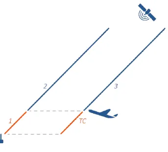
The spatial differential range tropospheric delay can be decomposed into two components: the horizontal component (differential tropospheric delay between aircraft and ground assuming aircraft and ground are at the same altitude) and the vertical component (differential tropospheric delay between aircraft and ground assuming aircraft and ground are not at the same altitude but are at the same latitude and longitude). Both are represented in the following Figure 1 where the differential range delay between paths 2 and 3 (above the aircraft height) define the horizontal component of the differential range tropospheric delay. The vertical

component of the differential range tropospheric delay is represented by the path 1 and is modelled by the standardized vertical Tropospheric Correction (TC) [16]sent to the aircraft.

Figure 1-GBAS Troposphere Delay Paths

Previous work undertaken at Ohio University [5] [6] [7] highlighted the need to consider range horizontal troposphere gradients as a possible source of failure.

That is why, this thesis contains a specific analysis of the tropospheric modelling for both nominal and non-nominal cases and the development of an innovative methodology for bounding these errors.

Therefore this PhD work has initiated the process of assessing the troposphere threat by determining the optimal Dual Constellation (DC)/ Dual Frequency (DF) GBAS processing.

1.2.2 Original Contributions

The main contributions of this thesis are summarized below and detailed all along this report. Several subjects have been published in papers and conferences. They are mentioned in the different sections of this document and the bibliography.

 Development of an optimal processing scheme for meeting the Cat II/III with the MC/MF GBAS (Chapter 4)

 Derivation of the error budget degradation when using lower frequency corrections than the current GBAS message correction rate of 2Hz (4.2 and 4.3).

 Real data analysis for validating the theoretical analysis of this error budget degradation (4.3).

 Development of a worst case horizontal differential range tropospheric ranging delay search methodology using a comprehensive 3D meteorological data model (5.4).

 Determination of horizontal differential tropospheric ranging biases impacting Cat II/III GLS operating aircraft using a comprehensive 3D meteorological data model (5.4).