Multifractal-based texture segmentation using variational procedure

(1)

O

pen

A

rchive

T

OULOUSE

A

rchive

O

uverte (

OATAO

)

OATAO is an open access repository that collects the work of Toulouse researchers and

makes it freely available over the web where possible.

This is an author-deposited version published in :

http://oatao.univ-toulouse.fr/

Eprints ID : 17199

The contribution was presented at IVMSP 2016:

https://signalprocessingsociety.org/blog/2016-ieee-12th-image-video-and-multidimensional-signal-processing-workshop-ivmsp-2016

To cite this version : Frecon, Jordan and Pustelnik, Nelly and Wendt,

Herwig and Condat, Laurent and Abry, Patrice Multifractal-based texture

segmentation using variational procedure. (2016) In: IEEE 12th

Workshop on Image, Video, and Multidimensional Signal Processing

(IVMSP 2016), 11 July 2016 - 12 July 2016 (Bordeaux, France).

Any correspondence concerning this service should be sent to the repository

administrator:

staff-oatao@listes-diff.inp-toulouse.fr

(2)

MULTIFRACTAL-BASED TEXTURE SEGMENTATION USING VARIATIONAL PROCEDURE

Jordan Frecon

1

, Nelly Pustelnik

1

, Herwig Wendt

2

, Laurent Condat

3

, Patrice Abry

1

,

1

Univ Lyon, Ens de Lyon, Univ Lyon 1, CNRS, Laboratoire de Physique, F-69342 Lyon, France. firstname.lastname@ens-lyon.fr 2

IRIT, CNRS UMR 5505, INP-ENSEEIHT, F-31062 Toulouse, France. herwig.wendt@irit.fr 3

Univ Grenoble Alpes, CNRS, GIPSA-Lab, F-38000 Grenoble, France. laurent.condat@gipsa-lab.grenoble-inp.fr

ABSTRACT

The present contribution aims at segmenting a scale-free tex-ture into different regions, characterized by an a priori (un-known) multifractal spectrum. The multifractal properties are quantified using multiscale quantitiesC1,jandC2,jthat quan-tify the evolution along the analysis scales2j_{of the empirical} mean and variance of a nonlinear transform of wavelet co-efficients. The segmentation is performed jointly across all the scales j on the concatenation of both C1,j andC2,j by an efficient vectorial extension of a convex relaxation of the piecewise constant Potts segmentation problem. We provide comparisons with the scalar segmentation of the H¨older expo-nent as well as independent vectorial segmentations overC1 andC2.

Index Terms— Local regularity, multifractal spectrum, segmentation, convex optimization, wavelet leaders

1. INTRODUCTION

Recent contributions in image processing highlighted the need of segmentation techniques for scale-free textures anal-ysis [1, 2, 3]. The possible applications go from texture medical images such as the bone study [4] to art investiga-tions [5, 6].

Scale-free behavior is captured with local regularity, tech-nically measured via the concept of H¨older exponent [7]. First studies based on the estimation of this quantity can be traced back to [8] where local regularity was assumed homogeneous throughout the image (i.e., monofractal). Recent contribu-tions have considered a more realistic model, where the local regularity may be heterogeneous throughout the image (i.e, piecewise monofractal). This further increases the complex-ity of the estimation procedure since it additionnaly amounts in segmenting the image into a priori unknown regions where the local regularity can be considered homogeneous.. Among numerous techniques for image segmentation, some efficient variational approaches have recently been designed relying on the use of the total variation [9, 1, 3, 10]. The good results of these estimation and segmentation techniques (on simulated

Work supported by GdR 720 ISIS under the junior research project GALILEO, ANR AMATIS grant #112432, 2010-2014, and CNRS Imag’in project under grant 2015OPTIMISME.

and real data) thus pave the way for considering more com-plex piecewise scale-free models. This is the subject of the present contribution.

We aim to go further by proposing a segmentation method for piecewise multifractal processes analysis, thus allowing a richer modeling of real-world textures. The multifractal for-malism detailled Section 2 relies on the local estimation of multiscale quantities in place of the local regularity. It is com-bined with a joint vectorial segmentation procedure whose al-gorithmic solution is briefly summarized in Section 3. Esti-mation performance on synthetic results is reported in Sec-tion 4. Comparisons with state-of-the-art methods are also provided.

2. MULTIFRACTAL ANALYSIS

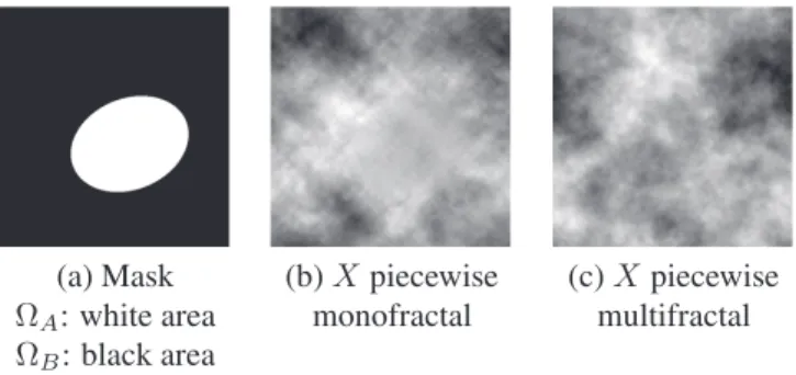
Piecewise mono/multi-fractal. We denoteX = (Xℓ)1≤ℓ≤N the scale-free image to analyze, which hasN pixels. Its local regularity can be quantified by the H¨older exponent [7] de-noted byh = (hℓ)1≤ℓ≤N. While largehℓpoints to a locally smooth portion of the field, lowhℓindicates local high irreg-ularity. Two examples ofX are provided in Figure 1(b)-(c).

On the one hand, in Figure 1(b),X models a piecewise monofractal process having two different values ofhℓ, i.e.

(∀ℓ ∈ ΩA) hℓ= hA, (1) (∀ℓ∈ ΩB) hℓ= hB, (2) withhA < hB andΩ = ΩA∪ ΩB being separable in two distinct areas, i.e.,ΩA∩ ΩB = ∅, according to the mask pre-sented in Figure 1 (a). A smoother behavior is thus observed forℓ ∈ ΩAthan forℓ ∈ ΩB.

On the other hand, in Figure 1 (c),X models a piecewise multifractal process wherehℓ may locally vary both within ΩA and ΩB. Therefore, the multifractal spectrum D(h), which describes local regularity fluctuations, is not reduced to a Dirac (cf. e.g., [7, 11, 12] for details), and

(∀ℓ ∈ ΩA) hℓcan be described byDA(h) (3) (∀ℓ∈ ΩB) hℓcan be described byDB(h). (4) The aim of multifractal analysis is to estimateD(h). For prac-tical purposes, the multifractal spectrum can often be approx-imated as a parabola: D(h) = 2 + (h − c1)2_{/(2c2). Here,}

(3)

(a) Mask (b)X piecewise (c)X piecewise ΩA: white area monofractal multifractal ΩB: black area

Fig. 1. Examples of scale-free textures.

we follow the efficient procedure proposed in [12] based on

wavelet-leadercoefficients [7].

Wavelet-leader coefficients. We denoted(m)_j,k = hX, ψ_j,k(m)i the (L1_{-normalized) 2D discrete wavelet coefficients of}_{X at} location k = 2−j_{ℓ, at scale 2}j _with _{j ∈ {1, . . . , J}, and} wherem stands for the horizontal/vertical/diagonal subband. For a detailed definition of the 2D-DWT, readers are referred to e.g., [13]. The wavelet leader coefficient Lj,k, located around positionℓ = 2j_{k, is defined as the local supremum of} all wavelet coefficients taken within a spatial neighborhood across all finer scales2j′

≤ 2j_{, that is,} Lj,k= sup m=1,2,3, λj′ ,k′⊂Λj,k |d(m)_j′_,k′|, (5) withλj,k= [k2j_{, (k+1)2}j_{), and Λj,k}₌S p∈{−1,0,1}2λj,k+p.

An illustration is provided in Figure 2 whereLj,kis indicated with a black cross and the neighborhoodΛj,kis displayed in red.

H¨older exponent. The H¨older exponent can be obtained by a linear regression of wavelet-leader coefficients as follows:

hk= X

j∈{1,...,J}

wj,klog2Lj,k, (6) where thewj,kmodel regression weights [11].

Multifractal spectrum. The multifractal spectrum can be obtained by multiscale quantitiesC1,j ∈ RN _and_C2,j _{∈ R}N defined as the sample estimates of the first and second cumu-lant oflog2Lj at each given scale2j. It has been shown that C1,j andC2,j are related to the multifractal spectrumD(h) via the coefficientsc1andc2as follows [12]:

EC1,j = c01+ c1ln 2j, (7) EC2,j = c0

2+ c2ln 2j. (8) To evaluate changes in multifractal spectrum, one could nat-urally consider estimatingC1,j andC2,j locally in a neigh-borhood of each pixelℓ, estimate the corresponding local pa-rametersc1andc2, and then perform a vectorial segmentation

Fig. 2. waveleter-leader coefficients. The wavelet leader coefficient (black cross) is defined as the local supremum of all wavelet coefficients taken within a spatial neighborhood across all finer scales (red)

of(c1, c2). However, this relies on the strong assumption that real-world textures follow precisely the scaling behaviors pre-scribed in Eqs. (7) and (8) above. In the present contribution, it has been chosen to relax this requirement and to directly perform a vectorial segmentation over multiscale quantities C1,j andC2,j, possibly smoothed.

3. VECTORIAL SEGMENTATION

We propose to follow segmentation procedure ideas that per-form well for piecewise mono/multi-fractal estimation [2]. The vectorial segmentation procedure is based on a convex relaxation of the piecewise constant Potts segmentation prob-lem [9, 14]. Here we consider the extension to joint vectorial segmentation proposed in [9] for image labelling. In what fol-lows,Y = (Ym)1≤m≤M ∈ RN×M _{can either model}_{h (i.e.,} M = 1), C1 orC2 (i.e., M = J), or their concatenation (C1, C2) (i.e., M = 2J).

Problem formulation. The labeling procedure ofY into Q level sets can be formalized as a minimization problem where Q + 1 binary images Θ = (θq)1≤q≤(Q+1) ∈ RN×Q+1 _are estimated such that

min Θ Q X q=1 (θq−θq+1)⊤ M X m=1 (Ym−vq,m)2_+λ Q X q=1 TV(θq−θq+1) subject to      θ1= 1, θQ+1 = 0, 1 ≥ θ2≥ . . . ≥ θQ≥ 0, (9)

withλ > 0 and where TV denotes the usual total-variation penalization as defined in [15], i.e., for everyθ ∈ RN_,

TV(θ) = N X

ℓ=1

k(Dθ)ℓk2, (10)

(4)

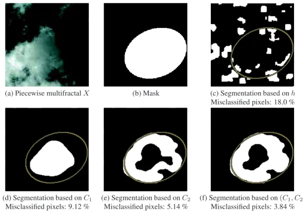
(a) Piecewise multifractalX (b) Mask (c) Segmentation based onh Misclassified pixels: 18.0 %

(d) Segmentation based onC1 (e) Segmentation based onC2 (f) Segmentation based on(C1, C2) Misclassified pixels: 9.12 % Misclassified pixels: 5.14 % Misclassified pixels: 3.84 %

Fig. 3. Illustration of the segmentation results. The piecewise multifractal imageX is presented in (a) and has been generated from the mask (b). The scalar segmentation result obtained fromh is displayed in (c). The vectorial segmentation results based onC1,C2and(C1, C2) are respectively presented in (d), (e) and (f).

difference operator and thus (Dθ)ℓ ∈ R2_{. The choice of} vq,m∈ R will be discussed further.

TheQ resulting labelling areas (Ω1, . . . , ΩQ) are obtained from the binary images(θq− θq+1)1≤q≤Qas follows:

(∀ℓ∈ Ω) θq,ℓ− θq+1,ℓ= (

1, if ℓ ∈ Ωq,

0, otherwise. (11) The first term in (9) is a data fidelity term allowing to impose similar properties within each areaΩq. The second term imposes the regularity for each labelling areaΩq. The smaller isλ the higher is the granularity of Ωq.

Algorithmic solution. In order to efficiently estimateΘ we use the algorithmic strategy proposed in [16] that consists in using a proximal splitting method coupled with an efficient strategy to compute the involved proximal operators. The reader could refer to [9, 16] for details regarding the algo-rithmic strategy for solving (9).

4. EXPERIMENTS

Experimental setting. Performance of the proposed seg-mentation procedure are assessed on synthetic data, numeri-cally produced by inclusion of a 2D MRW patchΩA[17] into

a 2D-MRW backgroundΩB with different multifractal pa-rameters. Patch and background (Figure 3 (b)) have been nor-malized to ensure that the local variance does not depend on the image location. An illustration is provided in Figure 3 (a) where the background parameters(c1, c2) = (0.7, 0.1) and the patch parameters(c1, c2) = (0.4, 0.005).

The wavelet leader coefficients are estimated using a stan-dard2D-DWT with orthonormal tensor product Daubechies mother wavelets with2 vanishing moments.

In our simulation, we have setQ = 2, λ = 1 and J = 3. For every componentm ∈ {1, . . . M }, (vq,m)1≤q≤Qare ini-tially chosen to be equally distributed between the minimum and maximum values ofYm. Then, an alternate minimization of (9) and re-estimation of the(vq,m)1≤q≤Q is performed 5 times.

Scalar vs. vectorial segmentation. The scalar segmentation ofY = h, originally envisaged for the analysis of piecewise monofractal processes [3], is illustrated in Figure 3-(c)). We observe that it yields poor results. Indeed, since the process is multifractal, everyh of the support of D(h) is present in any open interval of the trajectory for finite resolution data. The local estimation ofh is hence not very meaningful. In addition, sinceDAandDBoverlap, the sole featureh can not permit to discriminate betweenΩA andΩB. This limitation

(5)

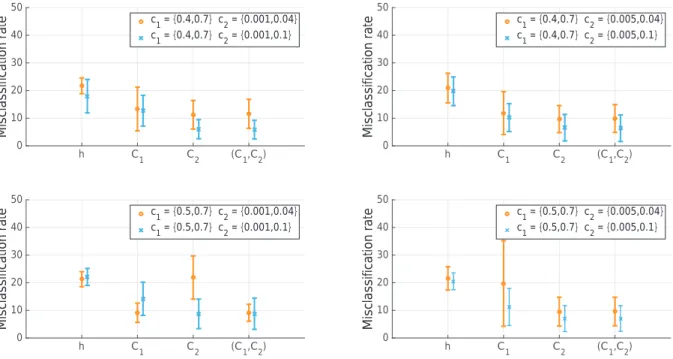
h C 1 C2 (C1,C2) Misclassification rate 0 10 20 30 40 50 c 1 = {0.4,0.7} c2 = {0.001,0.04} c 1 = {0.4,0.7} c2 = {0.001,0.1} h C 1 C2 (C1,C2) Misclassification rate 0 10 20 30 40 50 c 1 = {0.4,0.7} c2 = {0.005,0.04} c 1 = {0.4,0.7} c2 = {0.005,0.1} h C 1 C2 (C1,C2) Misclassification rate 0 10 20 30 40 50 c 1 = {0.5,0.7} c2 = {0.001,0.04} c 1 = {0.5,0.7} c2 = {0.001,0.1} h C 1 C2 (C1,C2) Misclassification rate 0 10 20 30 40 50 c 1 = {0.5,0.7} c2 = {0.005,0.04} c 1 = {0.5,0.7} c2 = {0.005,0.1}

Fig. 4. Segmentation performance. Comparison of the segmentation performance is quantified in terms of mean misclassifi-cation rate depending on the choice of the inputY represented along the x-axis (error bar indicate the standard deviation). Each plot represent two configurations (blue and orange) ofc1andc2onΩAandΩB.

thus shows the need of investigating multiscale quantities re-lated to the multifractal spectrum, namelyC1 andC2. Such a strategy has been previously investigated in [2] with a dif-ferent algorithmic solution involving a difdif-ferent segmentation for each componentm ∈ {1, . . . , M }.

Segmentation performance. For the same patch displayed in Figure 3 (b), we have considered eight configurations re-ported in Figure 4 and defined as follow. The top (resp. bot-tom) plots correspond to a large (resp. small) difference ofc1 betweenΩAandΩB. The left (resp. right) plots model large (resp. small) difference ofc2betweenΩAandΩB. In addi-tion, we have further investigated the impact ofc2: results in orange correspond to two tight multifractal spectrumDAand DB(i.e., smallc2on bothΩAandΩB) whereas the blue one models one tightDA(i.e., smallc2onΩA) and a widespread DB(i.e., largec2onΩB). Estimation performance are quan-tified in terms of misclassified pixels percentage over 20 real-izations for all the different inputsY .

Unsurprisingly, usingY = h always leads to poor seg-mentation performance. In addition, all these experiments reproduce the expected behavior that the larger is the dif-ference ofc1 (resp. c2) betweenΩA andΩB, the better are the segmentation performance associated toY = C1 (resp. Y = C2). However, a closer inspection shows that a larger difference inc1 does not necessarily lead to better segmen-tation results forY = C2 (see the orange line in both left

plots). Overall, we observe that there is always an interest in combining the information of bothC1andC2.

Finally, it is worth noticing that the scalar segmentation ofh is only 2 times faster than the vectorial ones either based onC1,C2or(C1, C2). Experimentally, it takes less than 1 minute per image of sizeN = 29_{× 2}9_.

5. CONCLUSIONS AND PERSPECTIVES

In this work, we have designed an analysis procedure for deal-ing with piecewise multifractal processes. We have shown the need of considering multiscale quantities C1 and C2 rather than the sole H¨older exponent usually considered for piece-wise monofractal processes. An efficient joint vectorial seg-mentation procedure is proposed and yields satisfactory per-formance when applied to(C1, C2).

However, the proposed segmentation procedure rely on the strong assumption that θq,1− θq+1,1 = . . . = θq,M − θq+1,M. Therefore, the performance are very sensitive to the arbitrary choice and order of the level setsvq,m. In order to alleviate this limitation, different regularization terms are under current investigation to provide a more flexible joint vectorial segmentation strategy.

(6)

6. REFERENCES

[1] C. Nafornita, A. Isar, and J. D. B. Nelson, “Semi-local Hurst estimation via generalised lasso and dual-tree complex wavelets,” in Proc. Int. Conf. Image

Pro-cess., Paris, France, Oct. 27-30 2014, pp. 2689–2693. [2] J. Frecon, N. Pustelnik, H. Wendt, and P. Abry,

“Mul-tivariate optimization for multifractal-based texture seg-mentation,” in Proc. Int. Conf. Image Process., Quebec City, Canada, Sept, 27-30 2015.

[3] N. Pustelnik, H. Wendt, P. Abry, and N Dobigeon, “Local regularity, wavelet leaders and total variation based procedures for texture segmentation,,” Tech. Rep., arXiv:1504.05776, 2016.

[4] C.L. Benhamou, S. Poupon, E. Lespessailles, S. Loiseau, R. Jennane, V. Siroux, W. J. Ohley, and L. Pothuaud, “Fractal analysis of radiographic trabecular bone texture and bone mineral density: two complementary parameters related to osteoporotic fractures,” J. Bone Miner. Res., vol. 16, no. 4, pp. 697–704, 2001.

[5] P. Abry, S. Jaffard, and H. Wendt, “When Van Gogh meets Mandelbrot: Multifractal classification of paint-ing’s texture,” Signal Process., vol. 93, no. 3, pp. 554– 572, 2013.

[6] C. R. Johnson, P. Messier, W. A. Sethares, A. G. Klein, C. Brown, P. Klausmeyer, P. Abry, S. Jaffard, H. Wendt, S. G. Roux, N. Pustelnik, N. van Noord, L. van der Maaten, E. Postma, J. Coddington, L. A. Daffner, H. Murata, H. Wilhelm, S. Wod, and M. Messier, “Pur-suing automated classification of historic photographic papers from raking light photomicrographs.,” Journal

of the American Institute for Conservation, vol. 53, no. 3, pp. 159–170, 2014.

[7] S. Jaffard, “Wavelet techniques in multifractal analy-sis,” in Fractal Geometry and Applications: A Jubilee

of Benoˆıt Mandelbrot, M. Lapidus and M. van Franken-huijsen Eds., Proceedings of Symposia in Pure Math-ematics, M. Lapidus and M. van Frankenhuijsen, Eds. 2004, vol. 72, pp. 91–152, AMS.

[8] S. G. Roux, A. Arneodo, and N. Decoster, “A wavelet-based method for multifractal image analysis. III. Ap-plications to high-resolution satellite images of cloud structure,” Eur. Phys. J. B, vol. 15, no. 4, pp. 765–786, 2000.

[9] A. Chambolle, D. Cremers, and T. Pock, “A convex approach to minimal partitions,” SIAM J. Imaging Sci., vol. 5, no. 4, pp. 1113–1158, 2012.

[10] J.D.B. Nelson, C. Nafornta, and A. Isar, “Semi-local scaling exponent estimation with box-penalty con-straints and total-variation regularization,” IEEE Trans.

Image Process., vol. 25, no. 6, pp. 3167–3181, Apr. 2016.

[11] H. Wendt, P. Abry, and S. Jaffard, “Bootstrap for empir-ical multifractal analysis,” IEEE Signal Process. Mag., vol. 24, no. 4, pp. 38–48, Jul. 2007.

[12] H. Wendt, S.G. Roux, P. Abry, and S. Jaffard, “Wavelet leaders and bootstrap for multifractal analysis of im-ages,” Signal Proces., vol. 89, pp. 1100–1114, 2009. [13] S. Mallat, A wavelet tour of signal processing,

Aca-demic Press, San Diego, USA, 1997.

[14] M. Storath and A. Weinmann, “Fast partitioning of vector-valued images,” SIAM J. Imaging Sci., vol. 7, no. 3, pp. 1826–1852, 2014.

[15] A. Chambolle, “An algorithm for total variation mini-mization and applications,” J. Math. Imag. Vis., vol. 20, no. 1-2, pp. 89–97, Jan. 2004.

[16] L. Condat and N. Pustelnik, “Segmentation d’image par optimisation proximale,” in Proc. GRETSI, Lyon, France, September 8-11, 2015, in French.

[17] Raoul Robert, Vincent Vargas, et al., “Gaussian mul-tiplicative chaos revisited,” The Annals of Probability, vol. 38, no. 2, pp. 605–631, 2010.