The influence of shrub expansion on albedo and the winter radiation budget in the Canadian Low Arctic

(1)

The influence of shrub expansion on albedo and the

winter radiation budget in the Canadian Low Arctic

Thèse

Maria Belke Brea

Doctorat en sciences géographiques

Philosophiæ doctor (Ph. D.)

(2)

The influence of shrub expansion on albedo and the

winter radiation budget in the Canadian Low

Arctic

Thèse – Doctorat en sciences géographiques

Maria Belke-Brea

Sous la direction de:

Florent Dominé, directeur de recherche

Ghislain Picard, codirecteur de recherche

Stéphane Boudreau, codirecteur de recherche

(3)

Résumé

Au cours des dernières décennies, le réchauffement climatique a entrainé une arbustation accélérée des écosystèmes arctiques. En modifiant l’albédo, les arbustes influencent la température de l’atmosphère, du manteau neigeux et du pergélisol, ce qui pourrait accélérer la fonte ou le dégel de ces deux derniers et initier de fortes boucles de rétroaction positive qui accentueraient les effets des changements climatiques. L’une des conséquences principales de cette arbustation est la réduction de l’albédo de la neige par les branches qui dépassent du manteau neigeux et en assombrissent la surface. De plus, des interactions complexes entre neige et arbustes d’une part modulent la remobilisation et le transport de la neige par le vent et d’autre part accélèrent la fonte durant les redoux. Ainsi, la présence d’arbustes au sein du manteau neigeux peut affecter les propriétés physiques et optiques de la neige, altérant encore davantage l’albédo de la surface affectée. Enfin, les branches ensevelies dans la neige peuvent également influencer le budget radiatif en absorbant les rayons lumineux car ceux-ci pénètrent généralement à plus de 10 cm de profondeur dans le manteau neigeux. Pour étudier et quantifier les interactions entre la neige, les arbustes et la lumière, nous avons récolté un jeu de données unique qui compare des manteaux neigeux avec et sans arbustes. Pour tous les sites échantillonnés, nous avons mesuré l’albédo spectral in situ et les profils de propriétés physiques de la neige ainsi que d’irradiance. Nous avons récolté ces données dans le bas Arctique, à Umiujaq, Nord du Québec, Canada (56° N, 76° W), au cours de plusieurs campagnes de terrain d’automne et d’hiver. En nous basant sur les données obtenues ainsi que des données de taille et de distribution verticale de branches d’arbustes, nous avons développé et validé une paramétrisation simple mais efficace permettant de modéliser l’albédo de surfaces hétérogènes composées de neige et d’arbustes. Cette nouvelle paramétrisation nous a permis de modéliser l’albédo avec une erreur inférieure à 3 %. Elle peut être utilisée de manière prédictive et est facile à intégrer aux modèles de système terre.

(4)

L’albédo ainsi modélisé nous a permis d’élucider des processus importants des interactions entre la neige, les arbustes et la lumière. Nous avons trouvé que la réduction de l’albédo par les branches qui dépassent du manteau neigeux dépend de la longueur d’ondes considérée. Tôt durant la saison nivale, les branches diminuent l’albedo de 55 % à 500 nm et 18 % à 1000 nm. En revanche, l’effet des branches sur les propriétés physiques de la neige n’étaient pas suffisamment importants pour affecter l’albédo, sauf lors d’évènements climatiques extrêmes comme les blizzards ou les épisodes de chaleur. Nos résultats suggèrent que l’impact direct de l’assombrissement par les branches est largement supérieur aux effets indirects causés par les changements des propriétés physiques de la neige. Cependant, ces derniers pourraient gagner en importance si les évènements climatiques extrêmes devenaient plus fréquents au fur et à mesure que le réchauffement de l’Arctique s’intensifie. Finalement, nous montrons que l’impact des branches ensevelies sous la neige se traduit surtout par une augmentation de la fonte durant les épisodes de chaleur ainsi que par une intensification des processus métamorphiques tôt dans la saison. Cependant ces impacts étaient extrêmement localisés et restreints à l’environnement très proche des branches. Pour cette raison, il a été difficile de quantifier l’impact des branches ensevelies sur le budget radiatif terrestre, d’autant plus que les concentrations de carbone suie élevées (185 ng g-1_{) dans le manteau neigeux d’Umiujaq ont accentué l’incertitude}

quant à l’effet relatif de ces deux processus sur l’albédo.

Finalement, comme notre paramétrisation pour modéliser l’albédo a été développée sur la base de données provenant d’un seul site, nous croyons qu’il serait nécessaire de la tester de manière plus générale, avec des données provenant d’autres endroits. De cette manière, elle pourrait ensuite être intégrée aux modèles de surface continentale, ce qui permettrait d’inclure un effet réaliste de l’arbustation actuelle et future de l’Arctique sur les scénarios climatiques locaux et globaux.

(5)

Abstract

Arctic warming is causing an expansion of deciduous shrubs in the Arctic tundra biome. By modifying albedo, shrubs affect the temperature of the atmosphere, snowpack and permafrost, potentially increasing permafrost thawing and snow melting, and forming a powerful feedback to global warming. The most prominent impact of shrubs is a reduction of surface albedo when dark branches protrude above the bright snow surface. Additionally, complex snow-shrub interactions modify snow redistribution during windy conditions and increase snowmelt rates during warm spells. Thus, snow over shrub-covered tundra may have different physical and optical properties, leading to further modification of surface albedo. Finally, shrub branches buried in snow may still have an impact on the radiation budget because they can absorb light rays which generally penetrate deeper than 10 cm into the snowpack. To study and quantify the snow-shrub-light interactions, we collected a unique dataset comparing snowpacks with and without shrubs. For every site sampled, we measured in situ spectral albedo (400–1080 nm) and recorded snow physical properties and irradiance profiles. These data were acquired in a low Arctic site near Umiujaq, Northern Quebec, Canada (56° N, 76° W), during several field campaigns in autumn and winter. Based on these field data and a dataset of branch sizes and vertical distribution, a simple yet accurate parameterization for modeling albedo of mixed snow-shrub surfaces was developed and validated. This new parameterization had an accuracy of 3 %, can be used in a predictive way, and is easy to implement in earth system models.

We uncovered important insights on snow-shrub-light interactions. Surface darkening by protruding branches was wavelength-dependent, and decreased albedo early in the snow season by 55 % at 500 nm and 18 % at 1000 nm. Changes in snow physical properties that were significant enough to impact albedo only occurred in conjunction with extreme weather events like after blizzards or during warm spells. Thus, the direct impact of darkening from shrubs likely dominates over the indirect impact from changes in snow

(6)

physical properties, however the latter may gain in importance if extreme weather events become more frequent as Arctic warming progresses. The impact of buried branches was very localized, increasing snow melting during warm spells and enhancing snow metamorphic processes early in the season in the direct vicinity of branches. However, quantifying the impact of buried branches on the radiation budget was challenging due to their highly localized effect and because of high black carbon concentrations in the snowpack at our study site, which reached 185 ng g-1.

We suggest that future research test the parameterization developed here more broadly, as this study was based on data from just one study site. The parametrization can then be implemented into land surface models, allowing for reliable estimates of the effect of current and projected Arctic shrubification on global and regional warming.

(7)

Liste of Tables

2.1 Snow depth in cm at the lichen site S0, small shrub site S1 (~36 cm), the medium shrub site S2 (~80 cm) and the tall shrub site S3 (~120 cm). Snow depth was measured with a snowprobe……….. 43 3.1 Snow depth in cFitted coefficients for the global and location-specific allometric equations

(Eq. (3.2)) and their standard errors………... 77 4.1 Average snow height and shrub height in Umiujaq for the three shrub-free snowpacks and

the four snowpacks with shrubs………. 102 4.2 Fit between measured and calculated extinction coefficient curves (ke(λ)) for measurements

in shrub-free snowpacks. Calculated ke(λ) was computed either with black carbon (BC), BC

and mineral dust, or mineral dust only. The fit between measured and calculated ke(λ) was

analyzed with the coefficient of determination (R2_{), the error is indicated with the root mean}

(10)

Liste of Figures

0.1 Overview of different spectral albedo plots including the high albedo of pure and small-grained snow and the low albedo of dirty and large-small-grained snow which show the range of albedo values for snow covered surfaces. All snow albedo plots were calculated using the radiative transfer model TARTES (Libois et al. 2013). Also shown is the albedo of Betula nana shrubs as measured in Siberia by Juszak et al. (2014). Shrub albedo is considerably

lower than snow albedo, particularly in the visible range………... 2

0.2 Contrast of a bright snow surface and a mixed snow-shrub surface darkened by protruding

branches in Umiujaq……… 4

1.1 Schema of the Earth’s radiative fluxes. Solar radiation is shown as yellow arrows and terrestrial radiation as red arrows Image source: http://science-edu.larc.nasa.gov/energy_budget/ quoting Loeb et al. 2009 and Trenberth et al. 2009………. 6 1.2 Global temperature anomalies (upper graph) measured from 1880 to present and increase in

the atmospheric CO2 concentration (lower graph) measured at the Mauna Loa Observatory, Hawaii. Atmospheric CO2 concentrations increased steeply since the onset of measurements in 1960 and global temperatures have been rising since the 1970s. Data sets to create the image were taken from NASA, NOAA and the UCSD institution of oceanography………….. 11 1.3 Global temperature change over the time period 1884 to 2019, which highlights the amplified

Arctic warming. Temperature differences are shown compared to a baseline average from

1951 to 1980……… 12

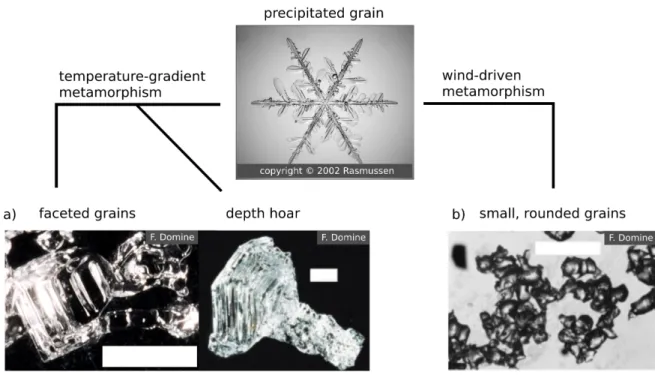
1.4 Shape of snow grains after metamorphism. White scale bars on photographs are 1 mm. a) faceted grains and depth hoar created by temperature-gradient metamorphism. b) small,

rounded grains created by wind-driven metamorphism……….. 17

1.5 Sketch of light scattering at a single grain (left) and of scattering and absorption within a snowpack (right). The yellow arrow on the left shows one possible path light takes within the area of scattering for a single grain. The yellow arrows on the right side show possible paths that incoming light can take when penetrating the snowpack before re-emerging at the

surface……….. 19

1.6 Sketch of different scattering behaviors. Snow has a strong forward scattering………. 20 1.7 a) measured absorption coefficient for ice (from Picard et al. 2016). b) typical albedo curve

for a pure snow surface (black), a pure snow surface with large grains (red) and a snow surface with impurities (blue) as calculated with snow radiative transfer model TARTES…… 20 1.8 Modified sketch from Warren (1982) of the impact of the Solar Zenith Angle (SZA). The

deeper penetration at low SZA increases the pathlength in the snow, therefore increasing the

probability of absorption and decreasing albedo………. 23

2.1 Location of study sites and automatic weather station in the Tasiapik Valley near Umiujaq in Northern Quebec, Canada. Map source: Natural Resources Canada

(11)

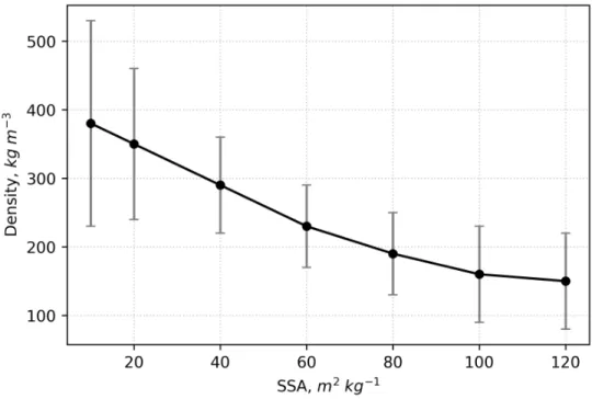
2.2 Empirical correlation of snow density and SSA for surface snow based on 5 years of snow

measurements near Umiujaq……… 40

2.3 Four shrub albedo spectra used as αveg input parameter for simulations with the LME (Eq.

(2.1)). The spectra include (1) the average of five albedo spectra measured in late summer 2015 near Umiujaq (αveg_umi) over Betula glandulosa shrubs, (2) two measurements conducted

by Juszak et al. (2014) with a contact probe in Siberia for young (αveg_y) and old (αveg_o)

branches of Betula nana shrubs and (3) one average spectra of Juszak’s young and old branch

spectra (αveg_y+o)……… 42

2.4 Comparison of spectral albedo measured in Umiujaq on 8 Nov. (a), 15 Nov. (b) and 22 Nov. (c) 2015 at four different sites (S0 - S3). S0 is a lichen site with a pure snow surface, S1-S3 are shrub sites with shrubs of different heights: ~36 cm (S1), ~ 80 cm (S2) and ~ 120 cm (S3) 44 2.5 Photographs taken during the autumn campaign illustrating snow-wind-melting interactions.

(a) increased melting in shrubs during the warm spell on 6 and 7 Nov. (b)……… 45 2.6 SSA profiles measured for the upper 10 cm of the snowpack near Umiujaq on 8 Nov. (a), 15

Nov. (b) and 22 Nov. (c) 2015 at the four different study sites S0 to S3. Different meteorological conditions, preceded the three days: before 8 Nov. temperatures were close to 0 °C and we observed melting. Before 15 Nov. wind speeds were extremely high (16 m s ¹)⁻ and before 22 Nov. snow precipitated under cold and calm conditions. Instrument problems

prevented SSA acquisition at S1 on 8 Nov……….. 46

2.7 Determination of the scaling factors used to correct artifacts in measured albedo. (a) Spectral snow albedo observed at the lichen site S0 on 22 Nov. αsn_obs (black) is the measured snow

albedo. αsn_TARTES (red) is the theoretical snow albedo computed with TARTES from the SSA

profiles. αsn_obs, corrected (blue) is the measured spectrum after correction with A=0.958. (b)

Deduced scaling factors for all 13 snow albedo measurements taken at S0 during the autumn

campaign 2015 in Umiujaq……….. 47

2.8 Illustrating the fit between observed albedo at shrub sites S2 and S3 (αmix_obs, corrected, black)

and simulations with the LME (Eq. (2.1)). Simulations in red used the best-fitting αveg

spectra, all other colors (green, blue and yellow) are simulations with alternative αveg spectra.

αveg_o and αveg_y are old and young branch reflectivity (Juszack et al. 2014), αveg_y+o is the

average spectra of old and young branches and αveg_Umi is the average of five albedo spectra

measured near Umiujaq. All simulations used snow albedo computed with TARTES

(αsn_TARTES)..………... 48

2.9 Average residuals (solid line) and their standard deviation (dashed line and shaded area) per wavelength for LME simulations conducted with a snow albedo parameter computed with TARTES (αsn_TARTES, red) and a snow albedo parameter derived from snow albedo

measurements at S0 (αsn_obs, blue). ……….. 49

2.10 Spectral incoming radiation for 8 Nov. and 2 Dec. at 17:00 UTC as calculated with SBDART for overcast conditions (top) and spectra of absorbed radiation (middle and bottom) for the lichen site S0 (blue), medium shrub site S2 (green) and tall shrub site S3 (red)………. 51 3.1 Map of the study area around Umiujaq with the albedo, height and SSA measurement sites

marked with a black box and shrub harvesting locations along the coast marked with blue dots and those in the Tasiapik Valley with red diamonds. A white cross marks the position of

the Automatic Weather Station (AWS)……… 66

3.2 Photograph taken during shrub sampling in January 2016. Snow had to be carefully removed to cut branches within each of the 10 cm strata, which are marked by the horizontal plastic

(12)

3.3 The performance of several exposed-vegetation functions is evaluated against the empirical correlation of shrub fraction covered by snow (Hsnow/Hveg) and exposed-vegetation factor fexp.

(a) Empirical correlation determined from stratified samples. No difference is detectable between summer samples (blue crosses) and winter samples (red crosses). (b) Performance of Eq. (3.5) with a shape factor d set to 1 (orange), to 2 (dark-green) or a shape factor of 0.57 determined with a least-square approach (brown). Neither approach could accurately reproduce the empirical data (black crosses). (c) A good fit with the empirical data was achieved by using two linear regressions, one for the lower 75 % of shrubs (black) and a second one for the upper 25 % of shrubs (green)

………. 74

3.4 The performance of several exposed-vegetation functions is evaluated against the empirical correlation of shrub fraction covered by snow (Hsnow/Hveg) and exposed-vegetation…………... 75

3.5 Correlation of adjusted weighting factors (χadj) and calculated weighting factors (χcalc). The

former were taken from Belke-Brea et al. (2019) and are considered reference values. (a) χcalc-values were calculated with Eq. (3.5), the commonly used exposed-vegetation function,

with a shape factor d set to 1 (orange), 2 (dark-green) or 0.57 (brown). (b) χcalc-values were

calculated with Eq. (3.8) and Eq. (3.9) and either the coast allometry (blue), the valley allometry (red) or the global allometry (gray). The 1:1 line had been drawn as a visual aid……….

78 3.6 Example highlighting model sensitivity to the choice of exposed-vegetation function and

allometric equation. Measured albedo, taken on 22 Nov. in the valley near Umiujaq, is shown together with (a) two spectra simulated with different exposed-vegetation functions and (b) three spectra simulated with different allometric equations. All simulated spectra in (b) were calculated using the twofold approach (shown in Eq. (3.8) and (3.9)). The best fit between measured and modeled data was achieved by using the twofold approach together with global

allometry (green curve)……… 79

3.7 Average residuals of 31 measured albedo spectra and the corresponding simulated spectra, the latter calculated either with valley allometry (red), global allometry (grey) or the coast allometry (blue). The average residuals show that albedo was underestimated when calculated with coast allometry, slightly overestimated when calculated with global allometry and more significantly overestimated when calculated with valley allometry……… 81 4.1 Comparison of the spectral absorption of BC (red) and the spectral absorption of branches

(green). Absorption of branches is illustrated by co-albedo measurements (Juszak et al. 2014). Branch absorption is strongly wavelength dependent and decreases sharply for

wavelengths >680 nm……….. 98

4.2 Map of the study area in the Tasiapik Valley near the village Umiujaq. The blue rectangle marks the area where SOLEXS profiles were measured in shrub-free snowpacks. The red dots mark where SOLEXS profiles were measured in snowpacks with shrubs. A white cross marks the position of the Automatic Weather Station (AWS) and the site where waste was burned is marked with a red star……….. 101 4.3 Overview of how the absorption coefficient (ke_meas(λ)) is determined from optically

homogeneous layers in irradiance profiles. (a) Irradiance as a function of depth for selected wavelengths. The blue shaded area highlights an optically homogeneous zone where the recorded signal is linear on logarithmic scale. The red shaded area was discarded due to potential influence of direct light. ke_meas(λ) is the slope of irradiance vs. depth in the optically

homogeneous zone obtained via linear regression (black lines). (b) ke_meas(λ) determined for

each wavelength in the measured spectrum (350–900 nm) before (blue curve) and after smoothing (black curve). The figure layout was adapted from Tuzet et al. (2019) and modified with data from Umiujaq. The presented data was measured in Umiujaq on 22 November 2015……… 110

(13)

4.4 Example for measured and calculated absorption coefficient ke for a snowpack without

shrubs. Measured ke was determined from SOLEXS measurements taken on 8 Nov. (ZOI1).

Calculated ke was computed with either (a) black carbon (BC) or (b) mineral dust as impurity

type in the snowpack. The concentration of dust or BC was determined with an iterative approach, where calculated ke was fitted to the measured ke. This example shows how

assuming BC as impurity type returns significantly better fits……… 112 4.5

Measured log-irradiance profiles (black curves) and MCML simulations (red and blue curves) for snowpacks without shrubs at 400 nm. Simulated profiles were computed assuming black carbon (BC) as impurity type. Log-irradiance profiles were measured on (a) 8 Nov., (b) 22 Nov. and (c) 28 Nov. Gray shaded areas highlight transition zones, where simulated and measured profiles were not expected to fit. Blue shaded areas highlight non-transition zones were the fit between simulated and measured profiles allowed the

determination of impurity concentrations………... 116

4.6 Log-irradiance profiles and MCML simulations at 400 nm for measurements taken on (a) 9 Nov., (b) 3 Nov., (c) 23 Nov., and (d) 14 Nov. in snowpacks with shrubs. Yellow shaded areas highlight layers where measured log-irradiance profiles and MCML simulations fitted well. Green shaded areas highlight layers where log-irradiance and MCML simulations fit less well and branches were visible in the snowpit photographs……… 117 4.7 Measured and calculated ke for (a) ZOIs in shrub-free snowpacks and (b) IMP and BRAN

layers identified in shrub snowpacks (see also Figure 4.6). Gray areas highlight the spectral range where calculated ke was fitted to measured ke. Deviations at wavelengths >680 nm are

interpreted as influence of buried branches………. 120 4.8 Photographs showing cursory observations of localized snow melting around branches (a, b,

c) and the formation of depth hoar pockets around buried branches (d, e). Photographss were taken during the measuring campaign from 29 Oct. to 6 Dec. 2015. In (d) the contrast of the photograph was increased to make the depth hoar pockets more visible……….. 123 A1 Spectral shrub albedo measured during the late summer campaign 2015 for shrubs growing

on lichen (2 measurements), moss (2 measurements) or soil covered by fallen leaves (litter, 1 measurement)………... 146 B1 Correlation of adjusted weighting factor (χadj) and calculated weighting factor (χcalc). The

former was taken from the modeling results of Chapter 1 (Belke-Brea et al. 2019). Vertical error bars indicate the χcalc errors calculated from the error propagation shown in the

Appendix B2……… 147 C1 Comparison of wind speed distributions on the coast and in the valley for the year 2013……. 149 D1 SOLEXS irradiance profiles and SnowMCML simulations at 400 nm (a) and 500 nm (b) for

8 Nov. SnowMCML simulations were computed either with impurity type set to mineral dust (red plots) or BC (black plots). Using BC returns a good fit-quality independent of wavelength, while the fit with dust varies from 400 to 500 nm……….. 150

(14)

List of Acronyms

The acronyms used in this PhD thesis are listed below.

Acronym Meaning

BAI Branch Area Index

BC Black Carbon

DF Degree of Freedom

DUFISSS DUal Frequency Integrating Sphere for Snow SSA measurement

IPCC Intergovernmental Panel on Climate Change

LAI Leaf Area Index

LAP Light Absorbing Particles

LME Linear Mixing Equation

LSM Land Surface Model

MAE Mass Absorption Efficiency

NLS Nonlinear Least-Square regression

RMSE Root Mean Square Error

SBDART Santa Barbara DISORT Atmospheric Radiative Transfer

Snow MCML Monte Carlo modeling of light transport in multi-layered tissues,

for snow

SOLEXS SOLar EXtinction in Snow

SSA Specific Surface Area

SZA Solar Zenith Angle

TARTES Two-Stream Analytical Radiative TransfEr in Snow

ZOI Zone Of Interest to determine extinction coefficients from SOLEXS

(15)

List of Notations

The notations used in this PhD thesis are listed below together with a description. Notations Description

Γsnow-free (snow-free) vegetation fraction used in Liston and Hiemstra (2011)

αmix_obs Measured mixed surface albedo

αmix_obs,corr Measured mixed surface albedo corrected with scaling factor A

αmix_calc Mixed surface albedo calculated with the LME

αsnow Snow albedo parameter in the LME

αsn_obs Measured snow albedo at shrub-free sites

αsn_obs, corr Measured snow albedo at shrub-free sites corrected with scaling factor

A

αsn_TARTES Snow albedo calculated with TARTES using SSA from shrub-free sites

αveg Shrub albedo parameter in the LME

αveg_y, αveg_o,

αveg_y+o

Shrub albedo measured by Juszak et al. (2014) for young branches (αveg_y), old branches (αveg_o) and an average of young and old branches

(αveg_y+o)

χ Weighting factor in the LME

χadj Weighting factor deduced with a least-square approach using measured

albedo

χcalc Weighting factor calculated with allometric approach

ωrod The albedo of the measuring rod in SOLEXS

A Scaling factor, used to correct measured spectral albedo

BAIexposed Branch Area Index of branches protruding above the snow

BAItotal Total Branch Area Index before snow burial

(16)

DFglob, DFloc Degree of freedom for the local (loc) and global (glob) regression used

to establish the BAI–Hveg allometric equation

Esnow, ELAP, Erod,

Eshrub

Material-specific extinction of snow, impurities, the measuring rod and shrubs

F F-ratio calculated with an F-test to compare the quality of fit between

the local model and the global model, see also Eq. (3.3)

Hveg Shrub height, cm

Hsnow Snow height, cm

Ilog Log-irradiance profiles measured with SOLEXS

SSEglob, SSEloc Error sum-of-square for the local (loc) and global (glob) regression

used to establish the BAI–Hveg allometric equation

a, b Fitted coefficients in allometric equations

d Shape factor in exposed-vegetation function

dopt Optical snow grain diameter

k Backscattering factor

ke_calc Extinction coefficient, calculated as a function of snow physical

properties and impurities

ke_meas Extinction coefficient, determined with linear regression from SOLEXS

measurments

(17)

I dedicate this thesis to Gloria Brea Morales. I whish I could share this work with you.

(18)

Snowflakes are one of nature's most fragile things, but just look what they can do when they stick together. Vista M. Kelly

(19)

Acknowledgements

Moving to another country to start a PhD thesis is, quite frankly, a crazy endeavor. There is a new language to be learned, a new culture to be discovered, new ties of friendship to be formed and old ones to be kept alive over a long distance. And then there is the science itself. I could not have survived all of this without a great group of people around me! The first thank you goes to my supervisor, Florent Dominé. You created the conditions for this project to happen, you supported my work financially and you guided me through the obstacles I encountered during my thesis. I also want to give you here the award as the cook of the best ‘northernmost’ tartiflette and ‘northernmost’ apple pie. Next, I want to thank my co-supervisors, Ghislain Picard and Stéphane Boudreau. Ghislain, you were an invaluable adviser and your input on snow optics always improved my work – thank you for that. Stéphane, you helped me out a lot with data on Arctic shrubs, your specialized knowledge on the flora of the Arctic tundra, and last but not least, with much encouraging words. The field work was an essential part of this thesis, and I want to thank all the people who contributed to make this extraordinary arctic experience possible. I am very grateful to the Centre d’Études Nordiques (CEN) for providing and maintaining the Umiujaq research station. The communities of Umiujaq and Pond Inlet were amazing hosts, and they helped me out of several tight spots during the field work. A special thank you goes to Mathieu, you were a great field partner and friend in numerous arctic adventures! You always waited patiently with me for good lighting conditions to measure albedo, no matter how cold it was. Thank you also to Laurent Arnaud, for your advice and for your logistical skills. Finally, I want to thank my family and friends. Most of all, Frédéric LeTourneux, you were always by my side, with comfort food, a big hug and an endless stream of encouraging words – thank you so much for your support! I also want to thank the infamous group of Downtown Partyeurs, in who’s company I could recharge my batteries, and the group at the

(20)

Cabane à Jack – you made the last weeks of writing so much easier. My last but very big thank you goes to Germany to my family and my old friends: thank you for your text messages, your visits and for just being there!

(21)

Avant-propos

This document is a synthesis of my scientific work which has been published, or is in preparation to be published, as scientific articles. The articles are integrated in chapters 2, 3 and 4, justifying the format « thèse – article » of this thesis. Each article chapter was extended by a preamble to make the understanding of the manuscript easier. Writing a thesis in the format « thèse – article » creates some redundancy concerning the description of the study sites, the applied methodologies and the mathematical equations. On the other hand, the chosen format allows that every chapter is read independantly.

The scientific article in Chapter 2 has been published in the peer-reviewed Journal of

Climate on 15 January 2020 under the open access licence (Belke-Brea et al. 2020). I am

first author of this article, was responsable for the field work and the analysis of the data. The co-authors of the article are F. Domine, M. Barrere, G. Picard, L. Arnaud.

The scientific article in Chapter 3 has been accepted by the peer-reviewed Journal of

Hydrometeorologie on 10 August 2020. I am first author of this arcticle and I was

responsible for most of the field work and the developement of the new method presented in the article. The co-authors of the article are F. Domine, S. Boudreau, G. Picard, M. Barrere, L. Arnaud and M. Paradis.

The manuscript in Chapter 4 is in preparation to be submitted to the peer-reviewed journal

Biogeosciences. I am the first author of this mansucript and I was responsible for the field

work as well as the analysis of the field and model data. Model simulations in this article were performed by Ghislain Picard. The co-authors of the manuscript are F. Domine, G. Picard and L. Arnaud.

(22)

Introduction

Snow surfaces – the cooling element in the Earth’s climate system

Snow is a ubiquitous feature of the Northern Hemisphere and may cover up to 49 % of the land surface at its maximal extent in January (Lemke et al. 2007, Déry and Brown 2007). Snow extent is largest at high northern latitudes, where snow covers the ground for most of the year (7–10 months of the year; Callaghan et al. 2012, Barry and Hall-McKim, 2014). Initial research on snow was mainly conducted at lower latitudes because of its importance for water management, for the outdoor industry (e.g. ski) and for detailed avalanche forecasting. However, since 1990, the observed increase in atmospheric CO2 which is

resulting in global warming has increasingly lead researchers to investigate the fundamental role played by snow on the global climate. A question of interest is how changes in snow cover, particularly in the Arctic where snow cover has the largest extent, may positively feedback on global warming.

The importance of snow to the climate system is mainly due to its high reflectivity (albedo) of solar radiation (Figure 0.1). Snow-covered areas increase the planetary albedo, so that a large portion of solar radiation is reflected into space rather than being absorbed by the Earth’s surface. Large expanses of snow-covered areas therefore have an overall cooling effect on the planet. However, rising temperatures due to global warming reduce the extent and duration of the global snow cover, which in turn reduces the cooling effect of snow, and amplifies global warming (Derksen and Brown 2012). As temperatures continue to increase, snow cover decreases further, establishing a powerful positive feedback loop called the snow-albedo feedback.

(23)

The snow-albedo feedback is only partly caused by the loss of snow cover: an equally important role may be attributed to the natural variation of snow albedo (Fernandes et al. 2009, Picard et al. 2012). These variations range between 0.6 and 0.85 in the broadband (350–1000 nm) and depend on snow physical properties such as snow density as well as size and shape of snow grains. Snow grain size is a particularly important determinant of snow albedo, because the larger the grains the higher the probability for light to be absorbed (Figure 0.1) (O’brian and Munis 1975, Warren 1982). The reason for the natural variation of snow albedo is that grain size in the snowpacks changes over time, a process called snow metamorphism (Sommerfeld and LaChapelle 1970, Grenfell and Maykut 1977). Snow metamorphism is driven by meteorological parameters, like wind and temperature, and can have opposite effects on snow grain size. For example, in the Arctic strong winds roll snow grains over the ground abrading them and thus creating layers of small rounded grains (Schmidt, 1984, Domine et al. 2007). In contrast, when temperatures are around 0°C, melt-freezing events can produce snow layers composed of melt-freeze Figure 0.1 Overview of different spectral albedo plots, including the high albedo of pure and small-grained snow and the lower albedo of dirty and large-grained snow. Dirty snow is mixed with 100 ng g-1_{of black}

carbon (BC). This graph shows the range of albedo values for snow covered surfaces. All snow albedo plots were calculated using the radiative transfer model TARTES (Libois et al. 2013). Also shown is the albedo of Betula nana shrubs as measured in Siberia by Juszak et al. (2014). Shrub albedo is considerably lower than snow albedo, particularly in the visible range.

(24)

crystals which have particularly large grain sizes. Because light absorption depends on grain size, snow albedo of wind-drifted small grains is high compared to albedo of a melt-freeze layer with large grains (Figure 0.1). As climate warms air temperatures increase in the Arctic, and snow precipitation, wind patterns and snow melt events change which will impact Arctic snow metamorphism processes and affect snow albedo values.

Another factor that further amplifies the snow-albedo feedback is the warming-induced transition from herb, moss and lichen tundra to shrub tundra which has been observed in the Arctic in the last decades (Tape et al. 2006, Ropars and Boudreau 2012). Erect shrubs can impact winter surface albedo by several processes. The most obvious one results from branches which have low albedo (Figure 0.1) and that protrude above the snow causing a darkening of the formerly bright snow surface (Figure 0.2). In addition, branches that are buried in the snowpack also absorb incoming light and reduce albedo because snow is a translucent medium into which light penetrates up to tens of centimeters (Warren 1982, France et al. 2011, Picard et al. 2016, Tuzet et al. 2019). Finally, complex snow-shrub interactions can alter snow metamorphism and snow grain size, which ultimately changes snow albedo. To calculate the radiative effect of shrub expansion at specific sites or on a pan-Arctic scale, simple linear mixing equations (LME) were used in previous studies (Sturm et al. 2005, Liston and Hiemstra 2011, Ménard et al. 2014). With these LMEs, the albedo of mixed snow-shrub surfaces is calculated as a function of snow and shrub albedo and a factor that weights snow and shrub albedo with respect to the surface they each cover. However, it remains unclear whether or not this simplified linear-mixing approach is suitable as a parameterization of mixed surface albedo because there are few broadband and no spectral albedo in situ measurements against which the model could be validated. Current LMEs neglect the effect of buried branches and of snow-shrub interactions, which may introduce significant inaccuracies to the LME calculations. Moreover, the weighting factor used to weight snow and shrub albedo is deduced from ground-based, airborne, or satellite imagery analyses. Since the imagery is required for the model to work, we cannot currently use this model in any predictive way.

In conclusion, modeling the effect of shrubs on albedo and the radiation budget is still subject to large uncertainties. Indeed, the linear mixing equation, which has been

(25)

implemented in most climate and land surface models, has hardly been tested, there is no validated method to calculate the fractional surface covered by branches (i.e. the weighting factor described above), and there are no quantitative estimates of neither the impact of buried branches nor the indirect effects of snow-shrub interactions on snow albedo. As such these effects are neglected in current modeling approaches. The goal of this thesis is to increase the understanding on shrub-light-snow interactions, and to use the acquired knowledge to develop a validated modeling approach that accurately calculates the albedo of mixed snow-shrubs surfaces. This is done in three steps. 1) The linear mixing equation is verified using unique in situ measurements of both spectral albedo and snow physical properties. Furthermore, the in situ measurements are used to quantify the effect of snow-shrubs interactions on snow albedo. 2) An allometric approach is developed to calculate the weighting factor from snow and shrub height. 3) The buried-branch effect is analyzed in irradiance profiles measured in snowpacks with shrubs.

Figure 0.2 Contrast of a bright snow surface and a mixed snow-shrub surface darkened by protruding branches in Umiujaq.

(26)

Chapter 1 Context and literature overview

1.1 Brief introduction to the Earth’s climate system and its dynamics

1.1.1 Climate and the role of the radiation budget

Climate is a set of meteorological variables, like air temperature or the amount of precipitation, which describes the typical range of weather conditions of a region. Understanding its origin and development is crucial as it forms the natural environment in which human society evolves (Xu et al. 2020). The Earth’s climate is produced by a world-spanning system. This system consists of a complex network of energy, mass and momentum fluxes flowing between the Earth’s five major biophysical spheres: the atmosphere, hydrosphere, cryosphere, biosphere and lithosphere. The initial driver for all those fluxes is the radiation energy the Earth receives from the Sun (e.g. Eddy 1977, Kopp and Lean 2011).

The radiation energy the Earth receives from the Sun at the top of the atmosphere corresponds roughly to 340 W m-2_{, but only a fraction of this incoming radiation remains in}

the Earth’s system (Figure 1.1., yellow arrows, Stephens et al. 2012). Note that 340 W m-2

is a global surface average, which takes into account the spherical shape of the Earth. The flux emitted by the sun is acctually 1361 W m-2_{, and thus incoming radiation for a specific}

geographical location at a specific time of the year can be larger than 340 W m-2_{. The}

magnitude of the fraction of incoming radiaiton that remains in the Earth’s system depends on the Earth’s reflectivity. Reflectivity is usually described by the albedo parameter, which is the Latin word for ‘whiteness’. Albedo is measured as the ratio of reflected vs. total

(27)

incoming radiation. Albedo values thus vary on a scale from 0 to 1, where 0 corresponds to a black body that absorbs all incoming radiation, and 1 to a white body that reflects all incoming radiation. The current planetary albedo has a mean value of 0.3 which indicates that one third, or 102 Wm-2_{of the incoming solar radiation is reflected by the Earth’s}

surface and atmosphere and is lost into space (Vonder Haar et al. 1981). The remaining 238 Wm-2_{are absorbed in the atmosphere (32 %) and the Earth’s surface (68 %) (Stephens et al.}

2012). Generally, the solar radiation absorbed by an object increases its temperature, and is thus radiated out as heat. The planetary albedo is the most important factor controlling the net amount of absorbed solar radiation, consequently its value directly regulates global temperatures.

Figure 1.1. Schema of the Earth’s radiative fluxes. Solar radiation is shown as yellow arrows and terrestrial radiation as red arrows. Image source: http://science-edu.larc.nasa.gov/energy_budget/ quoting Loeb et al. 2009 and Trenberth et al. 2009.

(28)

Every object with a temperature above absolute zero (0K, -273°C) emits radiation (Stefan– Boltzmann law). Thanks to the warming effect of the Sun, the Earth’s temperature is well above absolute zero, causing the Earth to emit radiation in the infrared spectrum (6 000–20 000 nm, Figure 1.1., red arrows). This terrestrial radiation is important for global climate because its interactions with the Earth’s atmosphere play a crucial role in increasing global temperatures. Calculations have shown that if the Earth had no atmosphere, the warming effect of the Sun would only manage to keep the mean global temperature at -15°C, 30K lower than the current average of 15°C (Berger and Tricot 1992). This is because the Earth’s atmosphere is highly absorbent for the terrestrial infrared radiation. Consequently, almost 90 % of the radiation emitted from the Earth’s surface is absorbed as it crosses the atmosphere and is radiated back to the Earth’s surface, increasing its temperature (Ramanathan 1988, Stephens et al. 2012). This process is commonly known as the greenhouse effect (Poynting 1907, Ramanathan 1988). The absorbing agents in the atmosphere are gas molecules of water vapor (H2Ovap), carbon dioxide (CO2), and methane

(CH4) (Tyndall 1861, Arrhenius 1896, Berger and Tricot 1992). The net strength of the

greenhouse effect depends on the global concentration of those greenhouse gases in the atmosphere. The greenhouse effect is the most important factor controlling the net amount of absorbed infrared radiation and its magnitude directly regulates global temperatures. In summary, the planetary albedo and the greenhouse effect are the two principal mechanisms controlling the net amount of absorbed radiation. Together, they determine the Earth’s net radiation budget and regulate global temperatures. Therefore, changes in either the strength of the greenhouse effect or the value of planetary albedo modify the radiation budget, influence global temperatures and have direct implications for global climate.

1.1.2 Climate change and its implication for human society

The radiation budget of the Earth varies at different timescales and this causes the Earth’s climate to change as well. During the past few millions of years at least, long-term variations have been cyclic and have happened on scales of 21 000 to 100 000 years (Hays et al. 1976). These long-term variations are forced by regular changes in the Earth’s orbit around the Sun (Milankovich 1948, Imbrie and Imbrie 1980). More specifically they are forced by changes in the axis tilt, in the shape of the orbit around the Sun (eccentricity) and

(29)

the Earth’s position relative to the Sun during the spring equinox (precession). These orbital effects modify the amount and timing of solar radiation reaching the Earth. The cyclical variation in incoming radiation results in regular alterations in climate between glacial (cold) and interglacial (warm) periods (Hays et al. 1976). These regular climate alterations are called the Milankovich cycles, after the Serbian astronomer who drew the link between the amount of incoming solar radiation and the Earth’s climate and predicted cyclical climate changes (Milankovich, 1948). Short-term variation in the radiation budget, and thus in climate, can also be caused by internal forcing mechanisms. These internal mechanisms modify the planetary albedo or change the strength of the greenhouse effect by altering the concentrations of greenhouse gas in the atmosphere. Multiple processes can act as internal forcing mechanisms and result in abrupt global climate change. Those include large volcanic eruptions, meteorite impacts (Crowley 2000) and large-scale changes in the land surface (Pielke et al. 2002, Bright et al. 2017). Changes to the land surface may be caused by biological changes such as large-scale shifts in vegetation patterns or variations in the physiology of photosynthetic plants (Jahn et al. 2005, Claussen 2009, Bonan 2008). It may also be caused by geophysical processes impacting the distribution of water and land or the extent of snow-covered surfaces (Claussen 2009, Chapin et al. 2005, Callaghan et al. 2012). Since climate is highly sensitive to a vast array of factors occurring at different spatiotemporal scales, it is highly dynamic.

Today’s climate belongs to a long-term interglacial period called the Holocene (11 700 BC – today) which has undergone several short-term climate variations since the onset of human civilization (Cowie, 2013). According to historical records, the success or failure of previous human civilizations has been closely linked to the climatic variations they experienced (Cullen et al. 2000, Chepstow-Lusty et al. 2009). Periods of climate change were often marked by chaos and economic difficulties. The best documented historical climate change and related impact on humans is the transition from the Medieval warm period (900 to 1200 AC) to the Little Ice Age (1550 – 1750 AC). Historical records of food prices and climatic conditions show that changes in temperature caused an 8-fold increase in wheat prices (Cowie, 2013). The consequence were several famines happening across Europe which caused the death of over 1.5 million people. It is thought that these famines were particularly severe because the agricultural system was still embedded in the Medieval

(30)

warm period mode, indicating a lack of adaption on the part of society (Büntgen et al. 2011). Current climate records show that today’s civilization is on the verge of a new climate change and, looking back to the past, we can expect that it will impact our societal and economic structures if we fail to develop efficient adaption strategies (IPCC 2013, Xu et al 2020).

Current global temperatures are increasing significantly, and climate today is 1K hotter than it was during the reference period 1950–1980 (Figure 1.2; IPCC 2013). Surface temperatures have been measured by scientists in a systematic way since 1880 and the resulting long-term time series allow to determine today’s temperature anomalies with a high level of certainty. Temperatures have been continuously increasing since 1970 and the warming trend has intensified in the last decade with years 2014, 2015 and 2016 each setting new heat records. The observed increases in temperature are caused by a higher concentration of greenhouse gases in the atmosphere, particularly by an increase in carbon dioxide (CO2) (Berger and Tricot 1992). Continuous recordings of the concentration of

atmospheric CO2 date back to 1958. Those recordings were started by David Keeling in the

Mauna Loa Observatory, Hawaii, where CO2 concentrations are still measured today

(Keeling et al. 1976). The so-called Keeling curve reveals a steep increase in CO2

concentrations from 320 ppm in 1960 to a current value of 414 ppm in February 2020 (Figure 1.2; NOAA, ESRL). It is today scientific consensus that this extreme increase in atmospheric CO2 is the result of human activity since the industrial revolution, mainly

caused by fossil fuel burning and cement production (IPCC, 2013). Consequently, the currently observed global warming is also human-made.

As global temperatures rise, other indicators of climate change are starting to emerge. These warming-induced changes modify the environment and have already started to impact the functioning of socio-economic structures. For example, melting mountain glaciers have been observed on every continent impacting the ski tourism industry and the economy of mountain communities (IPCC, 2013). The global sea level is rising at a rate of 3.2 mm yr-1_{since 1993 due to climate warming, and this threatens island countries as well}

as cities built along the coasts (IPCC, Chruch et al. 2013). As a consequence of climate change, the frequency of extreme weather events is increasing, with devastating

(31)

consequences on property, food and water security, but also directly causing the death of thousands of people annually (Coumou and Rahmstorf 2012). These events highlight the need for policymakers to develop adaption strategies, create solutions to limit CO2

emissions, and find ways to mitigate climate change impacts to allow for a gradual adaption process. To aid policymakers in their task, the climate research community regularly releases an assessment report on the scientific basis of climate change and on projected climate change scenarios and future risks (the IPCC report). An indispensable tool for the climate projections in the IPCC report are Earth System Models (ESMs), which couple the Earth’s five major biophysical spheres to represent complex climate processes. Climate research has been putting much effort into developing sophisticated ESMs that allow for reliable forecasts of climate change in the next decades and centuries.

(32)

The performance of climate models has increased significantly since the human-induced global warming became scientific consensus in the 1990s. However, it is still challenging to accurately project climate change, because the Earth’s climate system is highly complex and climate results from a myriad of intertwined processes. Increases in temperature are currently provoking a cascade of major changes in all five biophysical spheres, which in turn feedback on global climate by either impacting the planetary albedo or modifying greenhouse gas concentrations. These feedbacks can go in different directions and can Figure 1.2. Global temperature anomalies (upper graph) measured from 1880 to present and increase in the atmospheric CO2 concentration (lower graph) measured at the Mauna Loa Observatory, Hawaii.

Atmospheric CO2 concentrations increased steeply since the onset of measurements in 1960 and global

temperatures have been rising since the 1970s. Data sets to create the image were taken from NASA, NOAA and the UCSD institution of oceanography.

(33)

either amplify or reduce global warming. Many of these feedbacks are not well understood and their role in climate models is therefore greatly oversimplified. Of particular importance are climate change processes in the Arctic tundra because they have the potential to generate powerful feedback loops. However, processes in the Arctic tundra are still poorly understood because of the limited infrastructures for science, the prohibitive expedition costs and the harsh fieldwork conditions which all hamper the gathering of high-quality quantitative data, especially in winter.

1.1.3 Climate change and climate feedbacks in the Arctic tundra

Temperatures are increasing twice as fast in the Arctic compared to the rest of the planet (Figure 1.3; Overland and Wang 2016). Due to this amplified warming, climate change is quickly modifying bio-geophysical processes in the Arctic tundra, and these modifications are feeding back to global warming through several powerful positive feedback loops (Loranty et al. 2012). Among the most important feedbacks are the snow-albedo feedback and the permafrost feedback.

Figure 1.3. Global temperature change over the time period 1884 to 2019, which highlights the amplified Arctic warming. Temperature differences are shown compared to a baseline average from 1951 to 1980.

(34)

1.1.3.1 Arctic tundra climate feedbacks

In the Arctic tundra, snow covers the ground during up to 10 months of the year and stretches over 17.8 million km2 (Callaghan et al. 2012, Barry and Hall-McKim 2014). As snow surfaces have high broadband albedo (0.6 to 0.85 in the visible to near-infrared range from 350 to 1000 nm) (Grenfell and Maykut 1977), large areas covered by snow increase the global planetary albedo and act as cooling elements in the Earth’s climate system. The current increase in temperatures, however, increases snow melting and satellite data has shown that June snow cover in the Arctic has declined by 13.4 % per decade since 1967 (Estilow et al. 2015, Mudryk et al. 2017). Moreover, snow-cover duration in spring has shortened by up to 3.9 days per decade (Brown et al. 2017). A reduction in snow cover extent and duration warms the underlying surfaces, which then causes further snow melting, creating the positive snow-albedo feedback (Serreze et al. 2009). The snow-albedo feedback has been implemented in climate models, and is estimated to increase the net radiation budget by 0.1 – 0.22 W m-2_{(Flanner et al. 2011). A second, less obvious factor}

responsible for surface albedo changes in the Arctic tundra is the high variability of snow albedo, which fluctuates between 0.6 and 0.85 depending on the snow physical properties in the surface layer of the snowpack (Grenfell and Maykut 1977). Snow physical properties at the surface of the snowpack are largely determined by meteorological parameters like air temperature, precipitation rates and wind speed. As climate changes in the Arctic, those meteorological parameters are also changing. Consequently, snow physical properties, and thus snow albedo, are expected to change as well (Fernandes et al. 2009). However, this effect has received little attention and its potential impact on global climate is unclear because snow physical properties cannot be accurately calculated by current available models (Barrere et al. 2017).

The second important feedback is the permafrost feedback. Permafrost, i.e. soils that remain frozen for at least two consecutive years, makes up most of Arctic soils and is thought to store large amounts of organic carbon (i.e. between 1460 to 1600 Pg; Schuur and Mack 2018). In non-permafrost soils, organic carbon is introduced from plants into the soils where it is decomposed by microorganisms and re-emitted into the atmosphere as CO2 or

(35)

methane (CH4). The frozen state of permafrost soils prevents this decomposition, and

organic carbon is stored rather than re-emitted into the atmosphere as greenhouse gases. While frozen, Arctic soils are a carbon sink that reduces the global atmospheric greenhouse gas concentrations. Their impact is particularly important because permafrosts covers 24 % of the exposed land surface in the Northern Hemisphere (Schuur and Mack 2018). However, with current Arctic warming, permafrost soils are thawing on a pan-Arctic scale, potentially turning from a carbon sink to a carbon source (Serreze et al. 2000, Schaefer et al. 2011, IPCC 2013). As permafrost thaws, the stock of organic carbon becomes accessible to microorganisms and start to be decomposed into CO2 and CH4 (Schuur et al. 2008). This

in turn increases greenhouse gas concentrations and the strength of the greenhouse effect which results in further warming and more intense permafrost thawing. A positive feedback is thus formed between permafrost and global warming (Schuur et al. 2015, Schaefer et al. 2014). This permafrost feedback is expected to have an important effect on global climate because it could triple the amount of greenhouse gases in the atmosphere, should all stored carbon be released (Tarnocai et al. 2009, Koven et al. 2011). However, there is much uncertainty on the rate of permafrost thawing which depends, among other factors, on air temperatures and, in winter, on the insulating properties of the snowpack (Sturm et al. 2001, Zhang 2005). It is known that the insulation of a snowpack is determined by its physical properties (Sturm and Benson 1997). However, as it is currently not possible to simulate snow physical properties of Arctic snowpacks (Barrere et al. 2017), large uncertainties are introduced to projected permafrost thawing rates and the magnitude of the permafrost feedback. A better understanding of the evolution of the Arctic snowpack and its insulating properties is crucial to determine the magnitude of the permafrost feedback.

1.1.3.2 Warming-induced vegetation shifts in the tundra biome

In response to temperature increases in the Arctic, a large-scale vegetation shift is happening in the tundra biome. This shift has been visible on satellite images as a greening trend since 1980. Vegetation greenness in satellite images is determined with the Normalized Differenced Vegetation Index (NDVI), which is calculated from spectral reflectance in red (580–680 nm) and near-infrared bands (725–1100 nm) (Jia et al. 2009, Ju and Masek 2016). The greening is thought to be caused by an increase in shrub abundance

(36)

(Myers-Smith et al. 2011, McManus et al. 2012), which is supported by plot-scale evidence from numerous studies. Those studies have reported shrub expansion from sites around the circumpolar Arctic, in northern Alaska (Sturm et al. 2001, Tape et al. 2006), Arctic Russia (Frost and Epstein 2014), northern Scandinavia, Arctic Canada (Lantz et al. 2013, Fraser et al. 2014) and subarctic Québec (Ropars and Boudreau 2012, Provencher-Nolet et al. 2014). Expanding shrub species included alder (Alnus spp.), willow (Salix spp.) and birches (Betula spp.). The expansion seems to manifest itself in different ways: through increases in growth resulting in taller shrubs, through an infilling of previously existing shrub patches or through a general northward advance of the shrub line (Myers-Smith et al. 2011). Shrub expansion has been positively associated with the tundra’s warming trend, an association also supported by long-term warming experiments that documented an increase in deciduous shrubs with increased temperatures (Chapin et al. 1995, Elmendorf et al. 2012). Shrub growth is further increased at sites where the landscapes have been disturbed through fire and permafrost degradation (Myers-Smith et al. 2011). As warming in the Arctic continues, those disturbances of the Arctic landscape are expected to become more frequent. It is thus very likely that shrubs will continue to expand into the tundra biome. The expansion of shrubs into the tundra biome constitutes a major change for the Arctic ecosystem. For example, shrubs impact the tundra’s hydrological and nutritive cycles, modify the exchange of energy and matter between land and the atmosphere and influence other flora and fauna living in the Arctic tundra. During the snow season, shrubs impact snow accumulation patterns increasing snow height when protruding branches trap wind-blown snow and impact also the tundra’s radiation budget with important implication for global and regional climate (e.g. Roche and Allard 1996, Sturm et al. 2005, Loranty et al. 2011, Barrère et al. 2018). Moreover, shrub-snow interactions change snowmelt timing and wind-driven snow accumulation and erosion patterns, and thus alter the microstructure of the snowpack and snow albedo (Roche and Allard 1996, Sturm et al. 2005, Pomeroy et al. 2006, Marsh et al. 2010). Before we proceed to evaluate the complex mechanisms of shrubs impacting snow and the tundra radiation budget, a theoretical understanding of the evolution of snow physical and optical properties in a shrub-free snowpack is necessary.

(37)

1.2 Theoretical background on snow physical and optical properties

1.2.1 Snow metamorphism

Snow metamorphism refers to all physical processes which affect snow grain size, shape, and density after precipitation and is driven by climatic variables such as wind, precipitation and temperature. In general, climatic characteristics in the Arctic feature strong winds and a rapid cooling of the atmosphere in autumn and early winter. This establishes a strong temperature gradient in the snowpack between the warm soils (temperatures around 0°C) and the cold atmosphere (temperatures as low as -30°C). Based on these climatic conditions, two main metamorphic processes can be distinguished: a) temperature-gradient metamorphism (Sturm and Benson 1997) and b) wind-driven (mechanical) metamorphism.

Temperature gradient metamorphism

Temperature gradients in a snowpack provoke a gradient in water vapor pressure (P H2O),

because P H2O increases with temperature (P H2O ~165 Pa at -15°C and ~610 Pa at 0°C).

The high temperature gradients found in the Arctic snowpack in autumn generate strong P H2O gradients which cause sublimation at the top of snow crystals. The generated water

vapor then moves along the temperature gradient, and condenses at the colder base of overlying crystals. Overall, this generates an upward water vapor flux which transfers mass from the base to the top of the snowpack, resulting in grain growth. Temperature-gradient metamorphism creates faceted crystals (Figure 1.4a) which, once grain size exceeds 1–2 mm, become hollow, cup-shaped crystals called depth hoar that can reach up to 3 cm in size (Akitaya 1974). The mass transport associated with upward water vapor fluxes results in snow layers with low densities (typically between 200–350 kg m− 3_{; Sturm and Benson}

1997, Domine et al. 2007).

Wind-driven metamorphism

Freshly precipitated snow has small grain sizes and is easily re-transported when wind speed is >5 m s-1_{. Transported by wind, grains roll and bounce over the ground, which}

results in their fragmentation, abrasion and sublimation and forms small rounded grains of 0.2 to 0.3 mm in diameter (Figure 1.4b) (Domine et al. 2007). Wind-drifted snow

(38)

accumulates at the lee-side of obstacles and in depressions, forming dense wind-packed snow layers. The density of the wind packs depends on wind speed but is generally high, ranging between 300 and 600 kg m− 3_{(Domine et al. 2011).}

High snowpack densities were observed to restrain temperature-gradient metamorphism for two main reasons. First, dense snow has a high thermal conductivity, so heat gets easily transmitted through the snowpack, preventing the establishment of a strong temperature gradient. Second, as grains are densely compacted, there is only limited room for grain growth which inhibits the formation of large faceted crystals and depth hoar. However, although Arctic tundra snowpacks are often dense, because meteorological conditions are often windy, layers of faceted grains and depth hoar form in autumn when the soils are still warm and strong temperature gradients establish in thin snowpacks (Domine et al. 2007). Later in the season snow layers do not metamorphize as much because snowpacks are thicker and soils have cooled which greatly weakens temperature gradients. This forms the typical two-layered structure often found in tundra snowpacks: a basal depth hoar layer overlain by wind-packed snow layers.

Figure 1.4. Shape of snow grains after metamorphism. White scale bars on photographs are 1 mm. a) faceted grains and depth hoar created by temperature-gradient metamorphism. b) small, rounded grains created by wind-driven metamorphism.

(39)

1.2.2 Snow-light interactions

A snowpack is made up of a collection of snow grains and air-filled voids (for now, let’s assume that there are no impurities). When a light beam travels through a snowpack and encounters a snow grain, energy is removed from the beam, either by absorption when it passes through a snow grain, or by scattering when crossing an air-grain boundary (Figure 1.5). In the visible and near-infrared spectrum, snow is a highly scattering medium, so most snow-light interactions are scattering events. On the scale of an individual snow grain, light is mostly scattered forward (Figure 1.5), meaning that the probability for light to continue its propagation within 5–10 degrees of the forward direction after a scattering event is high (Figure 1.6; Warren 1982). In contrast, a Lambertian surface scatters light homogeneously in all directions and backwards scattering transmits light in the direction opposite to the incoming one (Figure 1.6). Because each snow grain in the snowpack scatters light forward, light penetrates profoundly into the snowpack and experiences multiple scattering events, before it is finally absorbed or, more likely, re-emerges at the surface. Each scattering event changes the light direction so the path that light travels before exiting the snow surface is long (up to several meters for pure snow with no impurities) (Picard et al. 2016). Snow-light interactions are hence not limited to the surface but are the result of multiple interactions with snow grains within the snowpack. As a rule of thumb, it is assumed that most interactions important for snow albedo occur in the upper 10–20 centimeters of the snowpack (Grenfell 2011, France et al. 2011). However, measured vertical irradiance profiles showed that significant light intensities exist down to 40 cm, and it is only at depths >40cm that light intensity becomes too weak to be measured (Tuzet et al. 2019).

(40)

In contrast to scattering, light absorption by snow in the visible and near-infrared spectrum is weak and strongly wavelength dependent. Absorption happens when light travels through a snow grain, which consists of ice, and absorption behavior is thus controlled by the ice absorption coefficient. Ice absorption coefficients have been estimated from light transmission measurements (Warren and Brandt 2008, Picard et al. 2016) and show a strong wavelength-dependence. In the visible spectrum (350–780 nm), light absorption by snow is low, with a minimum value of ~10−2_m− 1_{at 400–450 nm (Picard et al. 2016), from which}

point on light absorption increases continuously from 450 nm to the near infrared (Figure 1.7a). The ice absorption coefficient is responsible for the main spectral features of snow albedo: at minimal ice absorption, between 400 and 450 nm the albedo is close to 1 – light is almost entirely scattered. From 450 nm to the near infrared, absorption increases and Figure 1.5. Sketch of light scattering at a single grain (left) and of scattering and absorption within a snowpack (right). The yellow arrow on the left shows one possible path light takes within the area of scattering for a single grain. The yellow arrows on the right side show possible paths that incoming light can take when penetrating the snowpack before re-emerging at the surface.

(41)

albedo decreases continuously (Figure 1.7b, black curve) (e.g. (Grenfell and Maykut 1977).

In addition to the ice absorption coefficient, snow albedo is also a function of the macroscopic properties of the snowpack and the spectral composition and direction of incoming radiation. In particular, deviations from the typical curve of snow albedo (Figure 1.7b, black curve) are caused by variations in snow physical properties or the presence of light-absorbing impurities in the snowpack. External factors, like changing cloud cover and solar zenith angles, affect spectral and broadband albedo values by modifying the spectral composition or direction of incoming light. These effects are detailed in the next section.

Figure 1.6. Sketch of different scattering behaviors. Snow has a strong forward scattering.

Figure 1.7. a) measured absorption coefficient for ice (from Picard et al. 2016). b) typical albedo curve for a pure snow surface (black), a pure snow surface with large grains (red) and a snow surface with impurities (blue) as calculated with snow radiative transfer model TARTES.