HAL Id: inria-00070535
https://hal.inria.fr/inria-00070535
Submitted on 19 May 2006
HAL is a multi-disciplinary open access
archive for the deposit and dissemination of
sci-entific research documents, whether they are
pub-L’archive ouverte pluridisciplinaire HAL, est
destinée au dépôt et à la diffusion de documents
scientifiques de niveau recherche, publiés ou non,
grande taille.
Anjali Awasthi, Michel Parent, Jean-Marie Proth
To cite this version:
Anjali Awasthi, Michel Parent, Jean-Marie Proth. Décomposition d’un réseau de transport urbain de
grande taille.. [Rapport de recherche] RR-5473, INRIA. 2005, pp.32. �inria-00070535�
ISRN INRIA/RR--5473--FR
a p p o r t
d e r e c h e r c h e
THÈME 4
Décomposition d’un réseau de transport urbain de
grande taille.
Anjali Awasthi — Michel Parent Jean-Marie Proth
N° 5473
grande taille.
Anjali Awasthi
∗, Michel Parent
†Jean-Marie Proth
‡Thème 4 — Simulation et optimisation de systèmes complexes
Projet IMARA
Rapport de recherche n° 5473 — Janvier 2005 — 32 pages
Résumé : Dans ce rapport de recherche, nous nous intéressons à la décomposition de ré-seaux urbains de grande taille en sous réré-seaux de taille limitée. Nous cherchons à minimiser les connexions entre sous réseaux. En d’autres termes, nous cherchons à minimiser le nombre de noeuds situés à la frontière entre sous réseaux.
Ce travail s’intègre dans une démarche qui a pour but de fournir aux conducteurs de véhi-cules automobiles un support qui leur permet de trouver le chemin le plus rapide entre deux localisations données.
Deux algorithmes notés RP-1 et RP-2 sont présentés dans ce qui suit. Dans chacun de ces al-gorithmes, chaque noeud constitue initialement un sous réseau. Dans le premier algorithme, deux sous réseaux sont agrégés à chaque pas. Les deux sous réseaux choisis sont ceux qui conduisent au sous réseau de densité minimale. La densité d’un sous réseau est le quotient du nombre de noeuds situés sur la frontière par le nombre de noeuds du sous réseau. Dans le second algorithme, nous choisissons le sous réseau de densité maximale et nous lui agré-geons le sous réseau densité maximale qui lui est connecté. Nous poursuivons le processus jusqu’à atteindre la taille maximale acceptée, puis nous recommençons le processus jusqu’à épuisement des noeuds. Dans le second algorithme, l’intensité est définie comme le rapport entre le nombre de connexions entre les sous réseaux et le nombre de noeuds dans le sous réseau agrégé.
Ces deux algorithmes sont ensuite comparés, puis appliqués à un vaste réseau de la Ville de Paris.
Mots-clés : Flux du trafic, Décomposition d’un graphe, Temps de transport, Chemin le plus rapide
∗ INRIA Rocquencourt, Project IMARA, domaine de Voluceau, B.P. 105, 78153 Le Chesnay Cedex,
France
†INRIA Rocquencourt, Project IMARA, domaine de Voluceau, B.P. 105, 78153 Le Chesnay Cedex,France ‡INRIA / SAGEP, Université de Metz, Ile du Saulcy, 57000 Metz, France
Abstract:The research report presents an approach for decomposition of large scale urban networks into sub-networks of limited size with very few interconnections between them. In other words, we are trying to minimize the number of boundary nodes.
The objective behind this work is to develop an aid for drivers to find out the fastest path between an origin and a destination on the network. Two algorithms entitled ‘RP-1’ and ‘RP-2’ have been proposed in this paper. Initially, each sub-network consists of a single node, therefore the number of sub-networks is equal to the number of nodes.
In the algorithm RP-1, at each iteration we combine two connected sub-networks whose combination leads to the sub-network of minimum density. The density of a sub-network is defined as the number of externally connected nodes of a sub-network divided by its cardinality.
In algorithm RP-2, we select the sub-network of highest density and we combine it with the connected sub-network of highest density. The difference between RP-1 and RP-2 is that RP-1 leads to minimization of minimum density at each step whereas RP-2 leads to minimization of maximum density at each step. Note that the number of nodes in a sub-network never exceed a predefined value provided by the user. Finally, these algorithms are compared and tested by application on a part of Paris Network.
1
Introduction
Graph Partitioning Algorithms have been used for a long time to divide a graph, network or a system into a collection of smaller parts or components. The objective is to simplify the system by breaking a large system into sub-systems so that they can be handled and imple-mented separately. The graph partitioning problem is known to be NP-complete. Therefore, in general it is not possible to compute optimal partitioning for graphs of interesting size in a reasonable amount of time. This fact, combined with the importance of the problem, has led to the development of several heuristic approaches. These can be classified as either geometric, combinatorial, spectral or multilevel methods.
Geometric techniques (1,2,3,4,5,6,7) compute partitions solely on the basis of the coordinate information of the nodes. They attempt to group together nodes that are spatially close to each other. For e.g. Recursive Coordinate Bisection (RCB) also referred to as Coordinate Nested Dissection (CND) is a recursive bisection scheme that performs partitioning in a way such that the number of boundary nodes among the sub-networks are minimized. This is achieved by splitting the mesh in half normal to its longest dimension. e.g. normal to the x-axis. An improvement in partitions obtained from the CND scheme was noticed by using Recursive Inertial Bisection (RIB). The RIB scheme improves upon the CND scheme by finding the inertial axis of the mesh (not necessarily normal to x, y, or z axes) and then bisecting along a line orthogonal to inertial axis. Figure 1 illustrates the RIB approach.
Another kind of techniques are space filling curves. The curves are continuous curves that completely fill up higher dimensional spaces such as squares or cubes. A number of such curves [21] have been defined that fill up space in a locality-preserving way. These produce orderings of the mesh elements with the desired characteristic that the elements that are near to each other in space are likely to be ordered near to each other as well. After the ordering is computed, the ordered list of mesh elements is split into k parts resulting in k subdomains. Figure 2 illustrates the space-filling curves method.
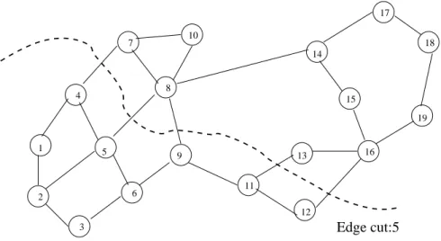
The combinatorial approach (8,9,10,11,12) attempts to group together highly connected ver-tices regardless of location in space. Two well known schemes are Levelized Nested Dissection (LND) and Kernighan-Lin (KL) / Fiduccia-Mattheyses (FM) Algorithm. In Levelized Nes-ted Dissection, an initial vertex is chosen and assigned to level 0. All vertices adjacent to the initial vertex are assigned to level 1. All vertices adjacent to the selected vertices are assigned to the next level. This continues until half of the vertex weight is in the group of selected vertices. The KL / FM algorithm takes as an input a graph that has been par-titioned (sub-optimally) and improves the partition while maintaining load balance of the partitions obtained. The idea in the KL algorithm is to repeatedly find a pair of vertices, one from each sub-domain, and swap their sub-domains. The FM algorithm moves a single vertex at a time. Both algorithms use gain to make decisions regarding the vertices to move, where the gain is the amount by which the edge-cut will decrease if the vertex is moved to the other sub-domain. Figure 3 illustrates the Kernighan Lin method.
Another method of solving the bisection problem is to formulate it as the optimization of a discrete quadratic function. A class of graph partitioning methods called spectral methods (13,14,15), relax this discrete optimization problem by transforming it into a continuous one.
Axe d’inertie minimale
Perpendiculaire a l’axe d’inertie
Fig.1 – Inertial Bissection
1 2 3 4 5 6 7 8 9 10 11 12 13 14 15 16 17 18 19
Edge cut:5
Fig. 3 – Kernighan-Lin Method
The minimization of the relaxed problem is then solved by computing the second eigenvector of the discrete Laplacian of the graph. The first step of this algorithm is to obtain the Lapla-cian matrix of the graph. The LaplaLapla-cian matrix LG of the graph is = A - D (the adjacency matrix - the degree matrix). The second step is to compute the second eigenvector (Fiedler vector) of LG . The Fiedler vector associates a value with each vertex and this value is used later to order the vertices and in the third step the list is split in half. Figure 4 illustrates spectral partitioning approach.
Recently, a new class of partitioning algorithms have been developed based on the multi-level paradigm (16,17,18,19,20). This paradigm consists of three phases : graph coarsening, initial partitioning, and multilevel refinement. In the graph coarsening phase, a series of graphs is constructed by collapsing together selected vertices of the input graph in order to form a related coarser graph. This newly constructed graph then acts as the input graph for another round of graph coarsening, and so on, until a sufficiently small graph is obtained. Computation of the initial bisection is performed on the coarsest (and hence smallest) of these graphs, and so is very fast. Finally, partition refinement is performed on each level graph, from the coarsest to the finest (i.e., original graph) using a KL/FM-type algorithm. Figure 5 presents the multilevel partitioning method.
The partitioning algorithms that we are going to present in this paper can be classified into the combinatorial algorithms category. The objective is to decompose an urban network into sub-networks of limited size such that the number of connections among the sub-networks is minimized. In other words, the traffic flow between the sub-networks is reduced.
Note that the decomposition of sub-networks presented in this paper is used for developing a route guidance system that aids drivers to find out the fastest paths between a given
Input Graph Output Graph 1 5 3 4 2 6 1 5 3 4 2 6
1
1
2 3
4 5
6
2
6
5
4
3
1 2 3 4 5 6
1
2
3
4
5
6
1
2
3
4
5
6
1
2
3
4
5
6
−2
1
1
−2
1
1
−3 1
1
1
1 −3
1
1
1
−2
1
1
−2
1
1
1 1
1
1
1
2
2
3
3
2
2
1
1
1
1
1
1
1
1
L
G= A − D
A
D
Phase
de
réduction
Phase de partition initiale
Phase
de
rafinement
G0 G1 G2 G3 G4 G2 G1 G0 G3origin-destination paper in the following manner : Step 1 :
Find the sequence S0, S1, S2, .., SN, SD of the sub-networks to be visited in order to reach
destination D from an origin O where O ∈ S0and D ∈ SD. This sequence is obtained using
dynamic programming and is based on statistical data. Step 2 :
Computation of fastest paths and the corresponding travel times for the sub-networks ob-tained from step 1. This is done using the decision rules which are generated as a result of statistical analysis on traffic data.
Figure 6 illustrates this approach.
Network Limit Subnetwork boundaries Destination (D) (O) 1 2 3 4 5 6 Origin Global Path Local Path S1 2 S2 3
Fig. 6 – Route guidance approach
Suppose that the step 1 indicates that the vehicle should pass through the points O → S1
2 → S32→ D in order to join O to D. Let us assume that the vehicle is currently at position
O. Therefore, it must exit at point S1
2 in order to leave the current sub-network. At this
stage, we will find out the fastest path between O and S1
2 using the decision rules obtained
from statistical analysis. When the vehicle exits the sub-network 1 and enters sub-network 2, then the fastest path between the entry node S1
2 and exit node S32 is computed. Finally,
the vehicle arrives the sub-network 3 at entry node S2
3 and the fastest path between this
node and the final destination D is computed as explained before. To summarize, we can say that in order to find the fastest path between a given origin-destination pair on a large network, our approach first performs the decomposition of the network into sub-networks,
then computes a global path using dynamic programming in order to obtain the sequence of sub-networks to be visited alongwith their respective entry and the exit points. Finally, the fastest path on the sub-networks also called as the local path is computed using the decision rules obtained from statistical data analysis. In this paper, we will focus only on the decomposition of large scale networks into sub-networks.
2
Recursive Progression - 1 (RP-1)
The first algorithm proposed for decomposition of large scale urban network is called RP-1. It is iterative in nature and partitions the networks into sub-networks recursively. The different characteristics of the algorithm RP-1 are :
2.1
Objective
The criteria’s used in RP-I for decomposing a large network into sub-networks are : 1. The sub-networks should be as least as possible connected to each other. In other
words, we are trying to minimize the number of boundary nodes. These nodes are the points through which a vehicle enters (or leaves) a sub-network.
2. The sub-networks should have limited size.
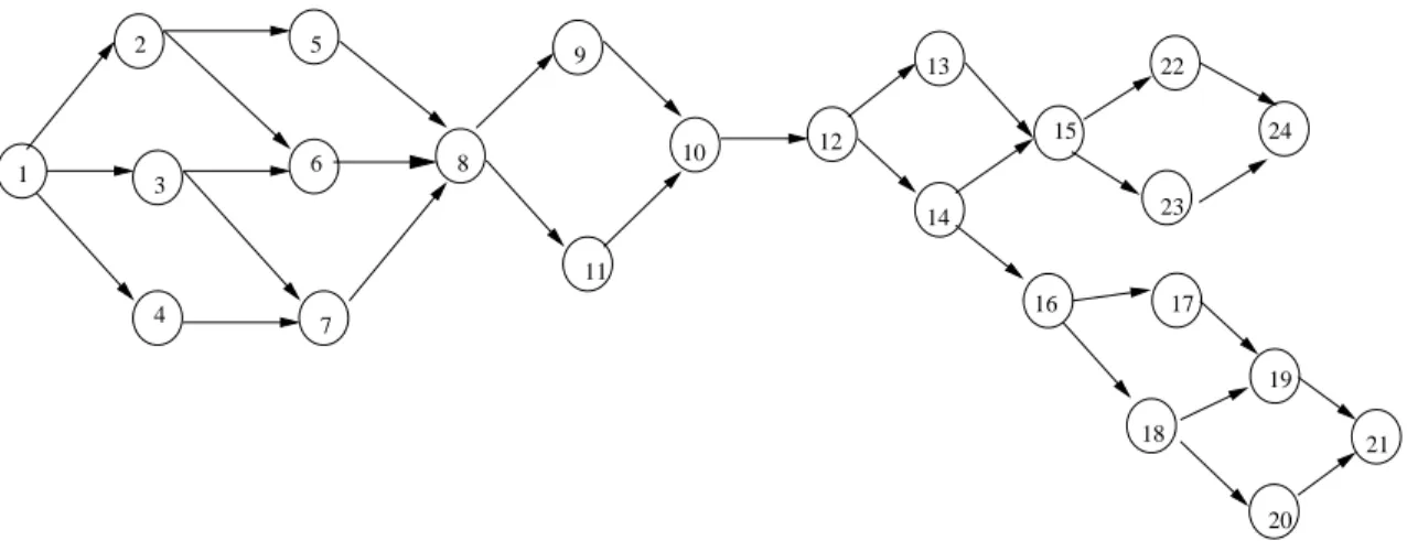
Note that a limitation on the number of boundary nodes is put in order to meet the require-ments of another algorithm namely fastest path algorithm for our route guidance approach. The computational efficiency of this algorithm depends on the number of O-D pairs. Remark :We consider that a boundary node acts as an exit node for one sub-network and an entry node for another sub-network. However, this remark does not applies to the nodes which are the origin or the destination nodes of the network. Let us consider Figure 7.
We can divide this network into two sub-networks namely S1 and S2 where
S1= {1, 2, 3, 4, 5, 6, 7, 8, 9, 10, 11} and S2= {12, 13, 14, 15, 16, 17, 18, 19, 20, 21, 24}.
In this decomposition, node 1 is the entry node and node 10 is the exit node for sub-network S1. For S2, the entry node is 10 and the exit nodes are 21 and 24. Since the boundary node
10 appears in both the sub-networks namely S1and S2, we can also write :
S2= {10, 12, 13, 14, 15, 16, 17, 18, 19, 20, 21, 24}.
2.2
Notations
Let us consider a network of N nodes. If i ∈ {1, 2, ..N }, then P (i) denotes the prede-cessors of i and S(i) denotes the sucprede-cessors of i. If P (i) = φ then i is an entry node of the network. If S(i) = φ, then i is the exit node of the network. The density of a node i, denoted by q(i), represents the number of predecessors or successors nodes of i. In the example of Figure 7 :
P (3) = 1, S(3) = {6, 7}, q(3) = 3.
1 2 3 4 5 6 7 8 9 12 13 14 16 11 10 15 22 23 24 17 18 19 20 21
Fig.7 – A simple Network
density of node 3 is equal to 3/1 = 3.
The density of a sub-network is defined as the ratio of the total number of nodes externally connected to the nodes of the sub-network divided by the total number of nodes present inside the sub-network. If an exterior node is a successor or a predecessor of multiple nodes of the sub-network, then it is counted only once.
For example in Figure 7 :
q(22, 23, 24) = 1/3 because the only predecessor or successor node of this group of nodes is node 15. This is the only exterior node of this group while the group itself contains three nodes. Therefore, the density is equal to 1 divided by 3.
Similarly, the predecessors of a sub-network are defined as the predecessors of all the consti-tuent nodes of the sub-network excluding the predecessor nodes that are present in the group itself. Therefore,
P (8, 9, 10, 11) = {5, 6, 7}. and
S(8, 9, 10, 11) = {12}.
2.3
Methodology
The algorithm RP-1 explores all pair of connected sub-networks at each iteration in order to obtain sub-networks that can be united to form a sub-network which has the minimum density among all the other combinations possible. The properties of the resulting sub-network are :
– It consists of connected sub-networks i.e. at least one arc exists that has its head in one sub-network and the tail in the other sub-network.
– The sum of the number of nodes of the sub-network does not exceed a value provided by the user.
– The density of the sub-network is greater than a value provided by the user. The density of a sub-network is the ratio of the number of nodes externally connected to this sub-network divided by the cardinality of the sub-network. If this density is small, then this sub-network is relatively isolated and we do not try to unite it with other sub-networks. Remember that if we choose a very high density limit, then we force the sub-networks to have a high number of interconnections. This density should therefore be chosen with care. Of course, this density will never exceed 1 because this signifies that we are more interested by the sub-networks that have higher number of external nodes than the internal ones, which is of course not the case.
2.4
Algorithm
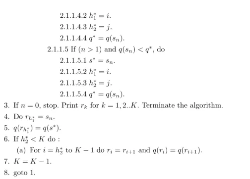
The algorithm RP-1 is presented stepwise as follows : A. Introduction of data
– N : Total number of nodes of the network. – A : Total number of arcs of the network.
– H : {n1, n2, n3, ..nN} group of nodes of the sub-networks.
– Q : Maximum density of a sub-network. By definition, the density of a sub-network rk is given by q(rk) = card(rC(rk)
k) where C(rk) represents the total number of externally
connected nodes of rk and card(rk) represents the cardinality of the sub-network rk.
– W : Maximum number of nodes in a sub-network. B. Initialisation
– K = N .
K is the variable that contains the number of sub-networks at each instant. – For k = 1, 2, ..K, do rk = {k} .
Initially each sub-network consists of a single node. – For k = 1, 2..K, do q(rk) = {card(rC(rk) k)}. C. Computation 1. Do n = 0. 2. For i = 1 to K − 1. 2.1 For j = i + 1 to K.
2.1.1 If (riand rj are connected) and (card(ri) +card(rj) ≤ W ) and (q(ri) > Q)
and (q(rj) > Q) : 2.1.1.1 Do n = n + 1. 2.1.1.2 Do sn= ri∪ rj. 2.1.1.3 Calculate q(sn) = card(sC(sn)n). 2.1.1.4 If (n = 1) do 2.1.1.4.1 s∗= sn.
2.1.1.4.2 h∗ 1= i. 2.1.1.4.3 h∗ 2= j. 2.1.1.4.4 q∗= q(sn). 2.1.1.5 If (n > 1) and q(sn) < q∗, do 2.1.1.5.1 s∗= sn. 2.1.1.5.2 h∗ 1= i. 2.1.1.5.3 h∗ 2= j. 2.1.1.5.4 q∗= q(sn).
3. If n = 0, stop. Print rk for k = 1, 2..K. Terminate the algorithm.
4. Do rh∗ 1 = sn. 5. q(rh∗ 1) = q(s ∗). 6. If h∗ 2< K do : (a) For i = h∗
2to K − 1 do ri= ri+1 and q(ri) = q(ri+1).
7. K = K − 1. 8. goto 1.
Steps 4 to 8 unite two sub-networks at each iteration and replace it by the new sub-network obtained from step 2.
2.5
Numerical Example
Consider the numerical example of Figure 7. N represents the total number of nodes of the network. The maximum number of nodes of each sub-network is denoted by W . K is the variable that contains the number of sub-networks at each iteration of the algorithm. For this example, we have W = 8 and Q = 0.1. Let riand rj be the sub-networks that we unite
at each step (or iteration) in order to obtain a sub-network sn. The cardinality, density and
the number of externally connected nodes of a sub-network ri are denoted by card(ri), q(ri)
and C(ri). The maximum density of a sub-network is denoted by Q. Initially, we have 24
sub-networks each containing a single node. Therefore K = N = 24. At each step, we unite two sub-networks on the basis of the following criteria’s :
– They are connected.
– Their density is greater than Q = 0.1.
– Their reunion leads to a sub-network whose cardinality does not exceeds W = 8. – After grouping, they lead to a sub-network that has minimum density among all the
other combinations possible.
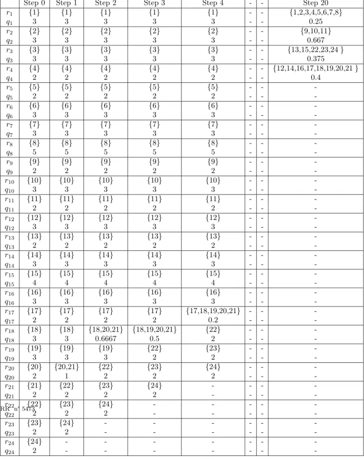
Table 1 presents the results obtained from RP-1.
The initial network data is presented in step 0 or column 2 of table 1. It can be seen that initially there are 24 sub-networks each containing a single node. Two sub-networks are combined consecutively at each iteration using the criteria’s described before. Column 3 presents the results obtained from the first iteration of algorithm RP-1. The sub-networks
Tab.1 – Results obtained from RP-1
Step 0 Step 1 Step 2 Step 3 Step 4 - - Step 20
r1 {1} {1} {1} {1} {1} - - {1,2,3,4,5,6,7,8} q1 3 3 3 3 3 - - 0.25 r2 {2} {2} {2} {2} {2} - - {9,10,11} q2 3 3 3 3 3 - - 0.667 r3 {3} {3} {3} {3} {3} - - {13,15,22,23,24 } q3 3 3 3 3 3 - - 0.375 r4 {4} {4} {4} {4} {4} - - {12,14,16,17,18,19,20,21 } q4 2 2 2 2 2 - - 0.4 r5 {5} {5} {5} {5} {5} - - -q5 2 2 2 2 2 - - -r6 {6} {6} {6} {6} {6} - - -q6 3 3 3 3 3 - - -r7 {7} {7} {7} {7} {7} - - -q7 3 3 3 3 3 - - -r8 {8} {8} {8} {8} {8} - - -q8 5 5 5 5 5 - - -r9 {9} {9} {9} {9} {9} - - -q9 2 2 2 2 2 - - -r10 {10} {10} {10} {10} {10} - - -q10 3 3 3 3 3 - - -r11 {11} {11} {11} {11} {11} - - -q11 2 2 2 2 2 - - -r12 {12} {12} {12} {12} {12} - - -q12 3 3 3 3 3 - - -r13 {13} {13} {13} {13} {13} - - -q13 2 2 2 2 2 - - -r14 {14} {14} {14} {14} {14} - - -q14 3 3 3 3 3 - - -r15 {15} {15} {15} {15} {15} - - -q15 4 4 4 4 4 - - -r16 {16} {16} {16} {16} {16} - - -q16 3 3 3 3 3 - - -r17 {17} {17} {17} {17} {17,18,19,20,21} - - -q17 2 2 2 2 0.2 - - -r18 {18} {18} {18,20,21} {18,19,20,21} {22} - - -q18 3 3 0.6667 0.5 2 - - -r19 {19} {19} {19} {22} {23} - - -q19 3 3 3 2 2 - - -r20 {20} {20,21} {22} {23} {24} - - -q20 2 1 2 2 2 - - -r21 {21} {22} {23} {24} - - - -q21 2 2 2 2 - - - -r22 {22} {23} {24} - - - - -q 2 2 2 - - - - -RR n° 5473
chosen for reunion at step 0 are r20and r21. The sub-networks chosen are r20and r21because
they are connected, their density is greater than 0.1, their reunion leads to a sub-network whose cardinality does not exceeds W (2<8) and whose density leads to the minimum density among all the other densities. Their combination gives rise to sub-network r20 of
column 3. Likewise we can see that in step 2 (column 4) the sub-network r18 is obtained
by the reunion of sub-networks r18 and r20 from step 1. The sub-network r18(column 4)
is composed of three nodes 18,20,21. Therefore W = 3 < 8 and its density = 0.667 which is minimum among all the other densities. In the step 3, the sub-network r18 is obtained
by combination of sub-networks r18 and r19 of step 3. In step 4, the sub-network r17 is
obtained by the grouping of sub-networks r17 and r18 of column 5 (or step 3). Note that
the cardinality of r17 in step 4 is 5 which is less than the permitted value i.e. 8 and has
density = 0.2 which is the minimum among all the other densities. The final results of the algorithm RP-1 are present in the last column of table 1. Four sub-networks namely S1 =
{1,2,3,4,5,6,7,8}, S2 = {9,10,11}, S3 = {13,15,22,23,24} and S4 = {12,14,16,17,18, 19, 20,
21} are obtained. These results are graphically presented in Figure 8.
1 2 3 4 5 6 7 8 9 12 13 14 16 11 10 15 22 23 24 17 18 19 20 21
Subnetwork 1
Subnetwork 2
Subnetwork 4
Subnetwork 3
Fig.8 – Decomposition through RP-1
It can be observed from table 1 and figure 8 that sub-network 1 contains 8 nodes namely 1, 2, 3, 4, 5, 6, 7, 8 and has a density = 0.25. It has one input node namely node 1 and one output node namely node 8. Sub-network 2 contains 3 nodes namely 9,10,11. It has a density equal to 0.667, has one input node namely node 8 and one output node namely node 10. Sub-network 3 contains 5 nodes namely node 13, 15, 22, 23 and 24 and has a density = 0.375. It has two input nodes namely node 13 and 15 and one output node namely node 24.
Finally, we can see that sub-network 4 contains 8 nodes namely 12, 14, 16, 17, 18, 19, 20, 21 and has a density equal to 0.4. It has one input node i.e. node 10 and three output nodes namely nodes 12, 14 and 21.
Note also that at each consecutive iteration we obtain a reduction in the density of the sub-network obtained from reunion. For example, in table 1 we can see that q(r20) = 3 (step
1)> q(r18) = 0.666 (step 2) > q(r18) = 0.5 (step 3) > q(r17) = 0.2(step 4). The algorithm
stops after 20 iterations because it is no more possible to find a couple of sub-networks which are :
– connected,
– Will lead, after union, to a sub-network whose cardinality will not exceed 8, – Will lead, after union, to a sub-network whose density remains greater than 0.1. We emphasize that in the algorithm RP-1, the density is calculated not on the basis of boundary nodes, but on the number of connections with other sub-networks.
2.6
Algorithm Analysis.
2.6.1 Complexity.
The complexity of the algorithm HRP presented here is its worst case complexity. It is calculated in two steps as follows :
1. Calculation of the complexity of each step. 2. Calculation of the total complexity.
Assume that the step A of HRP entitled ‘Introduction of data’ takes t1 units of time. The
step B of algorithm HRP entitled ‘Initialisation’ takes 1 + Nt02 + Nt”2 where t
0
2 and t”2 are
the times for the initialisation of rk and q(rk) respectively. In the step C entitled
‘Computa-tion’, the steps number 1,4,5,7,8 each take 1 unit of time (sum = 5 units of time). Since the computations of step 2 are executedPNi=1N − i = N(N −1)2 times, therefore the computation time for step 2 is N(N −1)2 t3 assuming that each loop of step 2 takes t3 units of time. The
computation times for step 3 and step 6 are Nt4 and (N-1)t5 where t4 represents the time
required for printing the sub-networks obtained at the end of step 2 and t5 represents the
time for computing the size and the density of sub-networks obtained by the integration of two sub-networks at each iteration.
Since step C can be executed to a maximum of N times, therefore the total complexity of the algorithm HRP is :
N (1 + N t02+ N t”2+ 5 +
N (N − 1)
2 t3+ N t4+ (N − 1)t5) = O(N
3)
Therefore, in the worst case, the complexity of the algorithm RP-1 is O(N3), where N is the
2.6.2 Properties.
At each iteration, the algorithm RP-1 unites the pair of sub-networks which meet the following conditions :
– They are connected.
– The total number of nodes in each sub-network do not exceed a given limit, namely W as shown in the numerical example of section 2.5.
– The density of both the sub-networks is greater than a limit, which lies between 0 and 1. It is noted Q in the numerical example of section 2.5.
The algorithm then combines the two sub-networks whose union leads to the minimum density.
The algorithm contains N sub-networks (one node per sub-network) at the start and loses one sub-network at each consecutive series of iterations, it will converge necessarily when no iterations would be possible, i.e. when there exists no more pairs of sub-networks whose cardinalities are less than or equal to W and whose densities remain greater than or equal to Q. This gives rise to the following properties :
Property 1:
The algorithm RP-1 converges after a certain number of iterations. This number is less than or equal to N−1.
Proof :In algorithm HRP, two sub-networks are combined at each iteration to form a new sub-network whose size and density constraints do not exceed a value predefined by the user. The algorithm terminates when either size constraint or density constraint or both the size and density constraints of resulting sub-network are violated. Since, this situation can occur at the earliest after the first iteration (i.e. 1) or at the most at the last (i.e. N−1) iteration. Hence, the number of iterations required for the convergence of algorithm HRP is less than or equal to N−1. This proves the property 1.
Property 2:
Let r1 and r2 represent two sub-networks and s = r1∪ r2. We denote q(x) as the density of
a sub-network x. We suppose that the number of exterior nodes connected to s is equal to the sum of the number of exterior nodes of r2 which are connected to r1 and the number of
exterior nodes of r1 which are connected to r2.
Then :
q(s) ≤ M ax{q(r1), q(r2)}
Proof : We denote :
a1,2 : Total number of nodes of r2 which are connected with nodes of r1.
a2,1 : Total number of nodes of r1 which are connected with nodes of r2.
n1,2 : Total number of exterior nodes of r2 which are connected with nodes of r1.
n2,1 : Total number of exterior nodes of r1 which are connected with nodes of r2.
N1 : Total number of nodes in r1.
N2 : Total number of nodes in r2.
Then : q(r1) = a1,2+ n1,2 N1 ; q(r2) = a2,1+ n2,1 N2 q(s) = ms,s N1+ N2 with ms,s= n1,2+ n2,1
Let us assume that q(r1) < q(s). This leads to :
(N1+ N2)a1,2+ N1n1,2+ N2n1,2− ms,sN1< 0
But m = n1,2+ n2,1, therefore :
(N1+ N2)a1,2+ N2n1,2− N1n2,1< 0 (1)
Similarly, using q(r2) < q(s), we obtain :
(N1+ N2)a2,1+ N1n2,1− N2n1,2< 0 (2)
Suppose that (1) holds true. Then, N1n2,1 > N2n1,2 is not possible for (2) and vice versa.
Consequently, we cannot obtain simultaneously q(r1) < q(s) and q(r2) < q(s), which proves
the results. Corollary
The maximum density of a group of sub-networks reduces inversely with the number of iterations of the algorithm. The reason is the number of internal nodes of the resulting sub-network increases and the number of externally connected nodes decreases at each iteration. The density of the resulting sub-network is less than or equal to the maximum density among the densities of the two combining sub-networks at each iteration as proved in property 1. The property (3) completes the previous ones.
Property 3:
Using the previous notations and assuming that ms,s= n1,2+ n2,1 :
1. q(s) ≤ q(r1) and q(s) ≤ q(r2) if
|N2n1,2− N1n2,1| < (N1+ N2)M in(a1,2, a2,1).
2. If the previous condition is not verified, and if a1,2= a2,1, then :
2.1 q(r1) < q(s) ≤ q(r2) iff NN2 1 < n 2,1 n 1,2. 2.2 q(r2) < q(s) ≤ q(r1) iff NN1 2 < n 1,2 n 2,1. Proof :
1. After (1), q(r1) ≥ q(s) if and only if :
(N1+ N2)a1,2+ N2n1,2− N1n2,1≥ 0
Similarly from (2), q(r2) ≥ q(s) if and only if :
These two relations are always verified if :
|N2n1,2− N1n2,1| < (N1+ N2)M in(a1,2, a2,1)
Hence, proved.
2. q(r1) < q(s) if and only if (1) is verified.
q(r2) ≥ q(s) if and only if :
(N1+ N2)a2,1+ N1n2,1− N2n1,2≥ 0 (3)
By subtracting (1) from (3) and taking into account that a1,2= a2,1, we obtain :
N1n2,1− N2n1,2 > 0 Or : N2 N1 = n2,1 n1,2 The condition (2) can be explained in an identical way. Remark :Assuming that the following properties are verified i.e.
1. Symmetric : a1,2= a2,1.
This property signifies that the number of connections of sub-network r1with another
sub-network r2 is equal to the number of connections of r2 with r1.
2. Additivity : ms,s= n1,2+ n2,1.
This property signifies that, when two sub-networks are combined, then the number of exterior links of the resulting sub-network is equal to the sum of the exterior links of the two sub-networks minus two times the links between these two sub-networks, Then : a). q(s) ≤ M ax{q(r1), q(r2)} (4) b). q(s) ≤ q(r1) et q(s) ≤ q(r2) iff |N2n1,2− N1n2,1| < (N1+ N2)a1,2 (5) c). q(r1) < q(s) ≤ q(r2) iff NN2 1 < n 2,1 n 1,2 (6) d). q(r2) < q(s) ≤ q(r1) iff NN1 2 < n 1,2 n 2,1 (7)
The conditions hold true if a ‘link’ between the sub-networks represents the number of arcs that connect these sub-networks.
The property (4) gives the information about the maximum number of sub-networks obtai-ned for a given value of W .
Property 4
The maximum number (p) of sub-networks obtained if the initial network contains N nodes and if the size of a sub-network does not exceeds W is given by p = bN
Wc, where bac is the
integer number lesser than or equal to a.
Proof :If p represents the number of sub-networks, then we can form C2
total number of occurrence of a node in such couple is p − 1. As a result, if we add the number of nodes in these couples, we obtain (p − 1)N . But, the sum of the number of nodes in the elements of a couple is less than W , which leads to the following inequality :
Cp2W < (p − 1)N
By developing and studying this equation of second degree, we obtain p = bN Wc.
3
Recursive Progression - 2 (RP-2)
The difference between the algorithms RP-1 and RP-2 lies in the way through which two sub-networks are combined at each iteration.
In RP-1, the system searches two sub-networks whose reunion will lead to a minimum density sub-network.
In RP-2, the system searches the network of maximum density, then searches the sub-network with the second largest density to which it is connected and such that :
– The resulting sub-network obtained from their union has a size less than or equal to the maximum permitted size.
– The resulting sub-network has minimum density than the individual densities of the two sub-networks.
3.1
Algorithm
1. Data Introduction 1.1 Introduce N .
N is the total number of nodes of the network. 1.2 For i = 1, 2, ..N
1.2.1 Introduce si.
si is the number of successors of i.
1.2.2 For k = 1, 2, ..si, introduce lsi,k.
lsi,k is the list of successors of i.
1.3 For i = 1, 2, ..N
1.3.1 Compute the number of predecessors of i i.e. pi.
1.3.2 For k = 1, 2, .., pi, introduce the predecessors in the list lpi,k.
2. Initialisation
2.1 For i = 1, 2, ..N , do : 2.1.1 qi= si+ pi
Since each sub-network consists of a single node at the start of the algorithm, therefore qi initially represents the number of external connections of i. In the
rest of the program, qi denotes the number of connections of ith element of the
2.1.2 nbi= 1.
nbi is initially equal to 1 because each element of the list is composed of a single
node. 2.1.3 ei,1= i.
This is the first element of the ith sub-network (initially).
3. Search of the sub-network with the maximum density 3.1 x = 0.
x contains the maximum density (if it exists). 3.2 cont = 0.
cont is a flag that will be equal to 1 if a sub-network has “admissible” density, i.e. its density is greater than a given density and the size is less than a given size is identified. 3.3 For i = 1, 2, ..N , do :
3.3.1 : w = qi/nbi.
w is the density of the ith element.
3.3.2 : If (w > x) and (nbi< W ) and (w > Q) do :
3.3.2.1 cont = 1. 3.3.2.2 i1 = i. 3.3.2.3 x = w.
We search therefore a sub-network of maximum density : a).whose size does not exceeds W
b).whose density is greater than Q.
i1 is the position of the sub-network retained and, simultaneously it is the identificator
of the first node of this sub-network. 3.4 If cont = 0, end. Print the results. 4. Search of the elements to be grouped
4.1 Do j1= −1 and x = 0.
4.2 Search among the successors of i1.
4.2.1 For j = 1 to si1 do : 4.2.1.1 r = lsi1,j. 4.2.1.2 w = qr/nbr. 4.2.1.3 If (w > x) and (nbi1+ nbr<= W ) do : 4.2.1.3.1 j1= r. 4.2.1.3.2 x = w.
We group the maximum density sub-network with another connected sub-network ha-ving the following properties :
a). It has the largest density.
b). After grouping with this sub-network, the resulting sub-network does not exceeds the maximum size ‘ma’.
5. If j1= −1, print the results. Terminate the algorithm.
6. Regrouping of two sub-networks 6.1 Creation of new list of successors. 6.2 Creation of new list of predecessors.
6.3 Creation of the list of nodes of the new sub-network.
6.4 Put the new sub-network obtained from reunion in the place of the constituent sub-network having lower position in the list.
6.5 Delete the constituent sub-network which is at a higher position in the list. 6.6 N = N − 1.
6.7 goto 3.
Remark : The algorithm terminates if all the sub-networks have a density greater than a predefined density and a size less than a predefined size. Note that the size condition is always verified in the algorithm. We have however introduced two different limits. The size limit has higher priority over the density limit.
The algorithm terminates equally when, after a sub-network is chosen, it is not possible to find a sub-network which is connected to it and does not possesses the following properties :
– The sub-network has a density greater than a given value.
– Its association with initial sub-network leads to a sub-network with size lesser than a given value (superior ou equal to previous one).
3.2
Numerical example
Let us consider the numerical example of Figure 7. The total number of nodes of the network is denoted by N and the maximum number of nodes in a sub-network is denoted by W . K represents the variable that contains the number of sub-networks at each iteration. In the example, W = 8 and Q = 0.1. Let ri be the elements or the sub-networks that we
group at each iteration to obtain sn. The cardinality, density and the number of exterior
nodes of the sub-network ri are denoted by card(ri), q(ri) and C(ri). The maximum density
of a sub-network is denoted by Q. Initially, we have 24 sub-networks each containing single node. Therefore K = N = 24. This situation is presented in the column 1 or step 0 of table 2. It can be seen in step 1 (column 3) of table 2 that sub-network r6 is obtained by
the combination of sub-networks r6 and r8 of column 2. These sub-networks are combined
because they are connected, their density is higher than 0.1, and they have the highest and the second highest density respectively. Similarly in step 2 (column 4), the sub-network r14 is obtained from the union of sub-networks r14 and r15 of step 1. In the step 3, r2
is obtained by combination of sub-networks r2 and r6 of step 2. In the fourth step, r1 is
obtained by the grouping of sub-networks r1and r3of step 3 i.e. fifth column. The algorithm
terminates after 20 iterations to yield four sub-networks namely S1= {1,2,3,4,5,6,7,8},S2=
{9,10,11,12,13,14}, S3 = {22,23,24} and S4 = {16,17,18,19,20,21}. These sub-networks are
graphically represented in Figure 9.
It can be seen in figure 9 that sub-network 1 contains 8 nodes namely 1, 2,3,4,5,6,7,8 and has a density = 0.375. It has one input node namely node 1 and one output node namely
1 2 3 4 5 6 7 8 9 12 13 14 16 11 10 15 22 23 24 17 18 19 20 21
Subnetwork 2
Subnetwork 4
Subnetwork 3
Subnetwork 1
Tab.2 – Results obtained from RP-2
Step 0 Step 1 Step 2 Step 3 Step 4 - - Step 20 r1 {1} {1} {1} {1} {1,3} - - {1,2,3,4,5,6,7,8 } q1 3 3 3 3 2 - - 0.375 r2 {2} {2} {2} {2,6,8} {2,6,8} - - {9,10,11,12, 13,14,15 } q2 3 3 3 2.3333 2.3333 - - 0.25 r3 {3} {3} {3} {3} {4} - - {22,23,24} q3 3 3 3 3 2 - - 0.667 r4 {4} {4} {4} {4} {5} - - {16,17,18,19,20,21} q4 2 2 2 2 2 - - 0.4 r5 {5} {5} {5} {5} {7} - - -q5 2 2 2 2 3 - - -r6 {6} {6,8} {6,8} {7} {9} - - -q6 3 3 3 3 2 - - -r7 {7} {7} {7} {9} {10} - - -q7 3 3 3 2 3 - - -r8 {8} {9} {9} {10} {11} - - -q8 5 2 2 3 2 - - -r9 {9} {10} {10} {11} {12} - - -q9 2 3 3 2 3 - - -r10 {10} {11} {11} {12} {13} - - -q10 3 2 2 3 2 - - -r11 {11} {12} {12} {13} {14,15} - - -q11 2 3 3 2 2.5 - - -r12 {12} {13} {13} {14,15} {16} - - -q12 3 2 2 2.5 3 - - -r13 {13} {14} {14,15} {16} {17} - - -q13 2 3 2.5 3 2 - - -r14 {14} {15} {16} {17} {18} - - -q14 3 4 3 2 3 - - -r15 {15} {16} {17} {18} {19} - - -q15 4 3 2 3 3 - - -r16 {16} {17} {18} {19} {20} - - -q16 3 2 3 3 2 - - -r17 {17} {18} {19} {20} {21} - - -q17 2 3 3 2 2 - - -r18 {18} {19} {20} {21} {22} - - -q18 3 3 2 2 2 - - -r19 {19} {20} {21} {22} {23} - - -q19 3 2 2 2 2 - - -r20 {20} {21} {22} {23} {24} - - -q20 2 2 2 2 2 - - -r21 {21} {22} {23} {24} - - - -q21 2 2 2 2 - - - -r22 {22} {23} {24} - - - - -q 2 2 2 - - - -
-node 8. Sub-network 2 contains 7 -nodes namely 9,10,11,12,13,14 and 15. It has a density equal to 0.25, has one input node namely node 8 and two output nodes namely node 14 and 15. Sub-network 3 contains 3 nodes namely node 22, 23 and 24 and has a density = 0.667. It has one input node namely node 15 and one output node namely node 24. Finally, we can see that sub-network 4 contains 6 nodes namely 16,17,18,19,20,21 and has a density equal to 0.4. It has one input node i.e. node 16 and one output node i.e. node 21.
3.3
Algorithm Analysis
3.3.1 Complexity of the algorithm.
We are going to first calculate the complexity of each step of algorithm RP-2 and then its total complexity.
Let us consider the algorithm RP-2. The step 1 of the algorithm RP-2 entitled ‘Introduction of data’ takes 1+ Nt01 + Nt
00
1 units of time, where we assume that t
0
and t” are the times
required for the introduction of the list of successors and predecessors of N initial sub-networks. The step 2 entitled ‘Initialisation’ takes 3N units of time for the initialisation of the elements and the connections of each sub-network. In the third stage C entitled ‘Search of the sub-network with the maximum density’, the computation time for 3.1 and 3.2 is 1 units each. Suppose that t2 is the time required for searching the sub-network of maximum
density in step 3.3 and t3 is the time required for printing the results of step 3.4. Since the
steps 3.3 and 3.4 can be executed to a maximum of N times, the complexity is 2+Nt2+ Nt3
for the third step of algorithm RP-2. Suppose that step 4 takes t4units of time, step 5 takes
N units of time and the steps 6.1-6.5 take t5units of time. It is clear that steps 6.6-6.7 take
1 units of time each (total = 2).
Since the loop containing the steps 3-6 is executed maximum N times, the total complexity of the algorithm RP-2 is given by :
N (1 + N t01+ N t”1+ 3N + 2 + N t2+ N t3+ t4+ N + t5+ 2) = O(N2)
Therefore, the complexity of algorithm RP-2 in the worst case is O(N2), where N is the
total number of nodes of the network. 3.3.2 Properties of the algorithm.
In RP-2, the density of a sub-network is calculated as the ratio of the number of externally connected arcs of this network divided by the cardinality of the sub-network. The definition of density is therefore different between RP-1 and RP-2, although, in practice, these two definitions are close to each other. The advantage of this new definition of density is that the properties of symmetry and additivity introduced in the section 2.6 are verified. As a result, the properties (4),(5),(6) and (7) are also verified.
Tab.3 – Application of RP-1 on first three networks Network Number of Number of Number of Density
Id nodes input nodes exit nodes
1 10 9 9 1.3 10 6 7 0.6 10 9 6 1 10 7 8 0.7 1 3 1 5 6 6 5 2.3333 1 1 1 0 1 1 1 1 1 3 1 6 2 10 5 5 0.7 9 10 5 1.7778 10 7 4 0.6 10 9 7 1.1 10 5 5 0.6 1 1 1 0 3 10 7 7 0.6 2 3 1 2 10 6 10 1.1 10 6 5 0.8 10 3 6 0.8 2 4 1 2 2 2 2 3.5 1 5 1 8 1 1 1 0 1 2 1 2 1 3 1 6
4
Comparison between RP-1 and RP-2.
Tables 3 and 4 present the results obtained by the application of the algorithms RP-1 and RP-2 on networks of 50 nodes generated at random.
We have generated the networks at random as follows : – Number of nodes : 50.
– Number of successors of a node : between 0 and 3.
– Number of experiments : 50 (We have retained only first 3 experiment results in the tables 3 and 4).
Tab.4 – Application of RP-2 on first three networks Network Number of Number of Number of Density
Id nodes input nodes exit nodes
1 10 7 9 1.7 10 11 7 1.7 10 11 8 1.6 10 7 8 1.5 1 1 1 1 1 1 1 1 1 1 1 1 1 1 1 1 1 1 1 1 1 1 1 1 3 2 2 0.3333 1 1 1 0 2 10 15 9 3.2 1 1 1 2 3 4 2 1.6667 10 9 7 1.6 2 2 2 1.5 2 1 2 1.5 1 1 1 1 1 1 1 1 1 1 1 1 1 1 1 1 1 1 1 1 7 5 4 0.857143 7 3 4 0.714286 2 1 1 0.5 1 1 1 0 3 10 12 9 3.3 1 3 1 3 1 1 1 2 1 1 1 2 4 2 4 1.75 10 7 7 1.7 7 5 4 1.28571 1 1 1 1 1 1 1 1 3 2 1 0.666667 10 7 7 0.6 1 1 1 0
– Q = 0.1.
Note that the program for generation of graphs tries to eliminate neither the isolated nodes nor the cycles. In other terms, the graph obtained can be cyclic and non-connex.
We observe from tables 3 and 4 that the algorithm RP-2 produces much more isolated nodes than the algorithm RP-1. The reason is that certain nodes cannot be included in the sub-networks due to limitation on the size or the maximum number of nodes in each sub-network. We found that the sub-networks obtained by the algorithm RP-1 cover better the network than the algorithm RP-2, which assures a more homogeneous partition. The algorithm RP-1 is therefore more efficient than RP-2 though at a cost of higher number of computations (see the complexity of these two algorithms in subsections 2.6.1 and 3.3.1). Note that this observation might change if these algorithms are applied on networks of very big size (more than 200 nodes).
Note that the algorithm RP-2 imposes a restriction in one particular situation. The situation occurs when a largest density sub-network is not able to absorb a connected sub-network due to the violation of sub-network size. In that case, the algorithm is forced to stop without generating the partitions. However this situation can be overcome by considering the sub-network with the second largest density for grouping in the algorithm.
5
Decomposition of the Paris network.
Two algorithms namely RP-1 and RP-2 were applied on a part of Paris (Figure 10). The input parameters are N = 690, W = 40, Q = 0.8. The results of the algorithms RP-1 and RP-2 on the Paris network are presented in the Figures 11 and 12 respectively.
In the figures 11 and 12, the colours are used to distinguish the sub-networks. Two sub-networks of same colour but non-connected indicate two different sub-networks. RP-1 algorithm yields 109 sub-networks whereas RP-2 yields 98 sub-networks.
It was observed that the algorithm RP-2 produces more isolated nodes than RP-1. The reason is that certain sub-networks cannot be grouped with other sub-networks due to the limitation imposed on the number of nodes of a sub-network (W = 40) and on the density ( ≥ 0.8) of a sub-network. We observed that if we eliminate the constraints on the density, i.e. if we simply use density Q ≥ 0, then the number of sub-networks obtained are less in number than the case when q = 0.8.
6
Conclusion.
Two algorithms namely RP-1 and RP-2 based on different definitions of density are proposed for partitioning of large scale urban network into sub-networks. In the algorithm RP-1, at each iteration the sub-networks are combined on the basis of connectivity and reduction of density criteria. The density of a sub-network being equal to the number of externally connected nodes of a sub-network divided by its cardinality. In the algorithm RP-2, we group sub-networks that are connected and have high densities. The density being equal
to the number of externally connected arcs divided by the cardinality of the sub-network. The worst case complexity of the algorithm RP-1 is O(N3) whereas that of algorithm RP-2
is O(N2), where N represents the number of nodes of the network. During the study it was found that the sub-networks obtained from RP-1 are more homogeneous than RP-2 though at a cost of higher number of computations.
Improvements in the current algorithms can be done in two ways : 1. Usage of another definition of density. For example :
Density = (total of the input flows and the output flows)/(flows inside the network). 2. Elimination of the constraint on the size of the sub-network, i.e using only the density
criteria for sub-networks. This will permit us to control better the number of entry and exit points of the sub-networks.
The next step of our work concerns the application of this work for finding fastest paths on large scale urban networks.
Références
[1] M. Berger and S. Bokhari. Partitioning strategy for nonuniform problems on multipro-cessors. IEEE Transactions on Computers, C-36(5) :570-580, 1987.
[2] J. Gilbert, G. Miller, and S. Teng. Geometric mesh partitioning : Implementation and experiments. In Proceedings of International Parallel Processing Symposium, 1995. [3] M. Heath and P. Raghavan. A Cartesian parallel nested dissection algorithm. SIAM
Journal of Matrix Analysis and Applications, 16(1) :235-253, 1995.
[4] G. Miller, S. Teng, W. Thurston, and S. Vavasis. Automatic mesh partitioning. In A. George, John R. Gilbert, and J. Liu, editors, Sparse Matrix Computations : Graph Theory Issues and Algorithms. IMA Volumes in Mathematics and its Applications. Springer-Verlag, 1993.
[5] A. Patra and D. Kim. Efficient mesh partitioning for adaptive hp finite element methods. In International Conference on Domain Decomposition Methods, 1998.
[6] J. Pilkington and S. Baden. Partitioning with space filling curves. Technical Report CS94-349, Dept. of Computer Science and Engineering, Univ. of California, 1994. [7] P. Raghavan. Line and plane separators. Technical Report UIUCDCS-R-93-1794,
De-partment of Computer Science, University of Illinois, Urbana, IL 61801, February 1993. [8] C. Ashcraft and J. Liu. A partition improvement algorithm for generalized nested dis-section. Technical Report BCSTECH-94-020, York University, North York, Ontario, Canada, 1994.
[9] J. Gilbert, G. Miller, and S. Teng. Geometric mesh partitioning : Implementation and experiments. In Proceedings of International Parallel Processing Symposium, 1995. [10] T. Goehring and Y. Saad. Heuristic algorithms for automatic graph partitioning.
[11] B. Kernighan and S. Lin. An efficient heuristic procedure for partitioning graphs. The Bell System Technical Journal, 49(2) :291-307, 1970.
[12] P. Sadayappan and F. Ercal. Mapping of finite element graphs onto processor meshes. IEEE Transactions on Computers,C-36 :1408-1424, 1987.
[13] B. Hendrickson and R. Leland. An improved spectral graph partitioning algorithm for mapping parallel computations. SIAM Journal of Scientific Computing, 16(2) :452-469, 1995.
[14] A. Pothen, H. Simon, and K. Liou. Partitioning sparse matrices with eigenvectors of graphs. SIAM Journal of Matrix Analysis and Applications, 11(3) :430-452, 1990. [15] A. Pothen, H. Simon, L. Wang, and S. Barnard. Towards a fast implementation of
spectral nested dissection. In Supercomputing ’92 Proceedings, pages 42-51, 1992. [16] A. Gupta. Fast and effective algorithms for graph partitioning and sparse matrix
reor-dering. IBM Journal of Research and Development, 41(1/2) :171-183, 1996.
[17] B. Hendrickson and R. Leland. A multilevel algorithm for partitioning graphs. Procee-dings Supercomputing ’95, 1995.
[18] G. Karypis and V. Kumar. A fast and high quality multilevel scheme for partitioning irregular graphs. SIAM Journal on Scientific Computing, 20(1) :359-392, 1998.
[19] G. Karypis and V. Kumar. Multilevel k-way partitioning scheme for irregular graphs. Journal of Parallel and Distributed Computing, 48(1), 1998.
[20] B. Monien, R. Preis, and R. Diekmann. Quality matching and local improvement for multilevel graph-partitioning. Technical report, University of Paderborn, 1999.
[21] J. Pilkington and S. Baden. Partitioning with space filling curves. Technical Report CS94-349, Dept. of Computer Science and Engineering, Univ. of California, 1994.
Unité de recherche INRIA Lorraine : LORIA, Technopôle de Nancy-Brabois - Campus scientifique 615, rue du Jardin Botanique - BP 101 - 54602 Villers-lès-Nancy Cedex (France)
Unité de recherche INRIA Rennes : IRISA, Campus universitaire de Beaulieu - 35042 Rennes Cedex (France) Unité de recherche INRIA Rhône-Alpes : 655, avenue de l’Europe - 38330 Montbonnot-St-Martin (France) Unité de recherche INRIA Sophia Antipolis : 2004, route des Lucioles - BP 93 - 06902 Sophia Antipolis Cedex (France)