Coupling analysis of high Q resonators in add-drop configuration through cavity ringdown spectroscopy

(1)

HAL Id: hal-01940112

https://hal.archives-ouvertes.fr/hal-01940112

Submitted on 12 Mar 2020

HAL is a multi-disciplinary open access

archive for the deposit and dissemination of

sci-entific research documents, whether they are

pub-lished or not. The documents may come from

teaching and research institutions in France or

abroad, or from public or private research centers.

L’archive ouverte pluridisciplinaire HAL, est

destinée au dépôt et à la diffusion de documents

scientifiques de niveau recherche, publiés ou non,

émanant des établissements d’enseignement et de

recherche français ou étrangers, des laboratoires

publics ou privés.

Coupling analysis of high Q resonators in add-drop

configuration through cavity ringdown spectroscopy

Gabriele Frigenti, Mojtaba Arjmand, Andrea Barucci, Francesco Baldini,

Simone Berneschi, Daniele Farnesi, Mariagiovanna Gianfreda, Stefano Pelli,

Silvia Soria, A Aray, et al.

To cite this version:

Gabriele Frigenti, Mojtaba Arjmand, Andrea Barucci, Francesco Baldini, Simone Berneschi, et al..

Coupling analysis of high Q resonators in add-drop configuration through cavity ringdown

spec-troscopy. Journal of Optics, Institute of Physics (IOP), 2018, 20 (6), pp.065706.

�10.1088/2040-8986/aac459�. �hal-01940112�

(2)

Coupling analysis of high Q resonators in

add-drop conﬁguration through cavity ringdown

spectroscopy

G Frigenti

1,2,6

, M Arjmand

3

, A Barucci

1

, F Baldini

1

, S Berneschi

1

,

D Farnesi

1

, M Gianfreda

4

, S Pelli

1

, S Soria

1

, A Aray

3

, Y Dumeige

5

,

P Féron

5

and G Nunzi Conti

1

1_{IFAC-CNR, Institute of Applied Physics ‘Nello Carrara’, National Research Council, Via Madonna del Piano 10, I-50019 Sesto}

Fiorentino (FI), Italy

2_{Laboratorio Europeo di Spettroscopia (LENS), Università degli Studi di Firenze via Nello Carrara 1, 150019 Sesto F.no, Firenze, Italy} 3_{Optics and Laser Sciences & Technology Research Center, Malek-Ashtar University of Technology, 83145-13115, Shahin-Shahr,}

Isfahan, Iran

4_{Centro Fermi - Museo Storico della Fisica e Centro Studi e Ricerche ‘Enrico Fermi’, Piazza del Viminale 1, I-00184 Roma, Italy} 5_{FOTON (CNRS - UMR 6082), Université de Rennes 1, ENSSAT, 6 rue de Kerampont, F-22300 Lannion, France}

E-mail:[email protected]

Abstract

An original method able to fully characterize high-Q resonators in an add-drop configuration has been implemented. The method is based on the study of two cavity ringdown (CRD) signals, which are produced at the transmission and drop ports by wavelength sweeping a resonance in a time interval comparable with the photon cavity lifetime. All the resonator parameters can be assessed with a single set of simultaneous measurements. We first developed a model describing the two CRD output signals and a fitting program able to deduce the key parameters from the measured profiles. We successfully validated the model with an experiment based on a fiber ring resonator of known characteristics. Finally, we characterized a high-Q, home-made, MgF₂whispering gallery mode disk resonator in the add-drop configuration, assessing its intrinsic and coupling parameters.

Keywords: optical resonators, microcavities, whispering gallery mode resonators, ﬁber optics, cavity ringdown spectroscopy

1. Introduction

Whispering gallery mode(WGM) resonators are a family of resonators with curved dielectric interfaces with cylindrical symmetry that allow guiding light in two directions by total internal reﬂection on a quasi-circular path. There are many possible shapes for them, like rings, toroids, spheres and disks, and, if they are made in low loss materials and have a small footprint(few millimetres or below), they can share the

common feature of having very high quality factors and little modal volumes. These characteristics make them interesting for fundamental studies, for instance, in non-linear optics, and for practical applications, like sensing and optical processing. In all cases, being able to characterise the intrinsic properties of the WGM resonator and its interactions with the input-output couplers becomes an important requirement.

The general procedure to couple light to a WGM reso-nator is to use the evanescent tail of a bus waveguide or a prism, which has to be phase matched and partially over-lapped to the WGM[1].

6

(3)

In particular, we realise an add-drop configuration by coupling the WGM resonator to two tapered fibers, therefore having a two coupler and a four port device. The add-drop configuration is very important for a number of studies based on ultra-high-Q WGM microresonators that have recently gained great interest, including, for instance, the implementation of innovative compact Kerr frequency combs[2–5], the generation

of non linear parametric[6,7] and non-parametric [8,9]

oscil-lations, the stabilization of semiconductor lasers operating in the resonators transparent wavelength range[10–12], or the

mode-locking of fast pulsed lasers[13]. In these experiments, where

the frequency conversion through non-linear effects(as well as laser oscillations[14]) is accomplished within the resonators, the

add-drop conﬁguration allows us to efﬁciently collect the signal through the drop channel, while keeping the residual pump on the transfer channel.

The conﬁguration investigated in this work is also very useful for practical applications in which the add-drop con-ﬁguration is the core optical unit for devices like innovative ultra-compact RF optoelectronic oscillators [3, 15, 16] or

ultra-narrowﬁlters [17] and non-linear switches [18–21].

Indeed, being able to completely characterize such WGM resonator based systems is a key step for understanding basic studies as well as for implementing and optimising the per-formances of new devices.

The main motivation for this work has been to implement an original technique based on cavity ringdown spectroscopy (CRDS) which is capable of uniquely assessing the various parameters of a WGM resonator in the add-drop conﬁguration by using a single set of measurements. CRD based techniques may, similar to cavity ringup(CRU) [22], allow us to assess

intrinsic fundamental properties of the resonators, thanks to their high speed processing capabilities[23,24].

2. Model

The sketch shown in figure 1 represents the typical two-waveguides configuration, or add-drop configuration, where a resonator, depicted as a green disk, is coupled to two wave-guides, depicted as blue straight lines in its proximity. The coupling between these elements is graphically represented by two red dashed rectangles and allows light exchange between the waveguides and the resonator. Finally, a set of arrows depicts the direction of light propagation, with the output branches of the two waveguides named the transfer channel and drop channel.

The monochromatic input wave is assumed to be linearly scanned in frequency: depending on the value of the fre-quency scan speedVs, the output traces can be very different.

If Vs is below a threshold scanning speed Vsthr, the

reso-nator excitation is stationary (or adiabatic), and the trans-mission spectrum of the resonator is formed by a series of dips for the transfer channel and a series of spikes for the drop channel (section2.1). Instead, if Vs Vs

thr

> , the traces feature oscillations of decreasing amplitude and period (cavity ring-down regime, section2.2).

The value of V_sthr can be intuitively estimated as the scanning velocity that produces a resonance crossing time

V

FWHM s

thr_{equal to the photon lifetime inside the resonator}

(t ), i.e. [tot 25] Vsthr 2 . tot 2 pt =

In the following, we resume the results and the limits related to stationary regime measurements (section2.1) and

then describe the model developed to predict the transfer and drop signals in the CRD regime(section2.2). In both cases,

we assume that only one mode is excited in both the resonator and the waveguide, ignoring multimode propagation [26].

However, we do not make any assumptions on the speciﬁc features of the resonator or the waveguide, so that the model can be general and can describe any type of waveguide-resonator combination.

2.1. Stationary profiles

Following the coupling matrix formalism described in [27],

we introduce the two unitary matrices Uup and Udown to

mathematically describe the coupling between the resonator and the waveguides when Vs Vs

thr < : U f k k f U f k k f f f f f f k e e 1 1 dw dw dw dw j dw dw j up up up up up down up up up2 up2 dw up * * * * = -= -= = + = f f ⎛ ⎝ ⎜⎜ ⎞_⎠⎟⎟ ⎛ ⎝ ⎜⎜ ⎞_⎠⎟⎟ ∣ ∣ ∣ ∣ ∣ ∣ ∣ ∣ ( ) fdown2 + kdown2 =1, 2 ∣ ∣ ∣ ∣ ( )

Figure 1.Sketch of the add-drop conﬁguration showing the nomenclature used in section2.1: the red arrows represent the coupling between the resonator and the two waveguides, while the red letters close to the arrows show the matrix elements of Uup and

Udownthat relates the g’s to the u’s (see (3) and (4)). The size of the

(4)

where kup and kdown are the coupling factors of the

up-waveguide and of the down-up-waveguide respectively, while fup

and f_down are the corresponding transmission factors. The complex exponential form for f_upand f_downallows us to write some equations in a more compact form (e.g. (7) and (8)),

while the conditions (1) and (2) are a consequence of the

lossless coupling hypothesis, which states that light entering the coupling region can only be transmitted to the waveguide or moved to the resonator, and not be lost in a third channel. The coupling factors are proportional to the overlap integral between the mode of the resonator and the corresponding waveguide modes, and their squared moduli k∣ up∣ and k2 ∣ down∣2

deﬁne the fractions of optical power exchanged between these elements[28].

The matrices Uup and Udw connect the complex

ampli-tudes gin, gtra, gdrpand gadd, used to describe light

propaga-tion through the waveguides modes, and the complex amplitudes uA, uB, uC and uD, used to describe light

propa-gation through the resonator mode. By computing the squared modulus of these complex amplitudes, it is possible to deduce the optical power in various points of the light path. Since we are not injecting light through the add channel, we set gadd=0. Mathematically, the connection between the g’s and

u’s is made through the following:

g u U g u 3 tra B in A up =

( )

( ) g u U g u , 4 drp D add C down = ⎜ ⎟ ⎛ ⎝ ⎞⎠

( )

( ) which can be translated into a system of equations by applying the matrix product.

To complete the system resulting from (3) and (4), we

have to set the propagation conditions, which relate the amplitudes of the u’s inside the resonator (see ﬁgure1):

uC = aejw t(rnd 2)uB ( )5

uA= aejw t(rnd 2)uD, ( )6 where trnd is the round trip time and α is the round trip

transmission factor of the resonator mode, which can be deduced by the fraction of optical power lost in a round trip (η2_{) [}₂₉_{]. The expression for these quantities is:}

n L c 1 , rnd 2 t a h = =

-where L is the resonator length and n is the material refractive index. In the ideal case of a resonator with no losses, we have η2_{=0 and α=1. Also, in (}

5) and (6), we adopted the usual

notation for the angular frequencies: ω=2π ν=2π c/λ, sinceλν=c.

The system originating from the combination of(3)–(6)

is solved byﬁxing g_inas an independent quantity and writing the other amplitudes in terms of gin. Then, we can compute

stra= ∣gtra gin∣2 and sdrp= ∣gdrp gin∣ , which represent the2

optical powers of the transfer wave and of the drop wave with

respect to the laser input power:

s f f T T T 2 cos 1 2 cos 7 tra up2 down2 2 rnd up dw 2 rnd up dw a wt f f wt f f = + - - -+ - - -∣ ∣ ∣ ∣ ( ) ( ) ( ) s k k T T 1 2 cos , 8 drp up2 down2 2 rnd up dw a wt f f = + - - -∣ ∣ ∣ ∣ ( ) ( ) where T= ∣ ∣∣f_up f_down∣a.

By plotting(7) and (8) as functions of λ or ν, we get a dip

on stra and a spike on sdrp wheneverwtrnd-fup-fdw= .0

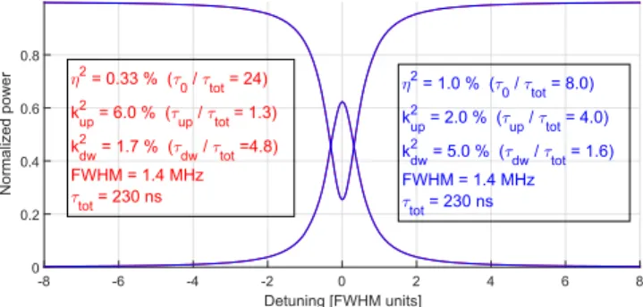
The resonances are identical to each other, presenting a quasi-Lorentzian shape, and are separated by the free spectral range FSR=1 trnd. Figure2shows the resonance proﬁle of a ﬁber

ring resonator similar to the one studied in section 3, assuming fup =fdw=0 and setting kup, kdown and η to

typical values for this kind of resonator. Instead of ν, we adopted the normalized detuning from resonance x=(ν−ν0)/FWHM as the abscissa, where FWHM is the

full width half maximum of the proﬁles and ν0is the

reso-nance frequency. From (7) and (8), we can obtain the

ana-lytical expression for the FWHM as shown in(15).

Since the resonances are identical and the data analysis focuses on the study of the resonance shape, it is common to recast(7) and (8) in a different form through a Taylor expansion

around a resonance frequencyν0, assuming small intrinsic losses

and small coupling losses (η2= 1, k∣ up∣2 1, k∣ down∣2 1).

By doing so, we obtain the following expressions

s 4 4 9 tra 1 1 1 2 2 02 1 1 1 2 2 02 up down 0 up down 0 p n n p n n = - - + -+ + + -t t t t t t

(

)

(

)

( ) ( ) ( ) s 4 , 10 drp 4 1 1 1 2 2 0 2 up down up down 0 p n n = + + + -t -t t t t

(

)

( ) ( )

where the lifetimesτ0,t andup tdown are deﬁned as

Figure 2.Plots of straand sdrpversus x=(ν−ν0)/FWHM with

parameter values typical for afiber ring resonator. The two parameter sets chosen for thisfigure highlight the limits of stationary regime measurements: in fact, the two sets, albeit different, produce perfectly overlapping profiles, making impossible to distinguish between them. In this plot, the blue curves are in the foreground and hide the red ones.

(5)

2 11 0 rnd₂ t t h = ( ) k 2 12 up rnd up2 t = t ∣ ∣ ( ) k 2 . 13 down rnd down2 t = t ∣ ∣ ( )

Physically, the intrinsic lifetimeτ0is the average time that

one photon spends inside the resonator before being lost due to intrinsic losses;t andup tdown, instead, quantify the average time

inside the resonator before being moved to the up-waveguide or the down-waveguide, respectively. To mathematically describe the add-drop system, it is possible to equivalently use the triplet

k k

, ,

2

up2 down2

h

( ∣ ∣ ∣ ∣ ) or the triplet(t t0, up,tdown), since they are

related through equations(11)–(13).

Additionally, we can deﬁne a total lifetime t to taketot

into account all the loss mechanisms by combining the pre-vious lifetimes: 1 1 1 . 14 tot 0 up down 1 t t t t = + + -⎛ ⎝ ⎜ ⎞ ⎠ ⎟ ( )

The functions stra and sdrp (equations (9) and (10)) show

symmetry under the exchange of the lifetimes: for the transfer channel, we notice the exchange symmetry t0«tdown and

1 tup«1 t0+1 tdown, while for the drop channel, we notice

the exchange symmetry tup«tdown. As a practical

con-sequence, these symmetries lead to the possibility for different parameter sets to have identical transfer and drop proﬁles, leading to an ambiguous estimation of the parameters.

In the end, with a slow scan, we cannot unambiguously assign the parameter set (t t0, up,tdown) and we can only

access limited information regarding the main parameters of a resonator, like the FWHM, theﬁnesse  , the quality factor

Qtot, the cavity build-up factor Cband the drop efﬁciency D,

which is the maximum power ratio transmitted to the drop channel. The expressions of these parameters are deduced through the analytical formulas for transfer and drop proﬁles, shown in equations(7)–(10): T T FWHM 1 1 1 15 rnd 2 tot pt p t = ( - ) = ( ) T T FSR FWHM 1 2 16 tot rnd  p pt t = = - = ( ) ( ) Q FWHM 17 tot 0 0 tot n _{pn t} = = ( ) C s k T max 1 18 b cav up2 2 = = -( ) ∣ ∣ ( ) ( ) D s k k T max 1 19 drp up2 down2 2 a = = -( ) ∣ ∣ ∣ ∣ ( ) ( )

From data ﬁtting, we can only deduce the total lifetime

tot

t , since this parameter is symmetric with respect to all three

τʼs, and we can only compute  , Qtotand FWHM. The cavity

build up factor Cb, which is a key value in non-linear optics

applications, remains unknown. To achieve a complete characterisation of the resonator, we have to study the CRD regime.

2.2. CRD profiles

The theory describing the dynamic regime, or CRD regime, is formulated in the time domain and is based on the coupled mode theory described in [30] and extended in [25], which

focuses on the energy exchange between the resonator and the waveguides. We use the complex amplitudes u(t), g t_tra( ) and

g_drp( ) to describe the optical energy stored inside the reso-t

nator mode(equal to u t_{∣ ( )∣}2_{) and the optical powers ﬂowing}

in the waveguides during the fast frequency scan (equal to

g_tra t 2

∣ ( )∣ and g_∣ _drp_{( )∣}t 2_).

The differential equations based on the coupled mode theory, describing an add-drop system when no add wave is injected, are: u t j u t g t d d 1 2 20 0 tot up in w t t =⎛ - + ⎝ ⎜ ⎞_⎠⎟ ( ) ( ) ( ) gtra gin 2 u t 21 up t = - + ( ) ( ) gdrp 2 u t . 22 down t = ( ) ( )

To solve equations (20)–(22), we ﬁx the analytical

structure of the source term g_in( ) as follows:t g t g ej t with t t t,

in( )= 0 f( ) f( )=w( )

wheref(t) is the phase of the laser wave and g_{∣ ∣ is its optical}₀2

power. Since we assume a constant scanning speed Vs and a

non-resonant initial frequency n , we can writei ω(t) and the

instantaneous laser frequency ν(t) as follows [25]:

t V t t t V t 2 2 1 2 d d , 23 i s i s w p n n p f _n = + = = + ⎜ ⎟ ⎛ ⎝ ⎞⎠ ( ) ( ) ( )

obtaining in the end the following expression for g_in( ):t gin( )t =g0exp( (j 2p nit+pV ts 2)).

With a source term of this form, equation (20) can be

integrated using an harmonic oscillator model for u(t), which leads to the following solution[25]:

u t g j t t f t f j 2 exp 0 1 1 up 0 0 tot i tot t w t dw t = -´ - + + ⎛ ⎝ ⎜ ⎞ ⎠ ⎟ ⎡ ⎣ ⎢ ⎤_⎦⎥ ( ) ( ) ( )

where the function f(t) is an auxiliary function deﬁned through the complex error function erf(z):

(6)

f t j W j j W j W t jW 2 exp 2 erf 2 . s i tot 2 s tot i s s p dw t t dw = - - -´ - -⎛ ⎝ ⎜ ⎞_⎠⎟ ⎛ ⎝ ⎜ ⎜ ⎞ ⎠ ⎟ ⎟ ( ) ( )

In both equations, we deﬁne the initial detuning from resonance asni-n0=dni, its angular counterpart asdwi=2p n( i-n0)

and the angular scanning speed as Ws=2pVs.

We can now compute the normalized power proﬁles

stra= ∣gtra g0∣ and s2 drp= ∣gdrp g0∣ substituting u2 (t) into (21)

and(22): s t j t W t f t f j exp 2 2 e 0 1 1 24 t tra i s 2 up i tot 2 tot dw t dw t = - + + ´ - + + t -⎛ ⎝ ⎜ ⎛_⎝⎜ ⎞ ⎠ ⎟⎞ ⎠ ⎟ ⎛ ⎝ ⎜ ⎞ ⎠ ⎟ ( ) ( ) ( ) ( ) s t f t f j 4 e 0 1 1 . 25 t drp down up i tot 2 tot t t dw t = ´ - + + t -⎛ ⎝ ⎜ ⎞ ⎠ ⎟ ( ) ( ) ( ) ( )

Typical examples of stra and sdrp proﬁles are reported in

ﬁgure 3, where we adopted normalized time units for the abscissa(x=t ttot), instead of the absolute time t. Also, the

figure shows the key feature of the dynamic regime, which is the possibility to distinguish between different parameter sets producing identical stationary profiles (the common stationary profile is the one reported in figure 2).

By simultaneously recording the transfer and the drop signals, and thenﬁtting these data with the functions reported

in(24) and (25), it is possible to uniquely obtain the lifetimes

τ0,t andup tdown, completely characterising the system with

one set of measurements. Thefitting procedure is divided into two steps:firstly, we fit the transfer signal to obtain the value oft , which appears in sup train a non-symmetric way under the

exchange with τ0 and tdown; then, while locking t to theup

value resulting from the first fit, we perform a second fit on the drop channel to determine the values ofτ0andtdown, since

they appear in a non-symmetric way in sdrp.

From the three lifetimesτ0,t andup tdown, it is possible to

deduceα, kup and kdown by inversion of equations(11)–(13),

and it is also possible to compute the parameters listed in equations (15)–(19). In addition, it is possible to compute

three auxiliary quality factors Q0, Qup and Qdown, associated

with the intrinsic losses, the up-coupling losses and the down-coupling losses, respectively, deﬁned as in [30]:

Q0=p n t0 0 (26)

Qup=p n t0 up (27)

Qdown=p n t0 down, (28) whereν0is the frequency of the resonance.

3. Experiment onﬁber ring resonator

In this section, we validate the theoretical model of section2

through an experiment on aﬁber ring resonator.

3.1. Setup description and data acquisition

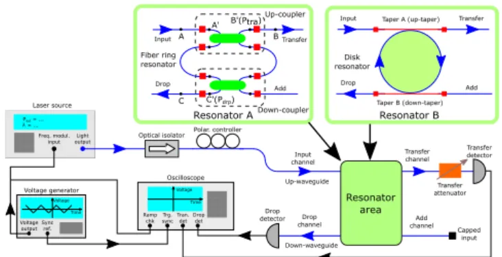
The experimental setup shown infigure 4 was designed to be versatile, allowing the characterisation of both a fiber ring resonator (resonator A) or a WGM resonator using tapered fibers as coupling elements (resonator B). In this section, we are interested in thefiber ring resonator, which was made by spli-cing a pair of 2-by-2 fiber couplers with fibers having a core index n=1.47 and total length L=3.52 m, giving a round trip timetrnd»17 ns and a free spectral range FSR≈58 MHz.

Before the experiment, we characterised the two couplers (labelled as up-coupler and down-coupler in ﬁgure4) in an open

loop conﬁguration by measuring their coupling constant k_{∣ ∣ and}2

their intrinsic losses (commonly called excess losses) using an

Figure 4.Sketch of the setup used to study theﬁber ring resonator (resonator A, section3) and the WGM resonator (resonator B, section4).

Figure 3.Cavity ringdown profiles corresponding to the same parameter sets offigure2, which produce identical stationary profiles. In this regime, the profiles are easily distinguishable.

(7)

infrared power meter (Ando AQ2742). These measurements confirmed the manufacturer specifications, giving k∣ up∣2 »5% and k∣ down∣2 »1%. Also, to take into account the excess losses, we modelled the real coupler as shown infigure 4, using the combination of an ideal coupler(green ellipsis) and four iden-tical lossy elements(red squares) with a transmission factor γ. The values ofg »_up 99%andg_down»98%have been deduced from the measured intrinsic losses.

The resonator was excited by a CW infrared laser source (NetTest Tunics) working in the spectral range from 1500 nm to 1640 nm with a reported linewidth of 150 KHz, and using a modified Littman-Metcalf configuration to achieve a fine wavelength selection through a voltage function generator. In our case, we applied a triangular shaped ramp, which allowed us to cover a spectral interval close to 3 GHz(≈25 pm). After the laser source, we placed an optical isolator and a polarisation controller. In fact, due to mechanical stress inside thefiber ring, the resonance frequenciesν_ℓof the two polarisation families did not coincide, producing a splitting between the two families. Apart from this frequency shift, TE and TM resonances exhibited the same profiles and were not distinguishable.

The two output lines of the ring, which defined the transfer channel and drop channel, were connected to two fast ampli-fied InGaAs detectors (Thorlabs PDA8GS, bandwidth: 9.5 GHz, maximum power: 1 mW), while the second input line, defining the add channel, was not used. An attenuator with an attenuation factor atra protects the detector on the transfer

channel. The signals from the detectors were collected with a digital oscilloscope(Tektronix DPO 7104, bandwidth: 1 GHz). To compare the experimental data with the theory developed in section2, it is necessary to deduce a normalized power proﬁle for both transfer and drop channels, starting from the recorded data. In particular, we want to estimate the normalized power at points B′ and C′ of ﬁgure4, which are the actual output signals of the add-drop resonator.

We start by converting the voltage traces Vtraand Vdrpinto

the detected power traces Pdet,tra and Pdet,drp applying the

calibration lines of the detectors

P V q

m ,

=

-where m and q are the sensitivity(in mV/μW) and the offset (in mV), respectively. Then, taking into account the attenuation factor atraand the excess losses of the couplers, it

is possible to deduce the power proﬁles Ptra(equal to PB¢) and

Pdrp(equal to PC¢): P t P t a V t q m a P t P t V t q m 1 1 ,

tra det,tra tra up tra tra tra tra up drp det,drp down drp drp drp down g g g g = = -= = -( ) ( ) ( ) ( ) ( ) ( )

where t stands for the acquisition times. The last step consists in the normalisation of Ptra and Pdrpto the input power of the

ring Pin, which is marked as PA¢ in ﬁgure4. This input power

is deduced by noticing that, for highﬁnesse resonators, we can compute Pin as the mean value of Ptra when the laser is

off-resonance.

In the end, the normalized power proﬁles ntraand ndrpare

computed as n t P t P 29 tra tra in = ( ) ( ) ( ) n t P t P . 30 drp drp in = ( ) ( ) ( )

These curves are the experimental counterparts of the func-tions stra and sdrpdeduced by the theory of section2and can

be used to characterise the resonator through the data ﬁtting method described in the following subsections.

3.2. Stationary analysis

Because of the exchange symmetry described in section 2.1, stationary proﬁles cannot be used to deduce the single τʼs, but can be used to deuced the total lifetimet .tot

To evaluatet , we perform a least-squarestot ﬁtting on the

experimental proﬁles and then computet via (tot 14). To do so,

we start by replacing ν in (9) and (10) with ν(t) from (23),

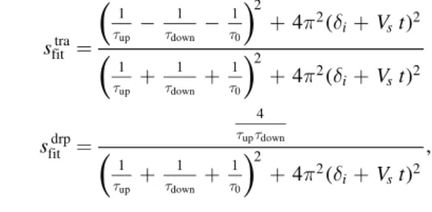
obtaining two functions sfittra and sfit

drp _{depending on the}

vari-ables t;( tup,tdown,t d0, i): s V t V t s V t 4 4 4 , i s i s i s fittra 1 1 1 2 ₂ ₂ 1 1 1 2 ₂ ₂ fit drp 4 1 1 1 2 ₂ ₂ up down 0 up down 0 up down up down 0 p d p d p d = - - + + + + + + = + + + + t t t t t t t t t t t

(

)

(

)

(

)

( ) ( ) ( )

where di=ni-n0 is again the initial detuning from

resonance.

We then deﬁne the sum of the squared residuals RSD as

s t n t RSD ; , , , , 31 n N n n 1

fit up down 0 i exp 2

å

t t t d

=

-=

( ( ) ( )) ( )

where tnis the sampling times of the oscilloscope and nexp( )tn

is the normalized experimental proﬁle deduced through (29)

and (30). By adjusting the parameter set (tup,tdown,t d0, i)

through the MATLAB®ʼs function fminsearch, we can

mini-mize RSD, which quantifies the difference between the theoretical profile and the experimental profile, and obtain the parameter set that better reproduces the data. From the τ values of this set, we compute ttot via (14). The scanning

speed Vs(see (23)) is kept locked during the minimisation of

RSD, its value being assigned as FSR/δt, where δt is the time interval needed to cross one FSR.

Figure5shows the results of the describedﬁtting procedure when applied to a transfer signal and to a drop signal: it is worth noticing that the analysis is performed independently on the two channels, therefore the twot estimates are independent.tot

By repeating the ﬁtting procedure on a series of reso-nances and treating statistically the resultingttotʼs, we obtain a

ﬁnal estimate in the formttot=tˆ stˆ, where

32 i N i tot

å

t= t ˆ ( )

(8)

N 1 33 i N i 2

å

s = t -t -tˆ (ˆ ) ( )

with ti_tot being the values resulting from data ﬁtting and N being the number of analysed resonances (in our case N=13). The dispersion of thetitotvalues can be caused by a

combination of electric noise of the detectors and power instability of the laser source: in fact, both effects can affect the experimental proﬁles in an unpredictable way and produce shapes that yield different results under our analysis.

Finally, it is possible to switch the roles of the up-coupler and the down-coupler (‘inverted conﬁguration’) and repeat the entire procedure to obtain two other independent estimates fort , reaching the total of four independent estimates, astot

reported in table1.

3.3. Cavity ringdown analysis

In the case of CRD proﬁles, we propose an original analysis that uses transfer and drop proﬁles together to estimate the three lifetimesτ0,t andup tdown.

Initially, we focus on the transfer proﬁle and deﬁne the quantityRSDtra as:

s t V n t RSD ; , , , , n N n n tra 1

tra s i 0 up down tra 2

å

d t t t

=

-=

( ( ) ( ))

where stra is the theoretical proﬁle (24) and ntra is the

nor-malized experimental proﬁle (see (29)) and tn are again the

sampling times of the oscilloscope.

As for the stationary case, by minimisation of RSDtrawe

can determine parameter set that better reproduces the data: in this case the adjusted parameters are the scanning speed Vs,

the initial detuning d , the intrinsic lifetimei τ0and the

cou-pling lifetimest andup tdown. At the end of the minimisation

procedure, however, only Vs,d andi t are correctly estimated,up

while τ0 and tdown cannot be deemed trustful due to the

exchange symmetry discussed in section 2.2.

To getτ0andtdown, we need to analyse the drop proﬁle,

because these parameters appear in a non-symmetric way in (25) and the minimization algorithm can resolve their values.

Therefore, we deﬁne RSDdrpas:

s t V n t RSD ; , , , , n N n n drp 1 drp s i up lock 0 down drp 2

å

d t t t = -= ( ( { } ) ( ))

and minimize its value by adjusting only the values ofτ0and

down

t , while keeping d , Vi s and tup locked to the values

obtained from theﬁrst minimisation.

In the end, the values of d , Vi s and t from the ﬁrstup

minimisation and the values oft and0 tdown from the second

minimisation are our estimates for the entire parameter set

V ,s d t ti, 0, up,tdown

( ). Figure6shows the typical results of the entire analysis procedure, having the ﬁtting curves obtained through fminsearch in red and the normalized power proﬁles in blue.

As an additional veriﬁcation of the consistency of the parameter set obtained through the two-step minimisation, we plot an additional green transfer curve (s_trachk) using these values and re-compute the residuals with respect to the experimental ntra (RSDchk), ﬁnding that the green curve is

very close to the red curve and that the residualsRSDchk are

almost identical to the residualsRSDtra.

By ﬁtting a number of resonances, we can give a ﬁnal estimate in the form t=tˆ stˆ for each lifetime, following

the same statistical method described in the previous section (see (33), N=17 in this case). Then, from these estimates,

we can computet (see (tot 14)) and deduce the values of k∣ up∣2

and k∣ down∣ by inverting equations2 (11)–(13) and recalling

thattrnd=17 ns.

The dispersion of τʼs values can be related to the same effects we discussed during the stationary analysis, i.e. elec-tric noise of the detectors and powerﬂuctuations of the laser source, but also to the mathematical complexity of theﬁtting functions (24) and (25). In fact, due to this complexity, it is

possible that fminsearch could converge in a region of relative minima close to the absolute minimum associated with the expected values. The evaluation of the contribution of each of these error sources to the τʼs dispersion is a difﬁcult task, therefore we treated the results with the statistical method described before, which estimates the overall dispersion.

Figure 5.Typical dataﬁtting results obtained through the

minimisation of RSD. The red curves are theﬁtting proﬁles s_fittra_and

s_fitdrp, while the blue curves are the normalized experimental proﬁles ntraand ndrpfrom(29) and (30).

Table 1.Stationary regime results for thefiber ring resonator. Configuration and analysed profile ttot=tˆ stˆ ( )ns

Direct transfer 116±6

Direct drop 119±12

Inverted transfer 118±7

(9)

As in section3.2, we performed measurements in direct and inverted configurations: all results are shown in table2. It is worth mentioning that, while comparing the results of the two configurations, the roles of the two couplers are exchanged and an up-parameter in one configuration has to be compared with the corresponding down-parameter in the other.

In the end, the presented analysis is able to reproduce the values of kup and kdown found during the coupler

character-isation, as well as to give t estimates consistent with thetot

ones deduced from stationary measurement(see table1): this

means that our procedure is reliable and can be used to characterise an unknown resonator. We also notice that the characteristic lifetimes are determined with an accuracy that ranges from 3% to 8%.

4. Experiment with a WGM resonator

The analysis technique developed for theﬁber ring resonator can be used to study the coupling of two taperedﬁbers with a high Q home-made WGM disk resonator. The resonator was fabricated in MgF2(n=1.37) with the technique described in

[31] and has a diameter dr=3.83 mm. This kind of study

allows to deduce intrinsic properties of the resonator(like τ0,

η2

and Q0), as well as determining the strength of the coupling

through k∣ up∣ and k2 ∣ down∣ : the knowledge of these parameters2

is extremely important when the WGM resonator is used in applications like sensing orﬁltering, or in basic studies like in theﬁeld of non-linear optics.

4.1. Setup description and data acquisition

For this experiment, we again used the setup shown inﬁgure4, with the resonator being the WGM crystalline disk(resonator B). In this case, light was coupled to the resonator through two home-made biconical taperedﬁbers [31], commonly addressed as tapers

(red lines in ﬁgure4). To move the two tapers and couple them to

the disk, we used two independent translational stages with submicrometrical resolution along the three directions, while keeping the disk in aﬁxed position through an holder.

Positioning the biconical tapers was a critical part of the experiment in order tofind the optimal configuration, as sketched infigure7. While keeping the tapers in contact with the disk, we moved the up-taper from left to right in the disk equatorial plane and observed the transfer signal during a slow frequency scan, allowing us tofind the region with the proper diameter to achieve good coupling(zone 2 in figure7). From our estimates, zone 2

had a diameter around 4μm and the taper was thick enough to assume no losses between zone 1 and zone 2 and we could assume PA=PA¢. However, to the right of zone 2, losses could

be present due to the diameter reduction: we could take them into account by measuring the powers PBand PAthrough an infrared

power meter (Ando AQ2742) and deﬁning the up-taper trans-mission factor g =_up PB PA¢=PB PA (typically g »up 90%).

The entire procedure was then repeated to align the down-taper by putting the laser source on the drop channel and the drop detector on the add channel.

After both tapers had been aligned as shown inﬁgure7, the oscilloscope recorded, during a slow frequency scan, a series of dips for the transfer channel and a series of spikes for the drop channel. Differently from theﬁber ring, we observed several different resonances (instead of the repetition of an identical one) and this is because the disk supports a great number of WGMs in the observed spectral interval (≈3 GHz), each characterised with its own resonant

Figure 6.Typical results of thefitting procedure described in the main text. The red curves are the profiles obtained after the minimisation of RSDtraand RSDdrp, while the green profile is the

consistency plot(s_trachk_).

Table 2.CRD regime results for theﬁber ring resonator. Direct conf. Inverted conf. ns tot t ( ) 120±5 124±4 kup2 % ∣ ∣ ( ) 4.99±0.16 0.96±0.06 kdown2 % ∣ ∣ ( ) 1.16±0.16 4.9±0.3

Figure 7.Relative position of the tapers and the disk after alignment: we marked with dashed lines the two coupling zones described in the main text. Theﬁgure is not intended to be in scale and the details are exaggerated for the sake of clarity.

(10)

frequency, its own k( up,kdown) set and its own quality factor

Qtot[28].

Once we selected the resonance to study, we maximized its contrast using the polarisation controller and then increased the scanning speed Vs, switching to the CRD

regime. The acquired CRD proﬁles undergo the same nor-malisation procedure described in section 3.1 and therefore we have P P P a V q m P P P V q m n P P n P P and , tra A B up

tra det,tra tra tra up drp C C det,drp drp drp tra tra in drp drp in g g = = = -= = = -= = ¢ ¢ ( ) ( )

where Pinis again the out-of-resonance optical power deduced

by the power signal Ptra. 4.2. Data analysis

From the normalized proﬁles, it is possible to deduce the lifetimest ,uptdownandτ0using theﬁtting procedure validated

in section3on thefiber ring resonator. As previously noted, for the disk resonator each resonance is physically different, corresponding to one of the several WGMs that can be excited and being characterised by its own set of parameters: figure8shows the results for two typical resonances, labelled as A(left side) and B (right side). Similarly to the case of the fiber ring resonator, the figure reports the normalized exper-imental profile in blue, the fitting curve in red and the con-sistency curve in green: the two resonances are obtained for different scanning speeds and coupling conditions.

Since the observed spectral window was less than the disk FSR(≈18 GHz), we cannot analyse replicas of A and B to deduce the experimental error with the statistical method seen in section 3(see (33)) and we cannot estimate directly

the errors on the τʼs and the other parameters of the WGM resonator. Therefore, in reporting these quantities in table 3, we decide to round the numbers to two signiﬁcant digits, in analogy with table2.

Even if the disk resonances appear similar to the ones of the ﬁber ring resonator, the values of the parameters are very different. In fact, the intrinsic losses (η2) and the coupling losses( k∣ up∣ and k2 ∣ down∣2) have a magnitude of 10−5

or 10−6, meaning that very little light is lost by or coupled into the resonator. The Qʼs have very high values, typically around 108 and 109, with the intrinsic quality factors Q0ʼs

close to the state-of-the-art values.

However, for practical applications like sensing and non linear optics studies, the most important parameter is the ﬁnesse  , which is a measure of the average number of round trip performed by a photon inside the resonator before being lost.

Together with the finesse  , it is usual to define the intrinsic finesse  , which takes into account only the0

intrinsic losses, just as the intrinsic quality factor Q0:

Q FSR, 34 0 0 rnd 0 0  p t t n = = ( )

whereν0is the resonance frequency. The intrinsicﬁnesse0

is reported in table 3 along with the other parameters. In particular, for resonance B we have obtained the highest values of Q0 =7.5·108and =0 7.2·104.

Since the two resonances A and B correspond to different WGMs, we expect the modes to have different geometries,

Figure 8.Transfer and drop profiles for two typical CRD resonances (A on the left and B on the right). The figure reports the normalized experimental profile in blue, the fitting curve in the red and the consistency curve in the green; it also shows the τʼs values, while the complete numerical results are listed in table3. The two resonances are obtained for different scanning speeds and coupling conditions.

(11)

producing different coupling factors k∣ up∣ and k2 ∣ down∣ : this is2

conﬁrmed by the numerical results of table 3. The small difference inη2and τ0can be explained by the difference in

the mode geometry and taking into account the fact that the intrinsic losses are mostly due to surface imperfections. In fact, since the two modes touch the surface in different points with their evanescent tails and the resonator surface is not perfectly homogeneous, the surface losses for the two modes can be slightly different.

5. Conclusions

In this work, we have studied a ring resonator in the add-drop conﬁguration, which is a common conﬁguration in applied optics as well as in some fundamental studies involving high-Q WGM resonators. In all these cases, the deduction of the intrinsic properties of the resonator and its interaction with the coupling waveguides is a fundamental aspect.

The standard analysis method, which is based on the data fitting of stationary profiles, proved to be not sufficient for this purpose, and therefore we investigated a different approach, studying the CRD regime, which allowed us to fully characterise the system. We developed a theoretical model describing both the transfer and drop signals, starting from the known solution of the single coupler case found in literature, and then set up the experiment to check the validity of the model.

The theoretical model predicted well the experimental CRD profiles for both transfer and drop channels and we developed an original fitting procedure to deduce the para-meters characterising the resonator. The analysis method was tested with an experiment on afiber ring resonator of known characteristics. The expected values were well reproduced and the error on these estimates, deduced by a statistical analysis, were equal to a few percentage points.

The validated analysis method, which was developed to be general and independent from the speciﬁc type of

resonator, was then used to characterise a high Q WGM disk resonator. From a simultaneous acquisition of the transfer and drop signals, we could assess the main parameters of the resonator and its coupling to the waveguides, achieving the main goal of this work.

We also envisage an addition to the theoretical model developed in this work, so that it can take into account the possibility of selective ampliﬁcation (negative lifetime τ0

[32]) and coupling between two resonators [33].

Acknowledgments

We thank Professor Duccio Fanelli from the University of Florence, Italy, for useful discussions and Mr Franco Cosi from IFAC-CNR for manufacturing the MgF2disk.

This research study was partially supported by Ente Cassa di Risparmio di Firenze project No. 2014.0770A2202.8861. S Berneschi acknowledges the European Community for its funding within the framework of the projects Hemospec (FP7-611682). G Frigenti and S Soria acknowledge funding from the bilateral CNR-CONACYT project‘All optical morphogenesis of nanostructures characterized by photo acoustic microscopy’ (2017–2019). ORCID iDs G Frigenti https://orcid.org/0000-0002-4290-3158 M Arjmand https://orcid.org/0000-0001-9993-4767 Y Dumeige https://orcid.org/0000-0001-9003-0809 References

[1] Chiasera A, Dumeige Y, Féron P, Ferrari M, Jestin Y, Conti G N, Pelli S, Soria S and Righini G 2010 Laser Photonics Rev.4 457

[2] Guo H, Karpov M, Lucas E, Kordts A, Pfeiffer M H P, Brasch V, Lihachev G, Lobanov V E, Gorodetsky M L and Kippenberg T J 2017 Nat. Phys.13 94

[3] Liang W, Eliyahu D, Ilchenko V S, Savchenkov A A, Matsko A B, Seidel D and Maleki L 2015 Nat. Commun. 6 7957

[4] Wang C Y, Herr T, Del’Haye P, Schliesser A, Hofer J, Holzwarth R, Hänsch T W, Picqué N and Kippenberg T J 2013 Nat. Commun.4 1345

[5] Kippenberg T J, Holzwarth R and Diddams S A 2011 Science 332 555

[6] Farnesi D, Barucci A, Righini G, Berneschi S, Soria S and Conti G N 2014 Phys. Rev. Lett.112 093901

[7] Farnesi D, Barucci A, Righini G, Conti G N and Soria S 2015 Opt. Lett.40 4508

[8] Farnesi D, Righini G, Conti G N and Soria S 2017 Sci. Rep.7 44198

[9] Farnesi D, Berneschi S, Cosi F, Righini G C, Soria S and Conti G N 2016 J. Vis. Exp.110 e53938

[10] de Cumis M S et al 2016 Laser Photon Rev.10 153 Table 3.Analysis results for the WGM resonances‘A’ and ‘B’ from

ﬁgure8. Resonance A Resonance B τ0 (ns) 1000 1300 ns up t ( ) 1800 15000 ns down t ( ) 4400 3000 ns tot t ( ) 580 840 η2 10 10_· -5 _{8.8 10}_· -5 kup2 ∣ ∣ 6.0 10_· -5 _{0.73 10}_· -5 kdown2 ∣ ∣ 2.5 10_· -5 _{3.6 10}_· -5 Q0 6.3 10· 8 7.5 10· 8 Qup 11 10· 8 91 10· 8 Qdown 26 10· 8 18 10· 8 Qtot 3.5 10· 8 5.0 10· 8  3.3 10_· 4 _{4.8 10}_· 4 0  6.0 10_· 4 _{7.2 10}_· 4

(12)

[11] Fescenko I, Alnis J, Schliesser A, Wang C Y,

Kippenberg T J and Hänsch T W 2012 Opt. Express20 19185

[12] Liang W, Ilchenko V S, Savchenkov A A, Matsko A B, Seidel D and Maleki L 2010 Opt. Lett.35 2822

[13] Peccianti M, Pasquazi A, Park Y, Little B, Chu S, Moss D and Morandotti R 2012 Nat. Commun.3 765

[14] Ristic D et al 2016 J. Lumin.170 755

[15] Yao X S and Maleki L 1996 J. Opt. Soc. Am. B13 1725 [16] Liang W, Eliyahu D, Ilchenko V S, Savchenkov A A,

Matsko A B, Seidel D and Maleki L 2015 Nat. Commun. 6 7957

[17] Moniﬁ F, Friedlein J, Özmedir Ş K and Yang L 2012 J. Lightwave Technol.30 3306

[18] Razdolskiy I, Berneschi S, Conti G N, Pelli S, Murzina T V, Righini G C and Soria S 2011 Opt. Express19 9523 [19] Roy S, Prasad M, Topolancik J and Vollmer F 2010 J. Appl.

Phys.107 053115

[20] Poellinger M and Rauschenbeutel A 2010 Opt. Express18 17764

[21] Razdolskiy I, Berneschi S, Conti G N, Pelli S, Murzina T V, Righini G C and Soria S 2011 Opt. Express19 9523

[22] Yang Y, Madugani R, Kasumie S, Ward J M and Chormaic S N 2016 Appl. Phys. B122 291

[23] Giorgini A, Avino S, Malara P, Natale P D and Gagliardi G 2017 Sci. Rep.7 41997

[24] Chen L, Liu Q, Zhang W G and Chou K C 2016 Sci. Rep.6 38922 [25] Dumeige Y, Trebaol S, Ghişa L, Nguyên T, Tavernier H and

Féron P 2008 J. Opt. Soc. Am. B25 2073

[26] Gorodetsky M L and Ilchenko V S 1999 J. Opt. Soc. Am. B 16 147

[27] Yariv A 2000 Electron. Lett.36 321

[28] Little B E, Laine J P and Haus H A 1999 J. Lightwave Technol. 17 704

[29] Matsko A and Ilchenko V 2006 IEEE J. Sel. Top. Quantum Electron.12 3

[30] Haus H A 1984 Waves and Fields in Optoelectronics (Englewood Cliffs, NJ: Prentice-Hall) ch 7

[31] Merrer P H, Saleh K, Llopis O, Berneschi S, Cosi F and Conti G N 2012 Appl. Opt.51 4742

[32] Rasoloniaina A, Huet V, Nguyên T K N, Cren E L, Mortier M, Michely L, Dumeige Y and Féron P 2014 Sci. Rep.4 4023 [33] Rasoloniaina A, Huet V, Thual M, Balac S, Féron P and