Analysis of the influences of uncertainties in input variables on the outcomes of the Heliosat-2 method

HAL Id: hal-00465617

https://hal-mines-paristech.archives-ouvertes.fr/hal-00465617

HAL is a multi-disciplinary open access archive for the deposit and dissemination of sci-entific research documents, whether they are pub-lished or not. The documents may come from teaching and research institutions in France or abroad, or from public or private research centers.

L’archive ouverte pluridisciplinaire HAL, est destinée au dépôt et à la diffusion de documents scientifiques de niveau recherche, publiés ou non, émanant des établissements d’enseignement et de recherche français ou étrangers, des laboratoires publics ou privés.

Analysis of the influences of uncertainties in input

variables on the outcomes of the Heliosat-2 method

Bella Espinar, Lourdes Ramirez, Jesus Polo, Luis Zarzalejo, Lucien Wald

To cite this version:

Bella Espinar, Lourdes Ramirez, Jesus Polo, Luis Zarzalejo, Lucien Wald. Analysis of the influences of uncertainties in input variables on the outcomes of the Heliosat-2 method. Solar Energy, Elsevier, 2009, 83, pp.1731-1741. �10.1016/j.solener.2009.06.010�. �hal-00465617�

Espinar, B., Ramírez, L., Polo, J., Zarzalejo, L.F., Wald, L., Analysis of the influences of uncertainties in input variables on the outcomes of the Heliosat-2 method. Solar Energy, 83, 1731-1741, 2009.

doi:10.1016/j.solener.2009.06.010

ANALYSIS OF THE INFLUENCES OF UNCERTAINTIES IN INPUT

VARIABLES ON THE OUTCOMES OF THE HELIOSAT-2 METHOD

Espinar, B.1_{, Ramírez, L.} 1_{, Polo, J.}* 1_{, Zarzalejo, L.F.} 1_{, Wald, L.} 2 1 _{Solar Platform of Almería (Energy Department, CIEMAT), Ctra. Senés s/n,}

04200 Tabernas (Almería), Spain.

2 _{Centre Energétique et Procédés, Mines ParisTech,} BP 207, 06904, Sophia Antipolis cedex, France.

Abstract

The Heliosat-2 method, which employs satellite images to assess solar irradiance at ground level, is one of the most accurate among the available operational methods. Its input variables have uncertainties which impact on the final result. The General Law of Uncertainty Propagation is employed to analyze the impact of these uncertainties on a single pixel with Meteosat-7 inputs in various stages, beginning with the sensitivity coefficients and the changes induced in the clear-sky index (KC) by each independent

variable. Once these coefficients are known, the partial combined standard uncertainty (CSU) is calculated for KC from each independent variable and albedo. Finally, the total CSU of KC is calculated.

All of the results are in agreement and show that the most influential variables in the uncertainty of estimation of cloudy skies are, in this order, the Linke turbidity factor (54% of KC value), terrain elevation

(33%), the calibration coefficient of the satellite sensor (13%) and the ground albedo (5%). What causes the initial uncertainty in the ground albedo is its variation over time and the difficulty in assessing it from a reflectance time-series for mixed clear and cloudy skies. The Linke turbidity factor is the most influential variable on the width of the uncertainty interval, not only because of its own uncertainty (17% in this study), but because it is also used in numerous intermediate calculations. For clear skies, the partial CSUs are considerably lower, except for ground albedo (5% also).

Keywords: uncertainty analysis, satellite, solar irradiance, Heliosat

NOMENCLATURE

CC Calibration coefficient of the satellite sensor (W m-2 _sr-1₎ CSU Combined standard uncertainty

DC Digital count

G Global solar irradiance on horizontal surface (W m-2₎

GC Clear-sky global solar irradiance on horizontal surface (W m-2₎

I

KC Clear-sky index (unitless)

L Radiance received by the satellite sensor (W m-2 _sr-1₎

n Cloud index (unitless), this quantity is specific to the Heliosat method SSI Surface solar irradiance

T Atmospheric path transmittance from the Sun to the Earth’s surface (unitless)

Tsat Atmospheric path transmittance from the Earth’s surface to the satellite sensor (unitless)

TL Linke turbidity factor (unitless)

z Elevation of terrain above mean sea level (m)

α Solar elevation angle (rad)

α sat Satellite elevation angle (rad)

ρ * _{Albedo or reflectance observed by the satellite sensor (unitless)}

ρ atm Atmospheric albedo or reflectance (unitless)

ρ ef Effective cloud albedo or reflectance (unitless)

ρ g Ground albedo or reflectance (unitless)

ρ gref Reference ground albedo or reflectance (unitless)

ρ n Albedo or reflectance of very bright clouds; also called cloud albedo (unitless)

ρ α Apparent albedo or reflectance of the Earth’s surface (unitless)

1. Introduction

Solar radiation is one of the best alternative energy sources, since it is permanent, abundant and widely distributed over the face of the Earth (Şen, 2004). Solar radiation is also a required environmental variable in many applications (Zarzalejo, 2006), such as weather prediction, forest fire prevention, calculation of the potential evapotranspiration (Mahmood and Hubbard, 2005; Bois et al. 2008), crop performance (Reuter et al., 2005), and climate change (Speranza et al., 2003), among others.

The superiority of satellite data over interpolation of radiometric network measurements for estimating the surface solar irradiance (SSI) has been demonstrated (Perez et al., 1997; Zelenka et al., 1999). Evaluation of the SSI requires continuous observation due to seasonal and weather variations in radiant flux intensity received on the surface. Geostationary meteorological satellites, which record several images of the same terrestrial zone per hour, provide a very good means of estimating SSI (e.g., Perez et al., 2002 for the GOES satellite; Beyer et al., 1996; Rigollier et al., 2004 for Meteosat). The Heliosat method is one of the most precise methods for estimating SSI from satellite data (Grüter et al., 1986; Raschke et al., 1991). The new version, Heliosat-2, among other advantages, has even higher accuracy (Rigollier et al., 2004), and its use is therefore widespread in the scientific community in many projects involving the use of satellite images to estimate solar radiation, as mentioned by Vera (2005) in his review of recent scientific literature. The software is available on the Internet since 2004 (www.helioclim.net) and has been downloaded more than 2000 times since then.

Heliosat-2 integrates the knowledge gained from experience in using the original Heliosat method. In the former version, various empirical parameters were determined statistically with the aid of simultaneous ground measurements, (Cano et al., 1986; Diabaté et al., 1988, 1989b; Moussu et al., 1989). The current version expresses these parameters using physical laws, making it applicable anywhere on Earth

(Rigollier et al., 2004). These variables are found for all of the pixels in the image and must be known with the least possible uncertainty, since the uncertainty in the method’s results depends on them. In this sense, this uncertainty analysis finds out which variable or variables most influence the total method uncertainty, and must therefore be known a priori with the least uncertainty possible. It also suggests some improvements in the method that would achieve a more accurate assessment of the SSI. This would be very advantageous in solar energy applications where irradiance estimations are often critical in selecting profitable sites, and guaranteeing solar energy projects.

To perform the uncertainty analysis, standard procedure ISO 1995 is employed, tailoring it to the case of the Heliosat-2 method which is described along with its input variables. Once the framework for analysis is laid, the variables are instantiated to produce a numerical example and estimate the influences of the respective input variables on the Heliosat-2 method outputs.

2. Description of the Heliosat-2 method

The Heliosat-2 method is based on the principle that attenuation of the downwelling shortwave radiation by the atmosphere over a pixel is determined by the magnitude of change between the reflectance that should be observed under a very clear sky and that currently observed (Pastre, 1981; Cano et al., 1986; Stuhlmann, et al., 1990). Heliosat-2 is based on the fundamentals of its predecessor, the Heliosat method (Cano et al., 1986; Diabaté et al., 1988, 1989b), that is, the computation of a cloud index n from apparent albedo (ρ α), ground albedo (ρ g), and albedo of very bright clouds (ρ n). The current version of Heliosat

includes such features as (Rigollier et al., 2004) image calibration for any change in the satellite sensor (Lefèvre et al. 2000; Rigollier et al., 2001, 2002), adoption of a clear-sky radiation model (Rigollier et al., 2000), computation of albedo values (ρ α , ρ g and ρ n) (Lefèvre et al., 2002), use of the clear-sky index

(KC) (Beyer el al., 1996), and the relationship between the cloud index n and KC (Rigollier and Wald,

1998).

In Heliosat-2, the global SSI, G, is estimated using KC and the global SSI under clear skies, GC, using the

ratio:

K

=

G

G

(1)

where GC is calculated using the clear-sky model proposed in the most recent version of the European

Solar Radiation Atlas (ESRA, 2000; Rigollier et al., 2000, revised in Geiger et al., 2002). The clear-sky index KC is related to the cloud index, n, by the following parametric expression (Rigollier and Wald,

This uncertainty study concentrates on the linear range, -0.2 ≤ n < 0.8, because it represents most of the cloudy conditions. For each pixel in the image, n is estimated using the apparent albedo ρ α , cloud albedo ρ n and ground albedo ρ g, expressed as:

n=

ρ

−

ρ

ρ

−

ρ

These values are evaluated by using radiance received by the satellite sensor (L) and additional information, such as the calibration coefficient of the sensor itself (CC), the maximum total irradiance

I

the geographic variables that define the pixel of interest: latitude, longitude and terrain elevation. This information is used to estimate the atmospheric contribution by its reflectance (ρ atm) and transmittance

(T) from the Sun to the Earth’s surface and the transmittance (Tsat) from the Earth’s surface to the satellite

sensor. T and Tsat are estimated using the same equations, with the solar elevation angle α for the former

and the satellite elevation angle α sat for the latter. So the apparent albedo of the Earth’s surface (ρ α) is related to the albedo observed by the satellite sensor (ρ ∗_{) by:}

ρ

=



ρ−ρ



T

_

α,T

_

T

_

α

,T

_

and the albedo of very bright clouds (ρ n) is calculated the same way, but using the effective cloud albedo

(ρ ef):

ρ

=



ρ

−

ρ



T

_

α,T

_

T

_

α

,T

_

The ground albedo ρ g is the contribution to ρ α that is attributed exclusively to the Earth’s surface. In principle, its value is the minimum in a series of ρ α, since a low ρ α means absence of clouds in the pixel of interest. There are different possible strategies for selecting ρ g (Rigollier et al., 2004; Lefèvre et

al., 2007), including restrictions for an acceptable threshold and for the maximum permissible change from one image to the next (Cano et al., 1986; Moussu et al., 1989; Lefèvre et al., 2002), which determine the uncertainty intrinsic to ρ g. This strategy is discussed further.

3. Methodology 3.1 General methodology

The General Law of Uncertainty Propagation (ISO, 1995) is used to study the uncertainty in the Heliosat-2 method. The uncertainty of an independent variable xi –also called the standard uncertainty– is denoted

analysis of a series of observations, or it can be estimated by non-statistical methods, such as external information, for example, observer experience. The ISO standard makes a distinction between these two cases in the nomenclature, labeling them “Type A uncertainty” and “Type B uncertainty” respectively. In this analysis, uncertainties of all independent variables are Type B, based on knowledge gained by previous experience. A normal distribution is assumed for all the variables under study.

If the variable y is deduced from N input variables with a functional relationship:

y = f(x1,x2,..xN.)(6)

then the combined standard uncertainty of y (hereafter CSU) is denoted by uc(y)x1,...,xN. The CSU results from combining the uncertainties of these N input variables. For independent variables xi, uc(y)x1,...,xN is

calculated as the following positive square root:

u



y 

=



∑



∂

f

∂

x



u

_

_x



The partial derivative ∂f/∂xi, also called the sensitivity coefficient, describes how much estimated y varies

with changes in input xi (ISO, 1995). Let the change in a variable be denoted by the symbol Δ. In

particular, the change produced in y by a small change in the variable xi, is calculated as



Δy 

=



∂

f

∂

x





Δx



(8)

Note that Equation (8) is the formulation of the former General Law of Error Propagation (ISO 1995, entry E.3.2) which is no longer recommended. If this Δxi is the same as its uncertainty, u(xi), then:



Δy 

i

=



∂

f

∂

x



u  x



(9)

Thus (Δy)xi can be used to calculate uc(y)xi. If variables xi are independent of each other, then the changes

in y are also independent. All partial derivatives are evaluated in the corresponding input variable value and the chain rule of derivatives is applied when needed.

Relative values are also commonly used. The relative change induced in the measurand can be calculated as

Δy / y

u



y 

=

1

y



∑



∂

f

∂

x



u

_

_x

=

1

y



∑



Δy



(10)

In the following, the term partial CSU is understood as the uncertainty caused by one or several independent variables only. If all of them enter in the calculation, then it is the total CSU.

For the clarity of this paper, it should be noted that the term uncertainty is not related to measurement or estimation accuracy, but, by definition of the International vocabulary of basic and general terms in

metrology (ISO 1993, entry 3.9) is “…a parameter associated with the result of a measurement that

characterizes the dispersion of the values that could reasonably be attributed to the measurand”. Therefore, the uncertainty of a variable is not necessarily an indication of the likelihood that the measurement is near the value of the measurand. It is simply an estimate of the likelihood of nearness to the best value that is consistent with presently available knowledge (ISO 1995). This study only explains the uncertainty of the clear-sky index, KC, calculation method. Some characteristics of satellite-retrieved

data, such as different temporal and spatial scales, have to be considered when used instead of ground measurements. In fact, satellite data are instantaneous measurements over a small solid viewing angle, while ground measurements are integrated over time and the solid angle of 2π (Noia et al., 1993). So, the model has an intrinsic uncertainty due to this kind of consideration, which is, however, out of the scope of this study.

In the following sections, the changes induced in KC are calculated using Equation (9), one by one for

each input variable. Since the chain rule of derivatives is applied, it is possible to separate this calculation for each albedo in Equation 3, keeping in mind that ∆ (y)xi is the sum of two contributions, by ρ α and

ρ n in this case. If G and G* respectively, denote the actual and estimated SSI, KC and

K

actual and the estimated value of the clear-sky index, respectively, and ∆ KC is the change induced in KC

when the input variables have changed, then:

G =G

K

=G



K

+ΔK



=G+G

ΔK

Though GC is necessary to calculate G from KC, this study does not deal with ∆ GC as GC is calculated by

a clear-sky model not included to Heliosat-2. Then the change induced in G is deduced from Equation (11) as:

ΔG=G

ΔK

ΔG

G

100=

G

ΔK

G

100=

ΔK

K

100

3.2 Analysis of the uncertainties of Heliosat-2

The independent input variables in the Heliosat-2 are the image digital count (DC), the satellite sensor calibration coefficient (CC) because it changes over time, the solar elevation angle (α ), the satellite elevation angle (α sat), the Linke turbidity factor (TL), the terrain elevation (z) and the ground albedo (ρ g).

From these input variables, Heliosat-2 computes ρ α for each pixel, ρ n, and then estimates n, KC and G.

The aim is to find out the total CSU induced in the estimation of KC and G with this method and which

independent variable most contributes to it. This is found by computing the changes induced in n by the uncertainties in each of the input variables. From Equation (2),

u



K



=u



n 

i

(15) where the negative sign disappears because CSU is always defined as positive, as mentioned above.

Change induced in KC by the uncertainty in apparent albedo ρ α

The apparent albedo is determined as a function of the following variables (Rigollier et al., 2004):

ρ =ρ



CC,DC,α



ρ

=ρ

_

α,α

,T

_

T=T

_

α,T

,z

_

T

=T

_

α

,T

,z

_

K

as



ΔK



=

ΔK



of each of these variables. That is,



ΔK



=−



Δn



=

=−



∂

n

∂

ρ



{



∂

ρ

∂

CC



u



CC







∂

ρ

∂

DC



u



DC







∂

ρ

∂

α



u



α



}









∂

ρ

∂

α



u



α







∂

ρ

∂

T



u



T







∂

ρ

∂

z



u



z





Change induced in KC by the uncertainty in ground albedo ρ g

Under clear skies, ρ g is the same as ρ α because there are no clouds. Then, ρ g can be selected a priori

as the minimum value in a series of ρ α over a given time period. This selection is not as direct, and several strategies have been developed to avoid such shortcomings as having to place a value on defects not detected in the original image or cloud shadows, which create artificially low ground reflectance (Lefèvre et al., 2002; Rigollier et al., 2004; Lefèvre et al., 2007). This study of the Heliosat-2 method selects ρ g as proposed by Lefèvre et al. (2007). As the period covered is limited to one month, there is no

guarantee that this minimum corresponds to a clear-sky situation, but only the clearest sky condition. Once this minimum is found, it is compared to a reference ground albedo, ρ gref taking into account an

interval of maximum acceptable change in ρ g. If the difference between this reference and the candidate

ρ g is larger than this maximum acceptable change interval, then the end of the interval is proposed as the

updated value of ρ g. That is, ρ g is related to ρ α, but is not systematically selected from a ρ α series, which is why ρ g is considered one of the Helisoat-2 independent input variables. As noted above, the

selected strategy for determining ρ g also determines its uncertainty. The change induced in KC by ρ g can



ΔK



=−



Δn



=−



∂

n

∂

ρ



u ρ



Change induced in KC by the uncertainty in cloud albedo ρ n

The cloud albedo is a function of the following variables (Rigollier et al., 2004):

ρ

=ρ



α



ρ

=ρ

_

α,α

,T

_

T=T

_

α,T

,z

_

T

=T

_

α

,T

,z

_

Following the procedure described above, the change



ΔK



calculated by the addition of changes induced by the uncertainty in each of the variables, α , α sat,

T

and z:



ΔK



=−



Δn



=

=−



∂

n

∂

ρ



{



∂

ρ

∂

α



u



α



}







∂

ρ

∂

α



u



α







∂

ρ

∂

T



u



T







∂

ρ

∂

z



u



z





4. Allocation of values to input variables

Once the framework for the uncertainty analysis is laid, variables must be instantiated. Two types of input variables can be distinguished, on the one hand, the inputs which are inherent in the geographical location of site, either because of the time or the image in hand. In this group are site latitude and longitude, α ,

α sat and z. On the other hand, are the random variables, such as the description of the atmosphere through

the digital count, DC, and the Linke turbidity factor, TL; the condition of the satellite sensor through its

updated calibration coefficient, CC; and the reflectance of the Earth’s surface, ρ g. In an attempt to

systematize the estimation method, TL is modeled by adopting a monthly value and interpolating the daily

values (Remund et al., 2003), and then a periodic annual series is used. There is no such possibility of modeling for ρ g. EUMETSAT suggests a CC calibration function based on the linear behavior observed

since June 1998 (EUMETSAT; Grau et al., 2002), using sets of four to eight CCs per year found using the Govaerts et al. (2001) method. This method is applied if satellite sensors are not changed frequently. Otherwise, the Lefèvre et al. (2000) method can be used to calculate the daily CC. Cros (2004) concludes that the two methods yield equivalent results. Figures 2a and 2b show the variable DC for the location of Plataforma Solar de Almería (PSA, www.psa.es) in 2004 and 2005 along with its relative frequency histogram. Figure 2c shows the periodic annual TL. Figure 2d shows ρ g in 2004 and 2005. ρ g is lower in

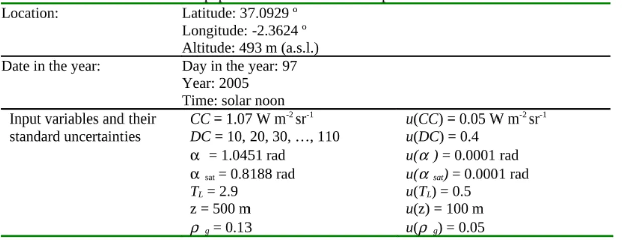
The specific time for the evaluation of CSUs by each variable is solar noon of day 97 in 2005 for which the eccentricity of the Earth’s orbit is the unity. Table 1 shows the satellite variables determined for this time, taken from the web site of EUMETSAT on November 14, 2006. Note that the digital count, DC, is left as a “free” variable. In fact, to find out the influence of each of the variables in KC, its whole linear

range must be covered. This is accomplished by covering DC up to 114. This maximum was selected because a higher DC leads to n greater than 0.8, i.e., outside of the linear range of this study, however, most of the DC is within this range. Though the satellite elevation α sat is fixed for a given pixel, it is

variable for a complete image and its influence should be considered. Even though the maximum difference between two values of TL on consecutive days is less than 0.05, it can vary during the day for a

given site. Its uncertainty has been determined as the estimated difference between the real value deduced from beam irradiance data recorded at the PSA station and the daily TL adopted. Similarly, the uncertainty

in z is due to the differences in terrain elevation within the pixel. The pixel including the position of the PSA is a mixed zone, flat over almost all of the area and steeper on the northern edge. The uncertainty in

z is a representative amount of the change in z over the pixel. TL and z are a particular case, because even if it were possible to determine them exactly for a certain location, they are still variable over the area of the pixel. Then even if both variables are correctly assigned in the algorithm, they can lead to wide uncertainty in the result. The rest of the uncertainties were taken from previous experience in method evaluation (EUMETSAT; ESRA, 2000;Lefèvre et al., 2007).

5. Results and discussion

Accepting the values shown in Table 1 as the starting point, ρ α , n, KC and G are computed, as DC is

varied in the interval indicated. As they do not depend on DC, ρ n and GC remain the same in all cases of

the numerical example, as shown in Table 2. Following the uncertainty study outline in Section 3.1, Figure 3 shows the relative changes induced in KC by the input variables that influence it through ρ α ,

ρ g, ρ n, respectively. Figure 3 exhibits negative values because the signs of the sensitivity coefficients

have been retained for better understanding. It may be observed that the changes induced by every variable through both ρ α and ρ n (Figures 3a and 3c) tend to diminish with rising KC, while the change

induced by ρ g stays almost constant at around 5% throughout the interval (Figure 3b). The most relevant

changes induced in KC by ρ α are due to TL, z and CC, and amount to 29%, 18% and 14%, respectively.

In the worst case, the changes induced by the uncertainty in DC, α and α sat do not exceed 1.5%. The same behavior is observed in changes induced by variables through ρ n, reproducing similar figures. They

are the results of the former general law of error propagation. In the next section, uncertainties –not errors– are calculated as actually defined by ISO 1995.

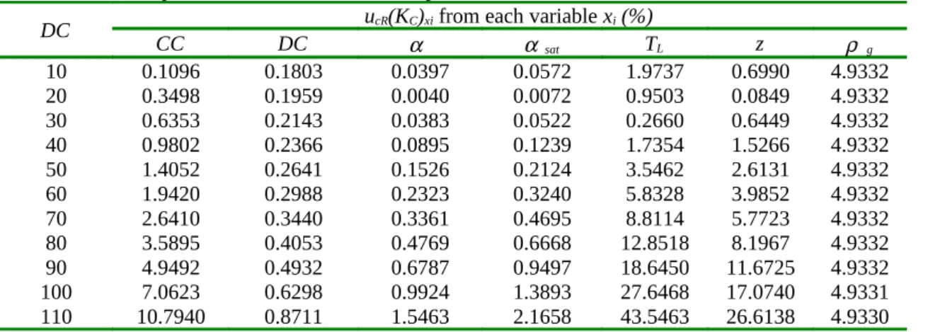
In this section, every partial and total CSU (Equation 7) is computed. The contribution of each individual input variable to partial CSU in KC and G is found by calculating their contributions through ρ α and ρ n.

Note that CC and DC contribute to the CSU through ρ α only. According to Equations (7) and (9), this contribution to CSU by CC, and also DC, is equal to its induced change, except that it is positive. Table 3 and Figure 4a show the relative partial CSU in KC from each input variable, while Table 4 and Figure 4b

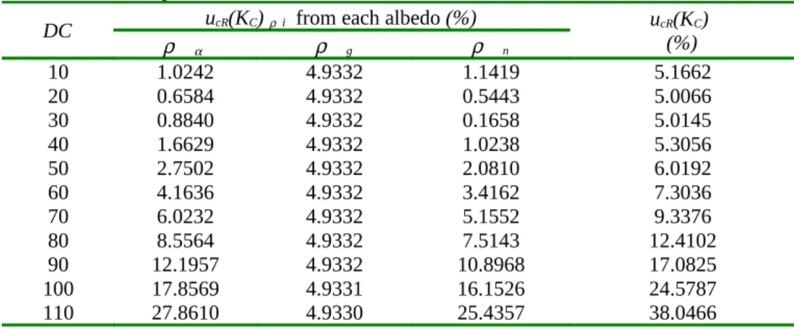
show the corresponding partial CSU of G. Partial CSU due to each albedo, ρ α , ρ g and ρ n, as variables

themselves (ucR(KC) ρi, ρ i = ρ α , ρ g, ρ n ), and the relative total CSU, ucR(KC), are shown in Table 5 and

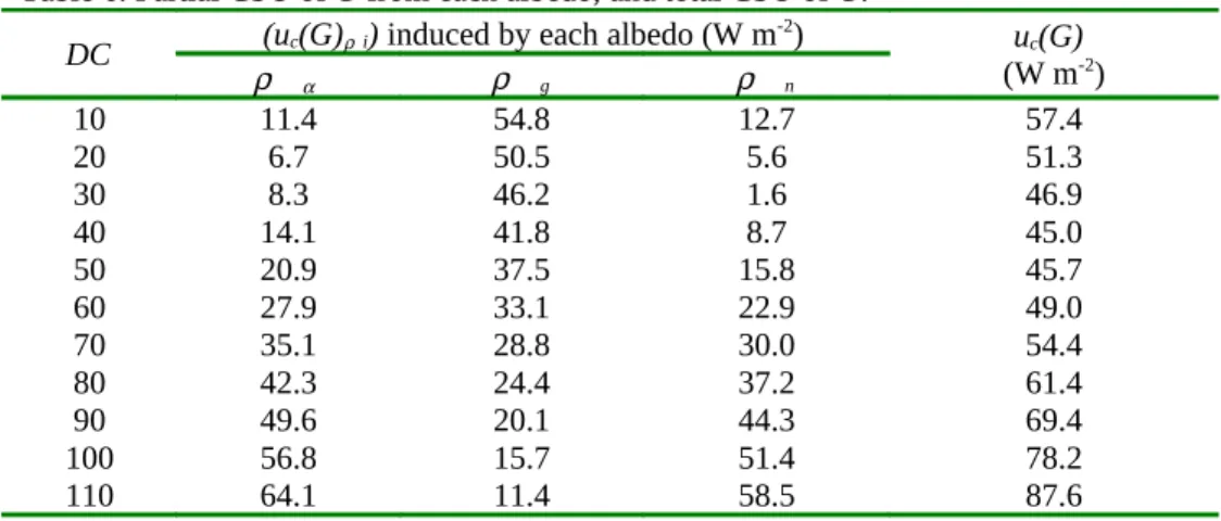
plotted in Figure 5a. The partial CSU of G due to each albedo, uc(G)ρi , and the total CSU of G, uc(G) are

given in Table 6 and plotted in Figure 5b.

Figures 4a and 4b offer similar tendencies. It may be observed that the most important influences occur at low KC, and therefore also low G, that is, under very cloudy skies. Every partial CSU tends to decrease

with rising KC, and so also G, except for ρ g which remains constant throughout the interval for KC

(Figure 4a) and increases linearly with G (Figure 4b). The partial CSU due to DC or α or α sat is less

than 3% (Figure 4a), or 5 W m-2 _{(Figure 4b) in the least favorable case. α and α}

sat are well-known

variables evaluated by many authors (Walraven, 1978; Wilkinson, 1983; Holland and Mayer, 1988; Blanco-Muriel et al., 2001). The models proposed by these authors are very accurate for those angles dealt with by the Heliosat-2 method, i.e., greater than 15º (Rigollier et al., 2004; Lefèvre et al., 2007), and this explains the small partial CSU. More attention should be given to the partial CSU due to CC at low

KC (15% in Figure 4a) and low G (26 W m-2 _{in Figure 4b), or z (35%, 60 W m}-2_{, respectively), or ρ}

g (5%,

10 W m-2 _{respectively) and T}

L (55%, 100 W m-2, respectively), which are high due to the uncertainty

associated with each variable. The uncertainty in z is already 20% of the variable itself (Table 1) and this is reflected in its total influence. The uncertainty in z is particularly easy to reduce with the aid of geographic information systems, which are increasingly accurate and compatible with all information systems. The uncertainty in ρ g comes from the difficulty in assessing it from a time-series of reflectances

for mixed cases of clear and cloudy skies (Cano et al., 1986; Diabaté et al., 1988; Stuhlmann et al. 1990; Perez et al., 2002; Rigollier et al., 2004). In addition, the assessment strategy plays a role in the uncertainty, as discussed by Lefèvre et al. (2007), who select only one ρ g per month, although this can

vary more rapidly (Diabaté et al., 1989a). Making a more dynamic selection of ρ g would reduce its

uncertainty and thereby narrow the uncertainty interval in KC due to this variable. The calibration

coefficient, CC, is very important, as it occurs in all procedures involving measurement. The authors of the Heliosat-2 method and EUMETSAT have given well-deserved attention to this variable (Lefèvre et al., 2000; Govaerts et al., 2001; Grau et al., 2002; Rigollier et al., 2002). Both methods for estimating CC are dynamic and describe its variations in high time resolution, resulting in a CC estimation with an acceptable relative partial CSU (less than 15% of KC). The most significant partial CSU for low KC and

low G is the one due to TL: 55% of KC and 100 W m-2. This factor is in the clear-sky model used and

therefore has a share in calculation of the atmospheric reflectance, terrestrial reference albedo and global irradiance incident on the surface (after calculating KC), through the atmospheric transmittance, for both

the direct and diffuse components. Its many interventions, along with its own uncertainty, make its partial CSU significant. Therefore, it is essential to the Heliosat-2 method that TL be more accurate.

As for the influence of each albedo (Figure 5a), the partial CSU from ρ α is slightly wider than from ρ n

because two more variables, CC and DC, enter in its calculation. The uncertainty of the first is very influential, as already observed. ρ g is included in this figure so its influence on the albedoes above can be

compared. As already seen from the independent input variables, at low KC, relative total CSU is wide,

nearly 50%, while at high KC it drops to around 5%. The close agreement between the relative partial

CSU calculated in this section and the changes induced as shown in the section above may be explained by the mathematical relationship existing between these parameters (see Section 3). The results calculated in this uncertainty study are in agreement with those found by Lefèvre et al. (2007) for ρ g and ρ n. In

absolute terms (Figure 4b), the partial CSU from ρ g behaves differently from the rest of the independent

variables, because, contrary to the others, it continues growing over the entire interval. The total CSU in the estimation of G (Figure 5b) reaches its maximum with low irradiance, i.e., with cloudy skies, mostly because of the contributions of TL, z and CC. Then total CSU decreases with increasing G down to its

minimum, and increases with higher irradiance due to the growing contribution of ρ g as the sky becomes

clearer.

6. Conclusions

This article deals with the uncertainties in the Heliosat-2 method for estimating the SSI. The ISO 1995 standard procedure was used in four steps. Firstly, the changes induced by the input variables, formerly called the general law of error propagation, were calculated by studying each albedo separately. Secondly, the partial CSU from each variable was calculated, combining its effect through any albedo. Thirdly, the partial CSU of KC from each albedo is calculated, and fourthly, the total CSU of KC and G

was calculated. With both the partial and total analysis of CSU from the input variables, it was found that, at low KC, i.e., for cloudy skies, TL, z, CC and ρ g are the most influential agents in the final uncertainty,

while the influence of the other variables, DC, α and α sat, are negligible. The total CSU amounts to

90 W m-2 _{for low K}

C, i.e., 50% of KC. It decreases with growing KC, down to a minimum of 45 W m-2

when skies are clear (KC = 0.88). However, since the contribution of ρ g increases linearly (Figure 5b),

total CSU increases again, reaching a second maximum of 60 W m-2_{, i.e., approximately 5% of K}

C. These

results agree with those found by Lefèvre et al. (2007).

This study shows some areas in which Heliosat-2 could be improved. Among the variables found to be most important, the intrinsic uncertainty of z and ρ g shows some potential for reduction. The database

TerrainBase (1995) used by Rigollier et al. (2004) offers global coverage with a cell size of 5’ of arc angle (approximately 10 km at mid latitude). More accurate terrain elevation models, such as SRTM (Van Zyl, 2001) are now available. Using such advanced models will reduce the intrinsic uncertainty of z at a given site. The strategy for determining ρ g is rather important to the CSU. A better description of its

behavior over time as proposed by Hammer (2000), Perez et al. (2002), Zelenka (2003) should reduce the intrinsic uncertainty of ρ g, thus improving the assessment of KC over the whole range. Uncertainty of TL

affects the CSU more than any other variable, not only because of its own wide uncertainty, but also because it enters in numerous intermediate calculations as well. Therefore, accurate knowledge of TL is

fundamental to decreasing the CSU. It should be kept in mind that the estimated KC found is neither over

nor underestimated in these proportions, which are the intervals of uncertainty in which it is found.

Acknowledgements

The authors sincerely thank the four anonymous reviewers for their comments and suggestions which greatly improve the readability and clarity of this article.

References

Beyer, H.G., Costanzo, C., Heinemann, D., 1996. Modifications of the Heliosat procedure for irradiance estimates from satellite images. Solar Energy 56, 207-212.

Blanco-Muriel, M., Alarcón-Padilla, D.C., López-Moratalla, T., Lara-Coria, M., 2001. Computing the solar vector. Solar Energy 70, 431-441.

Bois, B., Pieri, P., Van Leeuwen, C., Wald, L., Huard, F., Gaudillère, J.P., Saur, D., 2008. Using remotely sensed solar radiation data for reference evapotranspiration estimation at daily time step. Agricultural and Forest Meteorology 148, 619-630.

Cano, D., Monget, J.M., Albuisson, M., Guillard, H., Regas, N., Wald, L., 1986. A method for the determination of the global solar radiation from meteorological satellite data. Solar Energy 37, 31-39. Cros, S., 2004. Création d’une climatologie du rayonnement solaire incident en ondes courtes a l’aide d’images satellitales. PhD Thesis. Ecole des mines de Paris, Paris, France, pp. 44-47, 155 P.

Diabaté L., Michaud-Regas N., Wald L., 1989a. Mapping the ground albedo of Western Africa and its time evolution during 1984 using Meteosat visible data. Remote Sensing of Environment, 27, 3, 211-222. Diabaté L., Moussu G., Wald L., 1989b. Description of an operational tool for determining global solar radiation at ground using geostationary satellite images. Solar Energy, 42, 3, 201-207.

Diabaté, L., Demarcq, H., Michaud-Regas, N., Wald, L., 1988. Estimating incident solar radiation at the surface from images of the Earth transmitted by geostationary satellites: the Heliosat Project. International Journal of Solar Energy 5, 261-278.

ESRA, 2000. The European Solar Radiation Atlas. Vol. 2: Database and exploitation software. Edited by: Scharmer, K., Greif, J. Les Presses de l’Ecole des Mines, Paris, France.

EUMETSAT, http://www.eumetsat.int.

Geiger, M., Diabaté, L., Ménard, L., Wald, L. 2002. A web service for controlling the quality of measurements of global solar irradiation. Solar Energy 73, 6, 475-480.

Govaerts, Y.M., Arriaga, A., Schmetz, J., 2001. Operational vicarious calibration of the MSG/SEVIRI solar channels. Advances in Space Research 28, 21-30.

Grau, J., Torres, R., Massons, J., 2002. Drift in the Meteosat-7 VIS channel calibration. International Journal of Remote Sensing 23, 5277-5282.

Grüter, W., Guillard, H., Möser, W., Monget, J. M., Palz, W., Raschke, E., Reinhardt, R. E., Schwarzmann, P., Wald, L., 1986. Solar radiation data from satellite images. Vol. 4. Serie: Solar energy R&D in the European Community, Series F. Reidel Publishing Company.

Hammer, A., 2000. Amwendungsspezifische Solarstrahlungsinformationen aus Meteosat-Daten. PhD Thesis, Farbereich Physik, Carl von Ossietzky University, Oldenburg, Germany. 107 p.

Holland, P.G., Mayer, I., 1988. On calculating the position of the Sun. International Journal of Ambient Energy 9, 47-52.

ISO, 1993. International vocabulary of basic and general terms in metrology, second edition. International Organization for Standardization, Geneva, Switzerland.

ISO, 1995. Guide to the Expression of Uncertainty in Measurement, International Organization of Standardization, Geneva, Switzerland.

Lefèvre, M., Albuisson, M., Wald, L., 2002. Description of the software Heliosat- II for the conversion of images acquired by Meteosat satellites in the visible band into maps of solar radiation available at ground level. Ecole des Mines de Paris – Armines, France.

Lefèvre, M., Bauer, O., Iehlé, A., Wald, L., 2000. An automatic method for the calibration of time-series of Meteosat images. International Journal of Remote Sensing 21, 1025-1045.

Lefévre, M., Wald, L., Diabaté, L., 2007. Using reduced data sets ISCCP-B2 from the Meteosat satellites to assess surface solar irradiance. Solar Energy, 81, 240-253.

Mahmood, R., Hubbard, K.G., 2005. Assessing bias in evapotranspiration and soil moisture estimates due to the use of modelled solar radiation and dew point temperature data. Agricultural and Forest Meteorology 30, 71-84.

Moussu, G., Diabaté, L., Obrecht, D., Wald, L., 1989. A method for the mapping of the apparent ground brightness using visible images from geostationary satellites. International Journal of Remote Sensing 10, 1207 – 1225.

Noia, M., Ratto, C.F., Festa, R., 1993. Solar irradiance estimation from geostationary satellite data: I. Statistical models. Solar Energy 51, 449-456.

Pastre, C., 1981. Développement d’une méthode de détermination du rayonnement solaire global à partir des données Meteosat. La Météorologie, VIe série N 24, mars.

Perez, R., Ineichen, P., Moore, K., Kmiecik, M., Chain, C., George, R., Vignola, F., 2002. A new operational model for satellite-derived irradiances: description and validation. Solar Energy. 73, 307-317. Perez, R., Seals, R., Zelenka, A., 1997. Comparing satellite remote sensing and ground network measurements for the production of site/time specific irradiance data. Solar Energy 60, 89-96.

Raschke, E., Stuhlmann, R., Palz, W., Steemers, T.C., 1991. Solar radiation atlas of Africa. Edited by: Balkema, A. Rotterdam, The Netherlands, 155 p.

Remund, J., Wald, L., Lefèvre, M., Ranchin, T., Page, J., 2003. Worldwinde Linke turbidity information. In Proceedings of ISES Solar Workld Congress, 16-19 June, Göteborg, Sweden. Available in

Reuter H.I., Kersebaum, K.C., Wendroth, O., 2005. Modelling of solar radiation influenced by topographic shading––evaluation and application for precision farming. Physics and Chemistry of the Earth 30, 143-149.

Rigollier, C., Bauer, O., Wald, L., 2000. On the clear sky model of the 4th _{European Solar Radiation Atlas} with respect to the Heliosat method. Solar Energy, 68, 33-48.

Rigollier, C., Lefèvre, M., Blanc, Ph., Wald, L., 2002. The operational calibration of images taken in the visible channel of the Meteosat-series of satellites. Journal of Atmospheric and Oceanic Technology, 19, 1285-1293.

Rigollier, C., Lefèvre, M., Wald, L., 2001. Heliosat version 2. Integration and exploitation of networked Solar Radiation Databases for environment monitoring (SoDa Project). Contract Number: ST-1999-12245, pp.1-94. Available at www.soda-is.com/doc/heliosat2_d3.pdf.

Rigollier, C., Lefèvre, M., Wald, L., 2004. The method Heliosat-2 for deriving shortwave solar radiation from satellite images. Solar Energy 77, 159-169.

Rigollier, C., Wald, L., 1998. Using Meteosat images to map the solar radiation: improvements of the Heliosat method. In Proceedings of the 9th _{Conference on Satellite Meteorology and Oceanography.} Published by Eumetsat, Darmstadt, Germany, EUM P 22, pp. 432-433.

Şen, Z., 2004. Solar energy in progress and future research trends. Progress in Energy and Combustion Science 30, 367-416.

Speranza, A., van Geel, B., van der Plicht, J., 2003. Evidence for solar forcing of climate change at ca. 850 cal BC from a Czech peat sequence. Global and Planetary Change 35, 51-65.

Stuhlmann, R., Rieland, M., Raschke, E., 1990. An improvement of the IGMK model to derive total and diffuse solar radiation at the surface from satellite data. Journal of Applied Meteorology 29, 596-603. TerrainBase, 1995. Worldwide Digital Terrain Data, Documentation Manual, CD-ROM Release 1.0, April 1995, NOAA, National Geophysical Data Center, Boulder, CO, USA.

Van Zyl, J., 2001. The shuttle Radar Topography Mission (SRTM): a breakthrough in remote sensing of topography. Acta Astronautica 48, 559-565.

Vera, N., 2005. Atlas climático de irradiación solar a partir de imágenes del satélite NOAA. Aplicación a la Península Ibérica. Tesis doctoral. Universidad Politécnica de Cataluña, Spain. 283P.

Walraven, R., 1978. Calculating the position of the sun. Solar Energy 20, 393. Revised by Archer, C.B., 1980. Solar Energy 25, 91.

Wilkinson B.J., 1983, The effect of atmospheric refraction on the solar azimuth. Solar Energy 30, 295. Zarzalejo, L.F., 2006. Irradiancia solar global horaria a partir de imágenes de satélite. Serie: Colección Documentos CIEMAT. Ed. CIEMAT, Madrid, Spain.

Zelenka, A., 2003. Progress in estimating insolation over snow covered mountains with Meteosat VIS-channel: a time series approach. In: Proceedings of the 3rd _{Workshop on Satellites for Solar Energy,} University of Geneva, Switzerland, March 19-21, 2003.

Zelenka, A., Perez, R., Seals, R., Renné, D., 1999. Effective accuracy of satellite-derived hourly irradiances. Theoretical and Applied Climatology 62, 199-207.

Table 1. Conditions used in this paper for the numerical example.

Location: Latitude: 37.0929 º

Longitude: -2.3624 º Altitude: 493 m (a.s.l.) Date in the year: Day in the year: 97

Year: 2005 Time: solar noon Input variables and their

standard uncertainties CC = 1.07 W m-2 _sr-1 DC = 10, 20, 30, …, 110 α = 1.0451 rad α sat = 0.8188 rad TL = 2.9 z = 500 m ρ g = 0.13 u(CC) = 0.05 W m-2 _sr-1 u(DC) = 0.4 u(α ) = 0.0001 rad u(α sat) = 0.0001 rad u(TL) = 0.5 u(z) = 100 m u(ρ g) = 0.05

1

Table 2. ρ α , n, KC and G for the DC tested and fixed ρ n and GC. DC ρ α n KC G (W m-2) 10 -0.0360 -0.1646 1.1646 1112 20 0.0576 -0.0722 1.0722 1024 30 0.1512 0.0201 0.9799 936 40 0.2448 0.1125 0.8875 847 50 0.3384 0.2048 0.7952 759 60 0.4320 0.2972 0.7028 671 70 0.5256 0.3895 0.6105 583 80 0.6192 0.4819 0.5181 495 90 0.7128 0.5742 0.4258 406 100 0.8064 0.6666 0.3334 318 110 0.9000 0.7589 0.2411 230 ρ n = 1.1443 GC = 955 W m-2

1

Table 3. Relative partial CSU of KC from each input variable.

DC _{CC DC} ucR(KC)xi from each variable xi (%)

α α sat TL z ρ g 10 0.1096 0.1803 0.0397 0.0572 1.9737 0.6990 4.9332 20 0.3498 0.1959 0.0040 0.0072 0.9503 0.0849 4.9332 30 0.6353 0.2143 0.0383 0.0522 0.2660 0.6449 4.9332 40 0.9802 0.2366 0.0895 0.1239 1.7354 1.5266 4.9332 50 1.4052 0.2641 0.1526 0.2124 3.5462 2.6131 4.9332 60 1.9420 0.2988 0.2323 0.3240 5.8328 3.9852 4.9332 70 2.6410 0.3440 0.3361 0.4695 8.8114 5.7723 4.9332 80 3.5895 0.4053 0.4769 0.6668 12.8518 8.1967 4.9332 90 4.9492 0.4932 0.6787 0.9497 18.6450 11.6725 4.9332 100 7.0623 0.6298 0.9924 1.3893 27.6468 17.0740 4.9331 110 10.7940 0.8711 1.5463 2.1658 43.5463 26.6138 4.9330

1

Table 4. Partial CSU of G from each input variable.

DC uc(G)xi from each variable xi (W m

-2₎ CC DC α α sat TL z ρ g 10 1.2 2.0 0.4 0.6 21.9 7.8 54.8 20 3.6 2.0 0.0 0.1 9.7 0.9 50.5 30 5.9 2.0 0.4 0.5 2.5 6.0 46.2 40 8.3 2.0 0.8 1.1 14.7 12.9 41.8 50 10.7 2.0 1.2 1.6 26.9 19.8 37.5 60 13.0 2.0 1.6 2.2 39.1 26.7 33.1 70 15.4 2.0 2.0 2.7 51.4 33.6 28.8 80 17.8 2.0 2.4 3.3 63.6 40.5 24.4 90 20.1 2.0 2.8 3.9 75.8 47.4 20.1 100 22.5 2.0 3.2 4.4 88.0 54.3 15.7 110 24.8 2.0 3.6 5.0 100.2 61.3 11.4

1

Table 5. Relative partial CSU of KC from each albedo, and relative total CSU of KC. DC ucR(KC) ρi from each albedo (%) ucR(KC) _(%)

ρ α ρ g ρ n 10 1.0242 4.9332 1.1419 5.1662 20 0.6584 4.9332 0.5443 5.0066 30 0.8840 4.9332 0.1658 5.0145 40 1.6629 4.9332 1.0238 5.3056 50 2.7502 4.9332 2.0810 6.0192 60 4.1636 4.9332 3.4162 7.3036 70 6.0232 4.9332 5.1552 9.3376 80 8.5564 4.9332 7.5143 12.4102 90 12.1957 4.9332 10.8968 17.0825 100 17.8569 4.9331 16.1526 24.5787 110 27.8610 4.9330 25.4357 38.0466

1

Table 6. Partial CSU of G from each albedo, and total CSU of G.

DC _ρ (uc(G)ρi) induced by each albedo (W m-2) _{(W m}uc(G) -2₎

α ρ g ρ n 10 11.4 54.8 12.7 57.4 20 6.7 50.5 5.6 51.3 30 8.3 46.2 1.6 46.9 40 14.1 41.8 8.7 45.0 50 20.9 37.5 15.8 45.7 60 27.9 33.1 22.9 49.0 70 35.1 28.8 30.0 54.4 80 42.3 24.4 37.2 61.4 90 49.6 20.1 44.3 69.4 100 56.8 15.7 51.4 78.2 110 64.1 11.4 58.5 87.6

2

Figure 1. Relationship between the clear-sky index KC and cloud index n (Equation 2).

Figure 2. (a) Values for DC in 2004 and 2005; (b) Relative frequency histogram for DC in the same period. In this numerical example, DC greater than 114 leads to n over 0.8 (cloudy skies), i.e., outside of the range of this study; (c) Periodic annual series for TL; (d) Values for ρ g in 2004 and 2005.

Figure 3. (a) Relative change in KC, by the variables influencing it through ρ α. (b) As a), but for ρ g. (c)

As a), but for variables influencing the relative change in KC through ρ n.

Figure 4. (a) Relative partial CSU of KC and (b) partial CSU of G, from each independent variable.

Figure 5. (a) The relative partial CSU of KC by ρ α , ρ g and ρ n and relative total CSU of KC. (b) The

partial CSU of G due to each albedo, and the total CSU of G.

Figure 1

(a) (b)

(c) (d)

Figure 2.

(a)

(b)

(c) Figure 3.

(a)

(b) Figure 4.

(a) (b) Figure 5.