HAL Id: hal-02943480
https://hal.archives-ouvertes.fr/hal-02943480
Submitted on 23 Sep 2020
HAL is a multi-disciplinary open access
archive for the deposit and dissemination of
sci-entific research documents, whether they are
pub-lished or not. The documents may come from
teaching and research institutions in France or
abroad, or from public or private research centers.
L’archive ouverte pluridisciplinaire HAL, est
destinée au dépôt et à la diffusion de documents
scientifiques de niveau recherche, publiés ou non,
émanant des établissements d’enseignement et de
recherche français ou étrangers, des laboratoires
publics ou privés.
FACTORIZATION FOR ACOUSTIC SCENE
CLASSIFICATION
Victor Bisot, Romain Serizel, Slim Essid, Gael Richard
To cite this version:
Victor Bisot, Romain Serizel, Slim Essid, Gael Richard. SUPERVISED NONNEGATIVE MATRIX
FACTORIZATION FOR ACOUSTIC SCENE CLASSIFICATION. IEEE international evaluation
campaign on detection and classification of acousitc scenes and events (DCASE 2016), Sep 2016,
Budapest, Hungary. �hal-02943480�
SUPERVISED NONNEGATIVE MATRIX FACTORIZATION FOR ACOUSTIC SCENE
CLASSIFICATION
Victor Bisot, Romain Serizel, Slim Essid and Gael Richard
LTCI, CNRS, T´el´ecom ParisTech, Universit´e Paris-Saclay, 75013, Paris, France
ABSTRACT
This report describes our contribution to the 2016 IEEE AASP DCASE challenge for the acoustic scene classification task. We pro-pose a feature learning approach following the idea of decomposing time-frequency representations with nonnegative matrix factoriza-tion. We aim at learning a common dictionary representing the data and use projections on this dictionary as features for classification. Our system is based on a novel supervised extension of nonnegative matrix factorization. In the approach we propose, the dictionary and the classifier are optimized jointly in order to find a suited represen-tation to minimize the classification cost. The proposed method sig-nificantly outperforms the baseline and provides improved results compared to unsupervised nonnegative matrix factorization.
Index Terms— Acoustic Scene Classification, Feature learn-ing, Matrix Factorization
1. INTRODUCTION
The Acoustic Scene Classification problem (ASC) has mainly been addressed by finding the features that can best represent the scenes. Many works, including some submissions to the last edition of the challenge, considered the use of speech inspired features such as Mel Frequency Cepstral Coefficients combined with other low level features (zero-crossing rate, spectral centroid,...) [1]. Another no-table trend has been to extract image processing features from time-frequency images such as histograms of oriented gradients [2, 3]. The main drawback of such hand crafted features is their lack of flexibility as, by definition, they focus on describing a specific as-pect of the signal. Instead, many other sound classification tasks benefited from the success of feature learning techniques in order to learn adapted representations of the data. For example, in ASC, some works successfully proposed the use of unsupervised feature learning techniques such as nonnegative matrix factorization (NMF) [4, 5].
Our system further exploits the advantages of NMF for feature learning when compared to conventional hand crafted features. Af-ter building a time-frequency representation of the data, NMF is applied to jointly learn a dictionary and an activation matrix. The activation matrix contains the projection of the data on the learned dictionary and will be used as the learned features as detailed in [5]. In ASC, NMF is usually applied in an unsupervised setting, meaning the labels are not used during the decomposition step. The method we propose corresponds to a supervised extension of the NMF model which takes advantage of the scene labels to get a de-composition that will help discriminating the scenes. It mainly ex-tends the Task-driven dictionary learning (TDL) model proposed
This work was partly funded by the European Union under the FP7-LASIE project (grant 607480)
in [6]. The TDL model aims at learning a representation which will minimize the classification cost by jointly optimizing the dic-tionary and a binary classifier in a common problem. We propose a novel extension of the general TDL model which links the NMF de-composition to a multinomial logistic regression classifier. We also present our modification of the TDL algorithm used to generate the predictions for our submission to the challenge.
2. DATA MATRIX CONSTRUCTION
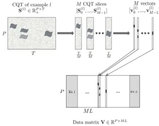
In this section, we describe the construction of the data matrix used as the input representation of the supervised feature learning step. It is identical to the one we presented in [5]. The different data matrix construction steps are illustrated in Figure 1.
2.1. Time-frequency representation
The time-frequency representations of the scene recordings are ex-tracted from the signals using a Constant Q-transform (CQT). We denote S ∈ RP ×T+ as the CQT transform of a given recording,
where T is the number of time frames and P is the number of fre-quency bands. Without loss of generality, the recordings are as-sumed to have equal length, which is the case for the challenge dataset.
2.2. Spectrogram pooling
In order to construct the data matrix from the time frequency im-ages, we apply two simple slicing and pooling steps. They aim at reducing the dimensionality of the data while providing a suited representation to the feature learning step. To do so, we start by dividing each time frequency image into M non-overlapping slices of length Q = T /M . We use Sm to denote the Q-frames long
spectrogram slice starting Q × m frames after the beginning of the recording. The CQT image S is now considered as a set of con-secutive shorter spectrograms S = [S0, ..., SM −1]. Each of the M
spectrogram slices are then averaged over time resulting in M vec-tors. Assuming we have L training examples, every recording is now represented by a set of vectors V(l) = [v(l)0 , ..., v
(l)
M −1] where
v(l)m is a vector of size P obtained by averaging the slice S (l) m over
time. We extract the L sets of vectors V(l)in the training set and stack them column-wise to build the data matrix V ∈ RP ×N+ , where
V = [V(1), ..., V(L)] and N = M L.
3. SUPERVISED NONNEGATIVE MATRIX FACTORIZATION
In this section, we first briefly present the unsupervised NMF and Sparse NMF problems. Then, we present the supervised dictionary
… …
Figure 1: Building steps of the data matrix V, input representation for the matrix factorizations
model (TDL) in its original formulation. Finally, we propose some modifications to the model and the algorithm.
3.1. Nonnegative matrix factorization for unsupervised learn-ing
3.1.1. Original formulation
Nonnegative matrix factorization is a well known technique [7] to decompose nonnegative data into nonnegative dictionary elements. Many problems benefit from the nonnegative aspect of the decom-position to learn better representations of the data, especially in the audio processing field. In NMF, the goal is to find a decomposition that approximates a data matrix V ∈ RP ×N+ such as V ≈ WH with
W ∈ RP ×K+ and H ∈ R K×N
+ . The matrix W corresponds to the
dictionary of basis vectors and the matrix H is the activation matrix containing the projections of V on the dictionary. NMF is obtained solving the following optimization problem:
min
W,HDβ(V|WH) s.t. W, H ≥ 0, (1)
where Dβis a separable divergence which is commonly chosen to
be the β-divergence [8].
3.1.2. Sparse NMF
Sparsity is often desired in matrix factorization in order to provide a more robust and interpretable decomposition. We present the sparse NMF formulation as proposed in [9] but there are many other ways of enforcing sparsity in NMF. Here, a l1-norm penalty term on the
activation matrix H is added to the problem while a unit l2-norm
constraint is applied on the dictionary elements. The matrices W and H are the solution of the following problem:
min W,H≥0 X i Dβ(vi, X k hki wk kwkk2 ) + λ1 X i,k hik, (2)
where wkis the dictionary column indexed by k, 1 ≤ k ≤ K.
3.2. Supervised learning with nonnegative matrix factorization 3.2.1. Task-driven dictionary learning model
The general idea of TDL is to group the dictionary learning and the training of the classifier in a joint optimization problem. Influenced by the classifier, the basis vectors are encouraged to explain the dis-criminative information in the data while keeping a low reconstruc-tion cost. The TDL model first considers the optimal projecreconstruc-tions h?(v, W) of the data point v on the dictionary W. The projections are defined as solutions of the elastic-net problem [10] expressed as: h?(v, W) = min h∈RK 1 2kv − Whk 2 2+ λ1khk1+ λ2 2 khk 2 2. (3)
Given each data point v is associated with a label y in a fixed set of labels Y, a classification loss ls(y, A, h?(v, W)) is defined, where
A are the parameters of the classifier. The TDL problem is now expressed a joint minimization in W and A of the expected classifi-cation cost: min W∈W,Af (W, A) + ν 2kAk 2 2, (4) with f (W, A) = Ey,v[ls(y, A, h?(v, W)]. (5)
Here, W is defined as the set of dictionaries containing unit l2norm
basis vectors and ν is a regularization parameter on the classifier’s parameters to prevent over fitting. The problem in equation (5) is optimized with stochastic gradient descent. After randomly draw-ing a data point v, the optimal projection h?(v, W) is first com-puted. Then, the dictionary W and the classifier parameters A are updated by projected gradient. We refer the interested reader to [6] for a more complete description of the model.
3.2.2. Adapting to the task
The original formulation supposes each projection h?(v, W) is classified individually. Instead, we want to classify the mean of the projections of the data points v(l)belonging to the sound example
l ∈ [[1, L]] with V(l) = [v(l) 0 , ..., v
(l)
M −1] (see section 2.2). We
de-fine h(l)as the averaged projection of V(l)on the dictionary, where
h(l) = 1 M
PM m=1h
?(v(l)
m, W). Thus, the classification expected
cost is now expressed as:
f (W, A) = Ey,V[ls(y, A, h(l))]. (6)
This alternate formulation only slightly modifies the gradients of f (W, A) with respect to W and A. The other changes include:
• The application of the model for the multinomial logistic re-gression classification case. Compared to the two class formu-lation chosen in [6], it has the advantage of learning a common dictionary for all the labels instead of relying on a one-versus-all strategy. Expressing the gradients of f with respect to W for the multi-logit cost is rather straightforward.
• A nonnegative version of the problem. Although it was men-tioned as possible by the authors in [6], it has not been applied and leads to improved results in our case.
3.2.3. Modified algorithm
We also propose a slight change in the algorithm proposed in [6] which we found easier to tune and provided better results for our
problem. The changed algorithm is presented in Algorithm 1. It alternates between an update of the classifier using the full set of projections and an update of the dictionary by stochastic projected gradient on a full epoch. An epoch is defined as a full pass through a random permutation of the training set resulting in the number of iterations I being the number of passes through the data. The multinomial logistic regression parameters A are no longer updated with stochastic gradient descent but with one iteration of the L-BFGS algorithm [11] using the full set of averaged projections in H?(V, W) = [h(1), ..., h(L)]. Here, ∇Wls(y, A, h?) is the
gradi-ent of the classification cost with respect to the dictionary W and ρ is the projected gradient step. The operation ΠWis the projection
on W, the set of nonnegative dictionaries with unit `2norm basis
vectors.
Algorithm 1 Modified algorithm for the nonnegative TDL model Require: V, W ∈ W, A, λ1, λ2, ν, I, ρ for i = 1 to I do ∀l ∈ [[1, L]] compute h(l) = M1 PM m=1h ? (v(l)m, W) Set H?(V, W) = [h(1), ..., h(L)]
Update A with one iteration of L-BFGS for n = 1 to N do
Draw a random data point v and its label y Compute h?= h?(v, W) Compute ∇Wls(y, A, h?) as in [6] W ← ΠW[W − ρ∇Wls(y, A, h?)] end for end for return W, A
4. EVALUATION ON THE DEVELOPMENT SET
In this section, we evaluate the proposed system on the challenge development set. The results are given in average classification ac-curacy over the same 4 train-test folds provided by the organizers.
4.1. Time-frequency representation extraction
The CQT were extracted with the YAAFE toolbox [12] after normal-izing the signals. The CQT is computed using 24 frequency bands per octave from 5 to 22050 Hz resulting in P = 291 frequency bands. The recordings are 30 seconds long, the CQT are extracted using 30 ms windows without overlap resulting in T = 1000 time frames. In order to build the data matrix (see Section 2.2), we use 1-s long slices leading to M = 30 slices per example. A square root compression is applied to the data matrix followed by a scaling to unit variance.
4.2. Results with the nonnegative TDL
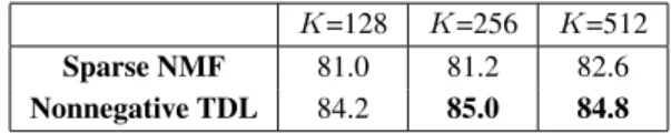
The results obtained when applying the nonnegative TDL to per-form supervised matrix factorization are presented in Table 1. We also include the results obtained with the sparse NMF formulation given in equation (2), which can be seen as the nonnegative TDL’s unsupervised counterpart. Here, Dβis the Euclidean distance
cor-responding to β = 2. We also use Sparse NMF to initialize the dictionaries for the TDL model. The weights of the classifier are initialized by applying the multinomial logistic regression to the projections on the initialized dictionary. In the proposed algorithm,
K=128 K=256 K=512 Sparse NMF 81.0 81.2 82.6 Nonnegative TDL 84.2 85.0 84.8
Table 1: Accuracy scores for the nonnegative TDL model compared to the Sparse NMF results on different dictionary sizes K
the projections on the dictionary (corresponding to equation (3)) are computed using the lasso function from the spams toolbox [13], which also supports nonnegative projections. Then, the classifier (a logistic regression) is updated using one iteration of the scikit-learn [14] implementation of the logistic regression updated with the L-BFGS algorithm. The model is trained on I = 10 iterations with a ρ = 0.001 initial gradient step for the dictionary update. We apply the same heuristic for the decaying over iterations of the gradient step as suggested in [6]. For the different regularization parameters, λ1= 0.2, λ2= 0 and ν = 10 were found to be good values on the
development set.
The results in Table 1 show that the proposed supervised NMF performs better than the Sparse NMF for all dictionary sizes. It also has the advantage of learning good representations for lower dictionary sizes, reaching a 84.2% accuracy for K = 128.
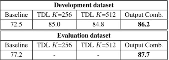
4.3. Final system: combining the outputs
In this section we present the final system used to predict the output labels submitted to the challenge. Most NMF variants are known to be sensitive to initialization, its also the case for the nonnegative TDL model. Therefore, in order to improve the robustness of our system, we propose to combine the outputs of several occurrences of the algorithm. To do so, we apply the nonnegative TDL model to learn a set of 4 different dictionaries W = [W1...W4]. We then
apply the following steps:
• Learn W1and W2on two different initializations for K = 256
and W3and W4on two different initializations for K = 512
• Compute the optimal projections on each dictionary
• Fit a multinomial logistic regression to each of the projection matrices.
• Average the log-probabilities outputs of each classifier • For each test data point: predict the final label by choosing the
one with the highest average log-probability
The final results obtained by combining the outputs are pre-sented in Table 2. The proposed combination slightly improves the performance when compared to individual occurrences of the model on the development dataset. It allows us to take advantage of the slight randomness of the model by providing more robust results. The proposed system also significantly improves the baseline re-sults by reaching a 86.2% accuracy on the development dataset and a 87.7% accuracy on the evaluation dataset. The confusion matrix for the output combination on the development dataset is presented in Table 3. We can see that most confusions are between classes with similar backgrounds or containing many acoustic events of the same nature. For example, our system confuses Residential Area with Park as well as Home with Office. The rest of the classes are classified rather easily.
Bus Bea. C\R Car CC FP GS Home Lib. MS Off. Park RA Tra. Tram Beach 67 0 0 0 0 0 0 0 0 0 0 2 3 0 0 Bus 0 77 1 1 0 0 0 1 0 0 0 0 0 5 0 Caf´e \Restaurant 0 0 60 0 2 0 4 0 0 0 0 0 0 2 0 Car 2 0 0 76 0 0 0 0 0 0 0 0 0 2 5 City center 0 0 1 0 68 1 0 0 0 0 0 7 3 0 0 Forest path 0 0 1 0 0 74 0 0 0 0 0 0 4 0 0 Grocery store 0 0 6 0 0 0 68 0 3 0 0 0 0 0 0 Home 1 0 7 0 0 0 1 74 2 1 9 2 0 1 0 Library 0 0 0 0 0 0 0 2 69 0 0 0 1 2 0 Metro station 0 0 0 0 1 0 5 0 0 77 0 0 0 0 1 Office 0 0 0 0 0 0 0 1 0 0 69 0 0 0 0 Park 0 0 0 0 1 0 0 0 2 0 0 47 18 0 1 Residential Area 7 0 2 0 6 3 0 0 0 0 0 18 49 0 0 Train 0 0 0 0 0 0 0 0 2 0 0 2 0 64 1 Tram 1 1 0 1 0 0 0 0 0 0 0 0 0 2 70
Table 3: Confusion matrix obtained with the output combination system on the development set by reaching a 86.2% accuracy. The rows correspond the true labels and the columns to the predicted labels.
Development dataset
Baseline TDL K=256 TDL K=512 Output Comb. 72.5 85.0 84.8 86.2
Evaluation dataset
Baseline TDL K=256 TDL K=512 Output Comb.
77.2 - - 87.7
Table 2: Accuracy scores obtained by combining the outputs of different occurrences of nonnegative TDL compared to the base-line and the individual nonnegative TDL on two different dictionary sizes.
5. CONCLUSION
We presented the system submitted to the 2016 IEEE AASP DCASE challenge on acoustic scene classification. We proposed a feature learning model based on a supervised extension of nonneg-ative matrix factorization. The resulting supervised model showed improved performance on the development set compared to its un-supervised counterpart. For the final submission, we also combined the outputs of different occurrences of the model in order to learn a more robust representation. The combination of 4 different realiza-tions of the nonnegative TDL model reaches a 86.2% accuracy on the development set.
6. REFERENCES
[1] J. T. Geiger, B. Schuller, and G. Rigoll, “Large-scale audio feature extraction and svm for acoustic scene classification,” in Proc. Workshop on Applications of Signal Processing to Audio and Acoustics, 2013.
[2] A. Rakotomamonjy and G. Gasso, “Histogram of gradients of time-frequency representations for audio scene classifica-tion,” IEEE/ACM Transactions on Audio, Speech and Lan-guage Processing, vol. 23, no. 1, pp. 142–153, 2015. [3] V. Bisot, S. Essid, and G. Richard, “Hog and subband power
distribution image features for acoustic scene classification,” in Proc. European Signal Processing Conference, 2015. [4] E. Benetos, M. Lagrange, and S. Dixon, “Characterisation of
acoustic scenes using a temporally constrained shift-invariant model,” in Proc. Digital Audio Effects, 2012.
[5] V. Bisot, R. Serizel, S. Essid, and G. Richard, “Acoustic scene classification with matrix factorization for unsupervised fea-ture learning,” in Proc. IEEE International Conference on Acoustics, Speech and Signal Processing, 2016.
[6] J. Mairal, F. Bach, and J. Ponce, “Task-driven dictionary learning,” IEEE Transactions on Pattern Analysis and Ma-chine Intelligence, vol. 34, no. 4, pp. 791–804, 2012. [7] D. D. Lee and H. S. Seung, “Learning the parts of objects by
non-negative matrix factorization,” Nature, vol. 401, no. 6755, pp. 788–791, 1999.
[8] C. F´evotte and J. Idier, “Algorithms for nonnegative matrix factorization with the β-divergence,” Neural Computation, vol. 23, no. 9, pp. 2421–2456, 2011.
[9] J. Eggert and E. K¨orner, “Sparse coding and nmf,” in Proc. IEEE International Joint Conference on Neural Networks, vol. 4, 2004, pp. 2529–2533.
[10] H. Zou and T. Hastie, “Regularization and variable selection via the elastic net,” Journal of the Royal Statistical Society: Series B (Statistical Methodology), vol. 67, no. 2, pp. 301– 320, 2005.
[11] D. C. Liu and J. Nocedal, “On the limited memory bfgs method for large scale optimization,” Mathematical program-ming, vol. 45, no. 1-3, pp. 503–528, 1989.
[12] B. Mathieu, S. Essid, T. Fillon, J. Prado, and G. Richard, “Yaafe, an easy to use and efficient audio feature extraction software.” in Proc. International Society for Music Informa-tion Retrieval, 2010, pp. 441–446.
[13] J. Mairal, F. Bach, J. Ponce, and G. Sapiro, “Online learning for matrix factorization and sparse coding,” The Journal of Machine Learning Research, vol. 11, pp. 19–60, 2010. [14] F. Pedregosa, G. Varoquaux, A. Gramfort, V. Michel,
B. Thirion, O. Grisel, M. Blondel, P. Prettenhofer, R. Weiss, V. Dubourg, et al., “Scikit-learn: Machine learning in python,” The Journal of Machine Learning Research, vol. 12, pp. 2825–2830, 2011.