TH `
ESE
TH `
ESE
En vue de l’obtention du
DOCTORAT DE L’UNIVERSIT´
E DE
TOULOUSE
D´elivr´e par : l’Universit´e Toulouse 3 Paul Sabatier (UT3 Paul Sabatier)
Pr´esent´ee et soutenue le 14 Novembre 2014 par :
Fabien Carminati
´
Etude de la variabilit´
e de la vapeur d’eau dans la haute
troposph`
ere-basse stratosph`
ere tropicale et du monoxyde
de carbone troposph´
erique `
a partir d’observations spatiales.
JURY
Jean-Luc ATTI ´E Professeur d’Universit´e Pr´esident du Jury
Michelle SANTEE Directrice de Recherche Rapporteur
Peter HAYNES Professeur d’Universit´e Rapporteur
Philippe RICAUD Directeur de Recherche Directeur de Th`ese
Juying WARNER Charg´ee de recherche Directeur de Th`ese
J.-P. POMMEREAU Directeur de Recherche Examinateur
Emmanuel RIVI `ERE Maˆıtre de Conf´erences Examinateur
´
Ecole doctorale et sp´ecialit´e :
SDU2E : Oc´ean, Atmosph`ere et Surfaces Continentales
Unit´e de Recherche :
CNRM GAME M´et´eo-France CNRS UMR3589
Directeur(s) de Th`ese :
Abstract
The Tropical Tropopause Layer (TTL) is a key region of the atmosphere where abundance of water vapor (H2O) can impact the stratospheric entry and affects the
surface energy balance as well as the stratospheric ozone chemistry. In this thesis, I address the important question of the impact of deep convection on the H2O
variability in the TTL. The implication of the daytime and nighttime difference of the Microwave Limb Sounder (MLS) H2O, cloud Ice Water Content (IWC), and
temperature measurements is investigated from 2005 to 2012 in the tropics and over restricted areas of north and south tropical South America, Africa, maritime continent, and western Pacific. This approach emphasizes the different convec-tive characteristics over land compared to ocean, northern tropics compared to southern tropics, and winter compared to summer. Unlike in oceanic areas, the continental convection is shown to drive the H2O diurnal variability in the TTL
where the sublimation of ice crystals injected by overshoots has a moistening effect up to 80 hPa during the most convective period, and with a greater efficiency in the southern tropics. As part of the TRO-pico project which aims to monitor H2O
in the TTL and Lower Stratosphere (LS), I also emphasize the results obtained for the southern Brazilian region of Bauru.
Like water vapor, carbon monoxide (CO) is also a widely used tracer of convec-tion. Released from incomplete combustion of anthropogenic and natural sources, CO can be detected up to the LS, although its short lifetime prevents a homoge-neous global mixing. In this thesis, and in collaboration with the University of Maryland, I analyzed more than 10 years of CO emission in both hemispheres, over land and ocean, derived from the Atmospheric InfraRed Sounder (AIRS) measure-ments. The high correlation r (r > 0.8) found when compared to emission inven-tory databases demonstrates the viability of the method. Finally, I also outline and validate two new CO products, namely, the sixth version of AIRS CO oper-ational product, and a data fusion combining AIRS and Tropospheric Emission Spectrometer (TES) observations in the troposphere, and AIRS and MLS obser-vations in the Upper Troposphere-Lower Stratosphere (UTLS), providing valuable information for air quality, UTLS dynamics and transport studies.
R´
esum´
e
La haute troposph`ere-basse stratosph`ere tropicale (TTL1) est une r´egion cl´e de l’atmosph`ere o`u l’abondance de vapeur d’eau (H2O) influe sur la quantit´e d’eau
atteignant la stratosph`ere. Les r´epercussions sont de l’ordre radiatif puisque la vapeur d’eau stratosph´erique participe `a l’´equilibre ´energ´etique `a la surface de la Terre, et chimique ´etant donn´e sa propension `a d´egrader l’ozone. Cette th`ese pose donc la question fondamentale du rˆole de la convection profonde sur la variabilit´e de H2O dans la TTL. Pour y r´epondre, les observations de H2O, nuage de glace et
temp´erature produites par l’instrument spatial Microwave Limb Sounder (MLS), `a bord de la plateforme Aura, ont ´et´e analys´ees entre 2005 et 2012 dans les tropiques ainsi que pour des r´egions plus restreintes des tropiques Nord et Sud de l’Am´erique du Sud, l’Afrique, le continent maritime et le Pacifique de l’Ouest. Une approche consistant `a analyser la diff´erence entre les mesures diurnes et nocturnes a permis de mettre en ´evidence les effets de la convection continentale compar´ee `a celle oc´eanique, ainsi que l’influence de l’h´emisph`ere et de la saison. Les r´esultats d´emontrent que la convection continentale est en grande partie `a l’origine de la variabilit´e de H2O dans la TTL grˆace `a l’injection de cristaux de glace qui, suite `a
leur sublimation, hydrate cette r´egion de l’atmosph`ere. Ce ph´enom`ene est observ´e en moyenne jusqu’`a 80 hPa au plus fort de la saison convective et de mani`ere plus marqu´ee dans l’h´emisph`ere Sud. Dans le cadre de TRO-pico, un projet visant `a ´etudier H2O dans la TTL et basse stratosph`ere, une ´etude similaire mais focalis´ee
sur le Sud du Br´esil est aussi pr´esent´ee.
Au mˆeme titre que la vapeur d’eau, le monoxyde de carbone (CO) est aussi couramment utilis´e comme marqueur de convection. Produit par des r´eactions de combustion incompl`etes, aussi bien d’origines naturelles qu’anthropiques, le CO peut ˆetre d´etect´e jusque dans la basse stratosph`ere. Cependant, en raison de sa courte dur´ee de vie, ce gaz n’est pas homog`enement m´elang´e dans l’atmosph`ere. Pour cette th`ese, et en collaboration avec l’universit´e du Maryland, plus de 10 ans d’´emissions de CO obtenues `a partir des observations spatiales de l’Atmospheric InfraRed Sounder (AIRS), `a bord de la plateforme Aqua, ont ´et´e analys´ees en diff´erentiant continents et oc´eans dans chaque h´emisph`ere. La forte corr´elation r
(r > 0.8) obtenue avec les bases de donn´ees d’´emission de CO (GFED et MACCity) a permis de d´emontrer la viabilit´e de la m´ethode. Finalement, deux nouveaux jeux de donn´ees de CO sont pr´esent´es et valid´es, i.e. la fusion de donn´ees combinant les observations de AIRS `a celles du Tropospheric Emission Spectrometer (TES) dans la basse et moyenne troposph`ere et `a celles de MLS dans la haute troposph`ere et au-del`a, ainsi que la sixi`eme et nouvelle version des inversions de AIRS. La forte valeur ajout´ee de ces produits pour les ´etudes li´ees `a la qualit´e de l’air, mais aussi `a la dynamique et au transport dans la haute troposph`ere-basse stratosph`ere est d´emontr´ee dans cette th`ese.
Acknowledgement
To Philippe Ricaud, who not only advised this PhD, but also gave me the oppor-tunity to work in the field of atmospheric science. I learned a lot from him and we shared many good moments in France, Italy, Brazil, and New Zealand.
To Juying Warner, who also advised this PhD and received me in her home labo-ratory as a team member. She did everything to facilitate my integration at the University of Maryland as well as our life in USA.
To Emmanuel Riviere, Jean-Pierre Pommereau, and the TRO-pico team members, who encouraged and counselled my research. They also taught me how small bal-loons are operated during the field campaign in Bauru.
To Michelle Santee and Peter Haynes, for the time that they dedicated to the review of this PhD.
To my beloved parents, sister, and family, who unconditionally supported me all these years.
To my sweet wife, for all her love and support throughout our journeys between France and USA.
Contents
Introduction 13
1 Fundamentals in atmospheric physics and chemistry 21
1.1 Structure of the atmosphere . . . 21
1.2 Atmospheric circulation . . . 23
1.3 Moisture in the atmosphere . . . 26
1.3.1 Saturation and phase changes . . . 27
1.3.2 Tropospheric water vapor . . . 29
1.3.3 Stratospheric water vapor . . . 29
1.4 Carbon in the atmosphere . . . 30
1.4.1 Atmospheric carbon monoxide . . . 31
1.4.2 Impact of CO on climate . . . 34
2 Water vapor monitoring in the tropical tropopause layer from space-borne observations 35 2.1 General introduction . . . 35
2.2 Article 1 - Impact of tropical land convection on the water vapour budget in the tropical tropopause layer . . . 36
2.2.1 Introduction . . . 37
2.2.2 Diurnal water vapour, cloud ice-water content, and temper-ature variability . . . 40
2.2.3 Water vapour seasonal variations over land areas . . . 47
2.2.4 Discussion . . . 51
2.2.5 Conclusions . . . 60
2.3 Summary and perspectives . . . 61
3 The TRO-pico project: a case study at local scale in Southern Brazil 63 3.1 Presentation of TRO-pico . . . 64
3.1.1 Overview . . . 64
3.1.3 Campaigns . . . 67
3.2 Difference between tropical and sub-tropical convective characteris-tics in South America and implications for TRO-pico . . . 68
3.2.1 Southern Brazil, a region of strong convection . . . 68
3.2.2 Climatological background of the Bauru region . . . 72
3.3 In situ measurements preliminary analysis . . . 78
3.3.1 H2O vertical profiles from the Bauru campaigns . . . 78
3.3.2 H2O diurnal cycle in Bauru . . . 80
3.4 Concluding remarks and perspectives . . . 82
4 Analysis of the CO variability in the free troposphere using the Atmospheric InfraRed Sounder AIRS 85 4.1 General introduction . . . 85
4.2 Article 2 - Tropospheric carbon monoxide variability from AIRS under clear and cloudy conditions . . . 87
4.2.1 Introduction . . . 87
4.2.2 Identifying AIRS clear-sky coverage . . . 89
4.2.3 AIRS CO variability for clear sky and cloud-cleared scenes . 92 4.2.4 Distinguishing CO recent emissions from the background us-ing AIRS clear-sky measurements . . . 96
4.2.5 Summary . . . 103
4.3 A method applicable to other instruments: Example of the Infrared Atmospheric Sounding Interferometer IASI . . . 104
4.4 Conclusions and perspectives. . . 108
5 Improving the satellite sensitivity and coverage for CO product 111 5.1 Motivations . . . 111
5.2 Instruments and datasets . . . 113
5.3 Methodology . . . 113
5.3.1 Basic concepts of data assimilation . . . 113
5.3.2 Assimilation applied to AIRS and TES/MLS . . . 115
5.4 Results . . . 116
5.4.1 The AIRS-TES combination in the troposphere . . . 116
5.4.2 The AIRS-MLS combination in the UTLS . . . 119
5.5 Case Study: convective lofting of CO . . . 123
5.6 Conclusions and perspectives. . . 127
6 A first validation of AIRS CO operational product version 6 129 6.1 Overview of the updates in the version 6 of the AIRS retrieval . . . 130
6.1.1 General updates. . . 130
6.2 Impact of the version 6 on the CO product . . . 132
6.2.1 AIRS team estimations . . . 132
6.2.2 CO seasonal and spatial variability . . . 133
6.2.3 Trends and temporal variability . . . 136
6.3 Validation against in situ measurements . . . 138
6.3.1 Airborne campaigns in the Pacific . . . 138
6.3.2 Airborne campaigns in North America . . . 140
6.4 Conclusions and perspectives. . . 147
Conclusions and Perspectives 149
List of Acronyms 159
Appendix A 163
Appendix B 169
Introduction
Without atmosphere, the Earth would be a very hostile place for life. Not even mentioning the oxygen vital for most life-forms, the atmosphere acts as a radia-tion shield stopping most of the harmful solar ultra violet radiaradia-tion. In addiradia-tion, although accounting for less than 1 %, the greenhouse gases that enter in its com-position keep the surface temperature above freezing. Among these gases, one is of particular interest as it is at the heart of most atmospheric processes, having repercussions on a wide variety of fields from the bio-chemistry to the weather and climate (Delmas et al., 2005). This is the water vapor (H2O).
The spectroscopic properties of the water molecule make the water vapor the largest infrared absorber in the atmosphere and consequently the most efficient greenhouse gas. Even so, H2O is not considered as a forcing in the context of
climate change because, unlike long-lived species such as carbon dioxide (CO2),
methane (CH4), and nitrous oxide (N2O), whose concentrations increase with
an-thropogenic emissions, for a given tropospheric temperature the amount of at-mospheric H2O is globally constant. However, the rise of temperature inevitably
leads to a rise of the atmospheric moisture, which can thus absorb more thermal infrared emissions and consequently amplifies the warming by feedback effect.
Although uncertainties exist, modern theories and models have been shown to simulate tropospheric moisture variability, transport, and climate feedback. Re-cent progress has been thoroughly reviewed by Sherwood et al. (2010). In contrast, the contribution of the mechanisms driving the stratospheric water vapor variabil-ity and distribution is still debated and poorly represented in global models. Jiang et al. (2012) identified the upper tropospheric-lower stratospheric (UTLS) H2O
as the constituent with the largest errors and inter-model spread in climate model simulations. This is alarming since the water vapor entering the stratosphere through tropical tropopause layer2 (TTL) is, with the CH
4 oxidation, the major
source of stratospheric H2O and its feedback significantly impacts the climate as it
affects the surface energy budget and stratospheric ozone (O3) chemistry (Solomon
et al., 2010; Dessler et al., 2013). In fact, numerous studies reported an increasing trend of the stratospheric H2O during the 1980s and 1990s (before, too few
servations are available) at a rate of 0.6 % per year (Rosenlof et al., 2001; Scherer et al., 2008; Hurst et al., 2011), followed by a decade without significant trend. This variability is punctuated by sudden drops, like in 1991 (although not well documented), 2000, and more recently, 2011 (Randel et al., 2004; Fueglistaler et al., 2012; Urban et al., 2014). Yet, neither the variability of the tropopause tem-perature (controlling how much the air is dehydrated when it passes through this layer) nor that of the stratospheric CH4 can fully explain the H2O trends or drops.
This further underlines the need to better understand the mechanisms governing the TTL where most of the troposphere-to-stratosphere transport takes place. In 2009, Fueglistaler et al. published a comprehensive overview of the radiative, dy-namical, and chemical processes driving the variability of the TTL structure and constituents, but not without pointing out that some processes, like the deep over-shooting convection, and their impacts on the TTL remain poorly understood. Since then, studies demonstrated the impact of continental overshooting convec-tion on the temperature in the TTL and lower stratosphere (LS) (Pommereau et al., 2007, Khaykin et al., 2013). They showed a late afternoon drop of temper-ature consistent with the diurnal maximum of deep continental convection (Liu and Zipser, 2005), attributed to the fast injection of air adiabatically cooled in the overshooting turrets at temperature down to 9◦C below that of the environment.
This thesis covers, in part, another aspect of the deep overshooting convec-tion, i.e. its impact on the H2O budget in the TTL. Following up the work of
Liu and Zipser (2009), I analyzed 8 years of space-borne observations from the Microwave Limb Sounder (MLS) onboard the National Aeronautics and Space Administration (NASA) Earth Observing System (EOS) Aura platform. The philosophy was to discuss the implication of the difference between the daytime satellite overpass (a few hours before the peak of convective activity) and the night-time overpass (a few hours before the minimum of convective activity). Spe-cific land and oceanic regions in the northern and southern tropics are separately studied in term of convective versus non-convective areas and convective versus non-convective seasons. This work was conducted as part of the TRO-pico project (www.univ-reims.fr/TRO-pico, principal investigator: E. Rivi`ere, GSMA,
Uni-versit´e Champagne Ardennes, Reims). Seven french laboratories3 work in collab-oration with the Brazilian Instituto de Pesquisas Meteorol´ogicas (IPMet) of the Universidade estadual paulista (Unesp) for this 5-year (extended to 7) experiment launched in 2012 and funded by the French Agence Nationale de la Recherche (ANR). Aiming at quantifying the H2O fluxes from overshooting convection and
the impact on the TTL and LS during the wet season in the southern Brazilian region of Bauru, Sao Paulo state, the project relies on field campaigns involving balloon-borne, ground-based, and space-borne observations as well as modeling.
Like water vapor, carbon monoxide (CO) is an excellent tracer of vertical trans-port and has been used in numerous studies for this purpose (e.g. Li et al., 2005; Ricaud et al., 2007; Schoeberl et al., 2008; Liu and Zipser, 2009; Gonzi and Palmer, 2010; Pumphrey et al., 2011). Released by anthropogenic emissions and biomass burning, CO’s 1 to 3 months life-time prevents global homogeneous mixing but enables its transport up to the stratosphere. CO has a significant importance from a radiative forcing perspective, not really through its intrinsic spectroscopic prop-erties (it is a weak greenhouse gas) but more powerful greenhouse gases (CO2 or
CH4 for example) result from its interaction with other molecules.
Beyond the climatic aspects, air quality is also an important issue. In urban areas where motor vehicle emissions are a major source of combustion pollutants, exposure to O3 polluted air, a by-product of the CO oxidation, becomes a human
health threat. Numerous studies demonstrated the health risks of large near sur-face O3 concentration (e.g. Altshuller and Lefohn, 1996; Lin et al., 2000). The US
Environmental Protection Agency (EPA) pointed out serious consequences on the human health, including premature death, cardiovascular diseases, nervous sys-tem diseases, reproductive and developmental disorders, and respiratory diseases (EPA, 2013). People already suffering heart diseases, pregnant women, and people with hematologic disorders are the most at risk. CO, an ozone precursor, serves as a tracer for pollution sources.
Consequently, it is not surprising that governments set up pollution control and air quality forecast programs. To be efficient, those programs necessitate constant monitoring. Although in situ, ground-based, or airborne instruments provide high resolution measurements, their short spatial coverage limited the comprehensive-ness of the ‘global picture’ as CO is transported by the atmospheric circulation on intercontinental scales (Stohl et al., 2002; Liang et al., 2004; Derwent et al., 2004; Gloudemans et al., 2006). Great progress was made with the development of satellite instruments and the first dedicated observations nearly two decades ago, which made possible the global scale monitoring of atmospheric pollutant like CO. This thesis also covers the space-borne monitoring of the carbon monoxide. Owing to a collaboration with Dr. Warner, I joined her team at the University of Maryland, College Park, USA, for a period of 2 years. I analyzed the tropo-spheric CO variability in the northern and southern hemispheres, land and ocean, applying an innovative statistical methodology developed by Dr. Warner’s team that discriminates the CO relatively stable background from the more variable fresh emissions in space-borne datasets. This work was based on the Atmospheric InfraRed Sounder (AIRS) onboard the NASA EOS Aqua platform and its more than decade long dataset, as well as the Infrared Atmospheric Sounding Interfer-ometer (IASI) onboard the Eumetsat MetOp-A platform. Furthermore, I have also been involved in the validation phase of several new CO products, namely, a
data fusion of different instruments including AIRS, MLS and the Tropospheric Emission Spectrometer (TES), and the newly released sixth version of the AIRS CO operational product.
This thesis is structured as follows. Chapter 1 presents some fundamental properties of the atmosphere, including the thermal structure, general circulation, and cycles of H2O and CO. Chapter 2 is based on a published study that I led on
the impact of the deep convection on the H2O budget in the TTL, with emphases
on several continental and oceanic tropical regions. A special focus on the southern Brazilian region of Bauru, in link with the TRO-pico experiment is given in chapter 3. Based on a study led by Dr. Warner that I co-authored, chapter 4 is the first of three chapters dedicated to the CO, and presents a statistical analysis of the tropospheric CO variability from AIRS and IASI observations. In chapter 5, I discuss two combined products from AIRS and TES, and AIRS and MLS observations, with a case study illustrating the advantages of the data fusion for UTLS studies. Chapter 6 is dedicated to an extensive validation of the newly released AIRS version 6 CO operational product. Finally, the general conclusions and perspectives mark the end of this thesis.
Introduction
Sans atmosph`ere, les conditions sur Terre seraient tr`es hostiles au d´eveloppement de la vie. Outre l’oxyg`ene indispensable `a la plupart des ˆetres vivants, l’atmosph`ere prot`ege la surface de la Terre contre les rayonnements ultraviolets en provenance du Soleil. De plus, les gaz `a effet de serre qui entrent dans sa composition, bien que minoritaires (mois de 1 %), permettent de maintenir une temp´erature moyenne positive `a la surface. L’un de ces gaz est d’un int´erˆet majeur puisqu’il participe `a la plupart des processus atmosph´eriques ayant des r´epercussions dans de nombreux domaines, depuis la biochimie aux ph´enom`enes m´et´eorologiques et climatiques. Ce gaz est la vapeur d’eau (H2O).
Les propri´et´es spectroscopiques de la mol´ecule d’eau font de la vapeur d’eau le plus important absorbant de rayonnement infrarouge dans l’atmosph`ere et donc le plus important gaz `a effet de serre. Malgr´e cela, l’impact de H2O n’est pas
consid´er´e comme un for¸cage climatique. `A la diff´erence des gaz `a longue dur´ee de vie tels que le dioxyde de carbone (CO2), le m´ethane (CH4) ou l’oxyde nitreux
(N2O) dont la concentration augmente `a cause des ´emissions anthropiques, la
quan-tit´e de H2O dans l’atmosph`ere reste globalement constante pour une temp´erature
donn´ee. N´eanmoins, l’augmentation de la temp´erature entraine in´evitablement la hausse du taux d’humidit´e dans l’atmosph`ere, qui par cons´equent peut absorber plus de rayonnement infrarouge. Cela amplifie donc le r´echauffement de mani`ere r´etroactive.
Bien que des incertitudes subsistent, les th´eories et mod`eles modernes se sont montr´es efficaces pour simuler la variabilit´e, le transport et l’impact sur le climat de H2O dans la troposph`ere. Les r´ecents progr`es en la mati`ere ont fait l’objet
d’une ´etude approfondie par Sherwood et al. (2010). En revanche, la contribu-tion des m´ecanismes `a l’origine de la variabilit´e et la distribucontribu-tion de H2O dans la
stratosph`ere est, `a l’heure actuelle, encore peu ou pas repr´esent´ee dans les mod`eles globaux. Jiang et al. (2012) ont identifi´es H2O comme le param`etre sujet aux plus
larges erreurs et ´ecarts inter-mod`eles dans la haute troposph`ere-basse stratosph`ere (UTLS4) dans les simulations des mod`eles climatiques. Il s’agit d’un constat alar-mant puisque la vapeur d’eau qui entre dans la stratosph`ere en traversant l’UTLS
tropicale (TTL5) y est, avec l’oxydation du m´ethane, la principale source de H 2O.
La vapeur d’eau stratosph´erique a un impact significatif sur le climat du fait de son action sur le bilan ´energ´etique `a la surface et son rˆole dans l’appauvrissement de l’ozone (O3) stratosph´erique (Solomon et al., 2010 ; Dessler et al., 2013). De
nombreuses ´etudes ont report´ees une tendance `a l’augmentation de H2O dans la
stratosph`ere dans les ann´ees 80 et 90 au rythme de 6 % par an (Scherer et al., 2008), suivi par une d´ecennie sans r´eelle tendance. Cette variabilit´e est ponctu´ee par des chutes soudaines de la teneur en H2O, tellles qu’en 1991 (bien que peu
document´ee), 2000 et plus r´ecemment, 2011 (Randel et al., 2004 ; Fueglistaler et al., 2012 ; Urban et al., 2014). Pourtant, ni la variabilit´e de la temp´erature `a la tropopause (qui contrˆole le degr´e de d´eshydratation d’une parcelle d’air lorsqu’elle passe `a ce niveau), ni celle du CH4 ne permettent d’expliquer compl`etement la
rai-son de ces tendances et chutes soudaines. Cela souligne d’autant plus le besoin de mieux comprendre les m´ecanismes gouvernant la TTL, lieu de pr´edilection pour le transport depuis la troposph`ere. R´ecemment, Fueglistaler et al. (2009) ont publi´e une ´etude pr´esentant un panorama d´etaill´e de processus radiatifs, dynamiques et chimiques gouvernant la variabilit´e de la structure de la TTL et de ses constituents. Ils ont cependant soulign´e que certains processus, comme la convection profonde par exemple, et leurs impacts sur la TTL restent globalement m´econnus. Depuis lors, des ´etudes ont d´emontr´e les effets de la convection continentale profonde sur la temp´erature dans la TTL et basse stratosph`ere (Pommereau et al., 2007 ; Khaykin et al., 2013). Elles ont mis en ´evidence une chute de temp´erature en fin d’apr`es-midi, coh´erente avec le maximum diurne d’activit´e convective sur les continents (Liu et Zipser, 2005), attribu´ee `a la rapide injection d’air adiabatique-ment refroidi dans la colonne convective `a des temp´eratures jusqu’`a 9 K sous la temp´erature ambiante.
Cette th`ese porte, en partie, sur un autre aspect de la convection profonde : son effet sur le bilan de la vapeur d’eau dans la TTL. En se basant sur une ´etude de Liu et Zipser (2009), j’ai analys´e 8 ans d’observations spatiales du Microwave Limb Sounder (MLS) `a bord de la plateforme Aura de la NASA. La philosophie ´etait d’examiner la diff´erence entre les observations diurnes et nocturnes pour en d´eduire les possibles implications pour la variabilit´e de H2O. L’´etude fut donc conduite de
mani`ere `a pouvoir comparer les r´egions convectives aux r´egions non-convectives, ainsi que la saison convective `a la saison non-convective, s´epar´ement en milieu continental et oc´eanique, dans les tropiques Nord et Sud. Ce travail de recherche fut conduit dans le cadre du projet TRO-pico (www.univ-reims.fr/TRO-pico,
coordinateur: E. Rivi`ere, GSMA, Universit´e Champagne Ardennes, Reims). TRO-pico est un projet de 7 ans financ´e par l’Agence Nationale de la Recherche (ANR)
et lanc´e en 2012. Sept laboratoires fran¸cais6 participent au projet en collaboration avec l’Instituto de Pesquisas Meteorologicas (IPMet) Br´esilien de l’Universidade estadual paulista (Unesp). Visant `a quantifier les flux de vapeur d’eau inject´es dans la TTL et la basse stratosph`ere durant la saison humide dans la r´egion de Bauru au Sud du Br´esil, le projet s’appuie sur des campagnes de mesures par ballons, instruments au sol, satellites et mod´elisation.
Similairement `a la vapeur d’eau, le monoxyde de carbone (CO) est aussi un ex-cellent marqueur de transport vertical et a ´et´e utilis´e `a cet effet dans de nombreuses ´etudes (Li et al., 2005 ; Ricaud et al., 2007 ; Schoeberl et al., 2008 ; Liu et Zipser, 2009 ; Gonzi et Palmer, 2010 ; Pumphrey et al., 2011). Lib´er´e dans l’atmosph`ere par les ´emissions humaines ainsi que les feux de biomasse, la courte dur´ee de vie du CO (1 `a 3 mois) empˆeche son m´elange homog`ene `a l’´echelle globale mais permet toutefois son transport jusqu’`a la stratosph`ere. Le CO a un impact significatif sur le for¸cage radiatif, non pas `a cause de ses propri´et´es spectroscopiques (l’effet de serre propre au CO est plutˆot faible), mais parce que de puissant gaz `a effet de serre (CO2 ou CH4 par exemple) r´esultent de ses interactions avec d’autres
mol´ecules.
Au-del`a de l’aspect climatique, le CO pose aussi des probl`emes li´es `a la qualit´e de l’air. En milieu urbain, o`u les ´emissions des v´ehicules sont une importante source de pollution li´ees `a la combustion des carburants fossiles, l’exposition ´a de l’air charg´e en O3, un produit d´eriv´e de l’oxydation de CO, devient une menace
pour la sant´e humaine. Ce risque sanitaire a largement ´et´e d´emontr´e. Selon le dernier rapport de l’agence de protection environnementale Am´ericaine (EPA), les cons´equences sur la sant´e d’une exposition, mˆeme ponctuelle, comporte des risques de d´ec`es pr´ematur´es, maladies cardiovasculaires, maladies du syst`eme nerveux, troubles du d´eveloppement et de la reproduction et maladies respiratoires (EPA, 2013). Les personnes d´ej`a sujettes `a des probl`emes cardiovasculaires ou h´ematologiques, ainsi que les femmes enceintes sont les plus expos´ees.
En cons´equence, il n’est donc pas surprenant que les gouvernements aient in-staur´e des normes pour le contrˆole de la pollution atmosph´erique et d´eveloppent des programmes de pr´evision de la qualit´e de l’air. Pour des raisons d’efficacit´e, ces programmes n´ecessitent un contrˆole constant de la pollution. Bien que les mesures in situ, d’instruments au sol ou `a bord d’avions aient une tr`es haute r´esolution, leur faible couverture spatiale limite la compr´ehension globale des ph´enom`enes de pollution puisque le CO peut ˆetre transport´e `a des ´echelles intercontinentales depuis la source d’´emission (Stohl et al., 2002 ; Liang et al., 2004 ; Derwent et al., 2004 ; Gloudemans et al., 2006). N´eanmoins, de grand progr`es ont ´et´e faits avec le d´eveloppement des instruments satellite et les premi`eres observations d´edi´ees `a la mesure de la pollution atmosph´erique il y a pr`es de deux d´ecennies. Cela a rendu
possible la surveillance `a l’´echelle globale de polluants comme le CO.
Cette th`ese est aussi consacr´e `a l’´etude du monoxyde de carbone `a partir d’observations spatiales dans le cadre d’une collaboration avec le Dr. Warner de l’universit´e du Maryland. J’ai donc analys´e la variabilit´e troposph´erique du CO au-dessus des continents et des oc´eans des deux h´emisph`eres grˆace `a une m´ethodologie innovante d´evelopp´ee par le Dr. Warner et son ´equipe. Il s’agissait d’isoler dans les observations satellite le CO dit de fond dont la quantit´e varie peu d’un mois `a l’autre, et les ´emissions r´ecentes qui, au contraire, peuvent pr´esenter d’importants sursauts. Les jeux de donn´ees de l’Atmospheric InfraRed Sounder (AIRS) `a bord de la plateforme Aqua de la NASA et de l’Infrared Atmospheric Sounding Inter-ferometer (IASI) `a bord de la plateforme europ´eenne MetOp-A ont ´et´e exploit´es pour cette ´etude. De plus, j’ai aussi activement particip´e aux phases de validation de deux nouveaux jeux de donn´ees de CO, i.e. une fusion de donn´ees d´evelopp´ee par l’´equipe du Dr. Warner entre AIRS, MLS et le Tropospheric Emission Spec-trometer (TES), et la version 6 des inversions de CO de AIRS, r´ecemment rendue publique par la NASA.
Cette th`ese est structur´ee comme suit. Le chapitre 1 pr´esente certaines pro-pri´et´es fondamentales de l’atmosph`ere telles que sa structure thermique, les car-act´eristiques g´en´erales de circulation et les cycles de H2O et CO. Le chapitre 2 est
bas´e sur une ´etude publi´ee dont je suis l’auteur principal et concerne l’effet de la convection profonde sur le bilan de H2O dans la TTL. Une analyse d´etaill´ee de
l’effet de la convection sur la r´egion de Bauru en lien avec le projet TRO-pico est pr´esente dans le chapitre 3. Bas´e sur une ´etude publi´ee du Dr. Warner dont je suis second auteur, le chapitre 4 est le premier de trois chapitres d´edies `a l’´etude du CO et pr´esente une analyse statistique de la variabilit´e du CO dans la troposph`ere. Dans le chapitre 5, je pr´esente la fusion des observations de AIRS et TES ainsi que AIRS et MLS, leur validation et un cas d’´etude illustrant les avantages d’un tel produit pour les ´etudes de l’UTLS. Le chapitre 6 est d´edi´e `a la validation de la version 6 des inversions de AIRS. Finalement, la conclusion et les perspectives clˆoturent cette th`ese.
Chapter 1
Fundamentals in atmospheric
physics and chemistry
The atmosphere is this envelope of gas that surrounds our planet. Under the effect of the gravity, the atmosphere density and pressure are the largest at the Earth surface and decrease with altitude. For instance, the number of molecules (and atoms) at sea level per cubic centimeter is 2 × 10¹⁹, and each of them collides with
another molecules (atoms) 7 × 10⁹ times per seconds, while at 600 km above the
ground (about the altitude of meteorological satellites) the density is only 2 × 10⁷
molecules cm−3 for a collision rate of 1 per minute. Its chemical constitution, built
over the billions of years since the Earth formation, is at the present time composed of nearly 78 % of nitrogen, 21 % of oxygen, and 1 % of argon and various gases in trace amounts, the so called ‘trace gases’ such as carbon monoxide and dioxide (CO and CO2, respectively), ozone (O3), or water vapor (H2O). Nonetheless, the
chemical composition is not homogeneous on the vertical as the atmosphere is composed of different layers. They are commonly differentiated by the thermal structure of the atmosphere.
1.1
Structure of the atmosphere
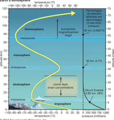
The troposphere, the lowest layer of the atmosphere, extends from the surface to 7-9 km in polar regions and 15-18 km in the tropics. In the troposphere, the temperature decreases with the altitude. A rising air parcel adiabatically cools down as it expands at lower pressure. The variation of temperature with the altitude, referred as adiabatic lapse rate, is rather regular but depends on the air moisture. It ranges from -3 K km−1 in wet condition to -10 K km−1 in dry
condition. The troposphere contains about 75 % of the atmosphere’s total mass and 99 % of its water vapor. It is also the layer in which most of weather-related
phenomena occur because of the turbulent vertical mixing favored by the negative lapse rate. This characteristic earned it its name, derived from the Greek ‘tropos’ for turning (understand mixing). The top of this layer, where the temperature reaches its minimum, is referred as tropopause and marks the transition between the troposphere and the upper layer, the stratosphere.
The stratosphere extends over 40 km and it is characterized by a positive lapse rate, increasing from 1 K km−1 in its lower end to 3 K km−1 in its upper end. The
rise of temperature with the altitude is caused by the large O3 content, the ozone
layer, which absorbs the solar ultra violet (UV) radiation and converts it into heat. With higher temperature in the upper part of this layer, a rising air parcel cooled by its adiabatic expansion becomes colder than its environment and is inclined to return to its equilibrium level. This limits the vertical mixing in the stratosphere and results in an horizontal stratification. The name stratosphere finds its origin in the Latin ‘stratus’ and French ‘sph`ere’, literally meaning a sphere of layers. The temperature reaches its maximum at the stratopause at about 50 km, which marks the transition level to the next layer, the mesosphere.
Figure 1.1: Schematic representation of the atmospheric layers with the profile of temperature (yellow, left) and pressure (black, right). Credit: Encyclopædia Britannica 2012.
de-crease in temperature with the altitude up to the mesopause at about 80 km. Above, lies the thermosphere (from the Greek ‘thermos’ for hot) up to about 600 km and the exosphere (from the Greek ‘exo’ for outer side) that does not really have an upper limit as it progressively fades into space. Both layers are marked by the increase of temperature with the altitude due to the molecular oxygen absorption of high energetic solar UV radiation. Molecules and atoms at these levels are ionized by the UV light so that these layers can also be referred as ionosphere. The temperature in these levels can reaches several thousands of degrees, but because of the low density, it cannot be ‘felt’ as the temperature in a dense medium and only have a meaning in physical applications. Figure 1.1 schematically summarizes the different atmospheric layers as well as the profile of temperature and pressure.
Finally, since the exosphere does not have an outer border, we can wonder where the limit between the atmosphere and space is. This limit was first offi-cially defined by the National Advisory Committee for Aeronautics, the National Aeronautics and Space Administration (NASA) predecessor, as the altitude where the atmospheric pressure was less than one pound per square foot. It corresponds to the altitude (∼50 miles – 81 km) where airplane control surfaces (the moving parts of the wings and tail) can no longer be used. This limit is still used by the US Air Force awarding astronaut wings to pilots flying beyond 50 miles. NASA however, uses today the 62 miles - 100 km Karman limit, defined as the altitude where suborbital speed (from 950 m s−1) are required to be reached.
1.2
Atmospheric circulation
The combined effect of the meridional thermal surface gradient resulting from the solar radiation, the large scale energy transfer conveyed through the water vapor phase changes, and the Earth rotation deflecting equator-ward winds to the west and pole-ward winds to the east, drives the general circulation features observed in the atmosphere. The troposphere is divided in three wind cells (by hemisphere): the Hadley, the Ferrel, and the Polar cells preventing a direct circulation from pole to equator.
Hadley cells, the largest ones, are situated each side of the equator. The warm equatorial surface gives rise to warm and moist air up-welling, producing cloud and atmospheric instability, which results in a band of low pressure at the equator. The release of latent heat when atmospheric water vapor condenses further enhances the cell circulation. At the tropopause, the air flows pole-ward, experiencing drying and cooling as the water vapor condensates or sublimates, and sinks between 30 and 40◦ latitude in both hemispheres. A part of the sinking air returns toward the
effect) and rises again in a new cycle. The low pressure band where the bottom winds of the Hadley cells converge is referred as Inter Tropical Convergence Zone (ITCZ) and is associated with abundant precipitations in all seasons. Owing to the Earth’s axis tilt, the ITCZ shifts north and south of the equator in the summer hemisphere where the incoming solar radiation is the largest.
The middle cells, known as Ferrel cells, are characterized by low level air flowing pole-ward in westerly winds and rising at the pole front where the warm mid-latitude air meets the cool polar air at 60-70◦ latitude in both hemispheres. The
rising air generates moderate precipitations in all seasons at these latitudes. At the top of the troposphere, the circulation entrains the air back to low latitudes, where it joins the sinking air of the Hadley descending branch. Sinking air results in high pressure zones predominantly dry and cloud free. Most of the deserts are found near these latitudes.
Finally, the Polar cells, which are the smallest, cover the polar latitudes. Rising air at the polar front sinks at the pole and flows back to lower latitudes at the surface with easterly winds. Figure 1.2 schematically summarizes these different circulation features.
Figure 1.2: Schematic representation of atmospheric cells and wind patterns (Lut-gens et al., 2001).
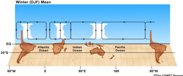
In the tropics, another circulation pattern featuring rising and sinking motion also occurs along with the Hadley cell, but in the east-west direction. This sec-ondary circulation, known as Walker circulation, results from zonal gradient in surface temperature, linked to oceanic thermal structure and continental radia-tive heating. The warm western Pacific as well as the tropical Africa and South
America are regions of rising motion of air in the summer, when the solar radi-ation is maximum. This pattern is also enhanced by the latent heat released by strong thunderstorm activity associated with heavy rainfalls. Lofted air preferen-tially sinks in eastern Pacific and Atlantic, and western Indian Ocean. Figure 1.3 depicts the rising and sinking motion of the Walker circulation over the southern tropics in summer.
Figure 1.3: Schematic representation of the Walker circulation patterns in the southern hemisphere in summer. Credit: COMET Program of the UCAR (http: //meted.ucar.edu/).
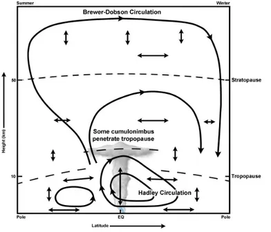
In contrast to the troposphere, a global circulation in which tropospheric air enters the stratosphere in the tropics and moves upward and poleward before de-scending in middle and high latitudes was brought to light by Dobson et al. (1929) and Brewer (1949). The term ‘Brewer-Dobson circulation’ is used for the first time by Newel (1963) to define this circulation. This circulation features a per-sistent poleward mass flow in the middle and upper winter stratosphere driven by an extratropical Rossby wave pump (Plumb, 2002). The pumping results from a non-local effect of the wave drag, which originates from the dispersion of up-ward propagating waves from the troposphere. The planetary-scale Rossby wave westward drag has a pumping action that drives the air poleward to conserve the angular momentum. This wave driven mechanism pulls up the air from the tropics and pushes it down at higher latitudes. The Brewer-Dobson circulation extends up to the mesosphere where the mass transport is from the summer to the winter pole. The mesospheric wave pumping results from buoyancy and gravity waves causing an eastward drag/equatorward pumping in summer and westward drag/poleward pumping in the winter hemisphere. A comprehensive review of the Brewer-Dobson
circulation was recently conducted by Butchart (2014). Figure 1.4 schematically illustrates the Brewer-Dobson circulation.
Figure 1.4: Schematic representation of the meridional Brewer-Dobson circulation in the stratosphere and mesosphere. Credit: COMET Program of the UCAR (http://meted.ucar.edu/) and WMO (1985).
1.3
Moisture in the atmosphere
Water vapor not only affects the atmosphere circulation through the release of latent heat, the cloud formation, and the global distribution of precipitation, but it is also the predominant natural greenhouse gas in the atmosphere. Both obser-vations and models show an increase of tropospheric H2O with the rise of global
temperature (Soden et al., 2005; Dessler, 2013) that results in further warming as H2O feedback was shown to double the warming caused by CO2 alone (Hall
and Manabe, 1999; Held and Soden, 2000). In the stratosphere, H2O exerts an
influence on both the Earth’s energy budget by absorbing solar down-welling and planetary up-welling radiations, and on the ozone chemistry as one of the main sources of hydroxyl radical (OH), thus having a significant feedback contributing to climate changes (Solomon et al., 2010; Dessler et al., 2013). To understand these mechanisms, some key water fundamentals are reviewed below.
1.3.1
Saturation and phase changes
The saturation vapor pressure is the limit beyond which atmospheric H2O
con-denses (or deposits) to form droplets (or ice crystals). Thus, it indicates how much water vapor can be held in the atmosphere. The partial pressure of H2O, referred
as water pressure (e) controls the rate at which H2O condenses or deposits and is
defined by the perfect gas law:
e = ρνRνT (1.1)
where ρν is the H2O mass per unit volume, Rν the gas constant for water, and
T the temperature. When this rate is in balance with the rate of evaporation or
sublimation, then the pressure is said to be saturated and the saturated vapor pressure (es) follows the Clausius-Clapeyron equation:
des
dT = esL
RνT
(1.2) where L is the latent heat of vaporization or sublimation. Assuming a constant L, eq. 1.2 can be integrated as follows:
es= A exp(
−L
RνT) (1.3)
with A an integration constant (Sherwood et al., 2010; Koutsoyiannis et al., 2012). Note that the relative humidity can be expressed as the simple ratio e/es.
Figure 1.5: Representation of the exponential rise of saturation vapor pressure with the rise of temperature. Credit: Julander, University of Utah (http://www. civil.utah.edu/˜cv5450/atmosphere/atmos.html)
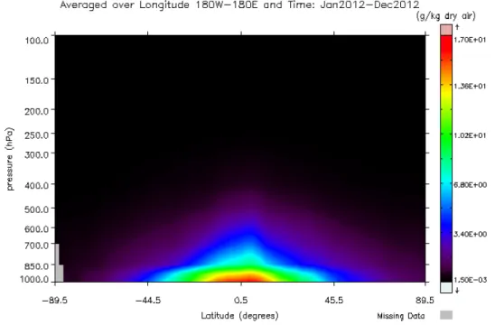
The saturation vapor pressure is thus an exponential function of the tempera-ture (see Fig. 1.5), meaning that warmer air can hold more moisture. As temper-ature decreases with altitude in the troposphere, so does es. It results that most
of H2O is found in the lower end of the troposphere and in the equatorial region,
as shown on Fig. 1.6. The moisture of an air parcel in supersaturation condi-tion will condense to remove the excess of water vapor and return to equilibrium, i.e. the saturation level. Conversely, droplets (or ice crystals) in sub-saturated air will evaporate (or sublimate) to reach the saturation. Over liquid, supersatura-tion reaches at most 1-2 % because the nuclei that serve as basis for the vapor to condensate (mostly inorganic salts) are abundant in the troposphere. At low temperature, freezing results from homogeneous and heterogeneous nucleation. In homogeneous nucleation, liquid droplets spontaneously freeze, but it requires tem-perature down to -35◦C. Ice nuclei able to initiate ice in heterogeneous nucleation
also exist but, insoluble and hexagonal shaped, are rare in the atmosphere (Har-rison, 2000; Pruppacher and Klett, 2010). It results that supersaturation over ice commonly rises to 10-30 %.
Figure 1.6: Tropospheric H2O mass mixing ratio (g kg−1 dry air) from 89.5◦S to
89.5◦N averaged over all longitudes in 2012, from AIRS global monthly level-3
1.3.2
Tropospheric water vapor
The main sources of tropospheric H2O are the evaporation from ocean, which is
estimated to 425 × 103km3yr−1, and the continental evapotranspiration
account-ing for 71 × 103km3yr−1 (Delmas et al., 2005). Additional H
2O also originates
from anthropogenic activities through irrigation, power plant cooling, and fos-sil fuel combustion (the combustion of methane for example: CH4 + 2 O2 −−→
CO2 + 2 H2O + energy). Nonetheless, these anthropogenic emissions represent
less than 1 % of the total sources and have a negligible impact on the H2O
bud-get (IPCC, 2007). Also, H2O does not accumulate in the troposphere like other
greenhouse gases, but condenses and precipitates within about 10 days. For this reasons, tropospheric H2O is not considered as a forcing of climate change, but
rather a feedback agent. As seen in the previous section, the atmospheric moisture, and thus its feedback, depend on temperature. Hence, observations show that the 3.5 % rise of tropospheric H2O since the 1970s is consistent with the 0.5◦C global
warming over the same period (IPCC, 2013). The resulting feedback, expressed as the rate of energy transferred per unit of surface and per unit of temperature, is 1.98±0.21 W m−2K−1 (Held and Shell, 2012).
1.3.3
Stratospheric water vapor
In the stratosphere, H2O also affects the temperature as it participates to the
warming of the troposphere and the cooling of the stratosphere (Solomon, 2010). Furthermore, as one of the main source of hydroxyl radical through photodis-sociation (H2O + hν −−→ H + OH) and reactions with excited oxygen atoms
(H2O + O(
1D) −−→ 2 OH), water vapor participates to the stratospheric ozone
de-pletion (Stenke and Grewe, 2005). Zonldo et al. (2000) also underlined the key role of stratospheric H2O in the formation of Polar Stratospheric Clouds (PSCs) which
lead to the activation of the ozone-destroying form of chlorine. H2O in the
strato-sphere has two distinct sources. The first and main source has a dynamical nature as H2O is transported from the troposphere, where it is found in abundance, to the
stratosphere. We can differentiate: i) a slow large-scale transport characterized by the radiative lofting of moisture-rich air parcels that are strongly dehydrated before to enter the stratosphere when they cross the very cold tropopause region, and ii) a fast local transport characterized by the convective injection of water (mainly ice crystals) directly into the lower stratosphere. Stratospheric entry is estimated to be on average ∼3 ppmv. Troposphere-to-stratosphere transport pro-cesses and their implication for the water vapor budget are further discussed in the next chapter. The second source of H2O in the stratosphere is the oxidation of
methane by the hydroxyl radical (CH4+ OH −−→ CH3+ H2O). Oxidation of the
results in production of H2O but preferentially happens in the upper stratosphere
(Le Texier, 1988).
Natural sources of CH4 are the release from geological deposits and natural
gas resulting from anaerobic reaction in wetland. Anthropogenic emissions have however become increasingly important since the industrial era and now account for more than half of the total emissions. The CH4concentration in the atmosphere
is 2.5 time higher today than at the beginning of the XIXth century (IPCC, 2013).
This is due to the increase of livestock farming, expansion of rice paddy cultivation, fermentation of organic waste in landfill, and fossil fuel extraction and combustion. Nonetheless, rise in CH4 concentration can only account for one third of the recent
(1980-2010) increase of stratospheric H2O (27±6 %) (Rohs et al., 2006; Hurst et
al., 2011). Changes in tropical tropopause temperature controlling the H2O entry
into the stratosphere also drive its variability but the lack of long-term datasets makes interpretations difficult. Hegglin et al. (2014) recently proposed an approach to merge multiple satellite datasets, which resulted in a stratospheric H2O record
extending back to 1988. Nonetheless, the contribution of mechanisms driving the variability and distribution of H2O in the stratosphere is still debated and poorly
represented in global models, although stratospheric H2O was shown to have a
significant climate feedback (potentially up to 0.3 W m−2K−1 according to Dessler
et al. (2013)).
1.4
Carbon in the atmosphere
The Earth is composed of several carbon reservoirs that communicate through flux exchanges at different time scales. The time scale for the exchanges of carbon con-tained in the atmosphere, the oceans, the biosphere, soils and freshwater ranges from the year to the millennium. Although it can seem long periods, these ex-changes are considered fast with respect to those occurring in geological reservoir like rocks and sediments (the most abundant reservoirs of carbon, see Fig. 1.7), which require time scales greater than 10000 years to interact with the other reser-voirs through processes such as volcanism or chemical weathering and erosion.
Focusing on the atmosphere, the dominant carbonic compounds are carbon dioxide (CO2), with a mass estimated to 828 Petagrams of Carbon (PgC), methane
(CH4), with 3.7 PgC and carbon monoxide (CO), with 0.2 PgC (Joos et al, 2013;
IPCC, 2013). Carbon is also found in small quantity in hydrocarbons, black car-bons, and volatile organic compounds (VOCs).
1.4.1
Atmospheric carbon monoxide
In the following sections, we will emphasis the CO characteristics as it is an im-portant atmospheric pollutant impacting air quality and climate change.
Sources and sinks
CO is both emitted at the surface and produced in the atmosphere, but because of its short lifetime of about 2 months, it is not a well-mixed trace gas. Its abundance presents large gradients (horizontal and vertical) with mixing ratios of a few tens of part per billion in volume (ppbv) far from its sources like in remote southern ocean, to more than 1 part per million in volume (ppmv) in highly polluted areas (Novelli, 1998).
Figure 1.7: Schematic representation of the carbon reservoirs and fluxes driving the carbon cycle. Reservoirs and their carbon mass (in gigaton of carbon) are shown in white. Arrows represent the fluxes between reservoirs. The exchange processes and flow rate are shown in yellow (in gigaton per year). In red is rep-resented the anthropogenic add up on natural cycle. Credit: Office of Biological and Environmental Research of the U.S. Department of Energy Office of Science. At the surface, CO is mainly released from the incomplete combustion of biomass, biofuel, and fossil fuel. An example is the incomplete combustion of
CH4 that occurs when the supply of oxygen is poor and produces carbon
monox-ide instead of carbon dioxmonox-ide as shown below: CH4+ 2 O2 −−→CO2+ 2 H2O (complete)
2 CH4+ 3 O2 −−→2 CO + 4H2O (incomplete)
Incomplete combustion represents about 1640±800 Teragrams of carbon monoxide (TgCO) per year according to Delmas et al. (2005). Emissions from oceans and biosphere also add a small contribution to the total amount (192±130 TgCO yr−1).
In the troposphere, CO results from the oxidation of VOCs and hydrocarbons by the radical OH. Although the oxidation of isoprene (C5H8) has a significant
con-tribution to CO production with ∼330 TgCO yr−1, the main atmospheric source is
the oxidation of CH4, which represents ∼690 TgCO yr−1 (Pfister et al., 2008). The
oxidation of CH4 is described below:
First, CH4 reacts with OH to form methyl radical (CH3).
CH4+ OH −−→ CH3+ H2O (1.4)
A sequence of reactions involving CH3and the by-products methyl peroxide (CH3O2),
methyl hydroperoxy (CH3OOH), and methyl oxide (CH3O) results in the
produc-tion of formaldehyde (HCHO).
CH3+ O2+ M −−→ CH3O2 + M (1.5)
CH3O2+ NO −−→ CH3O + NO2 (1.6)
CH3O2+ HO2 −−→CH3OOH + O2 (1.7)
CH3OOH + hν −−→ CH3O + OH (1.8)
CH3O + O2 −−→HCHO + HO2 (1.9)
Finally, HCHO can form CO by photodissociation or through its photodissociation or oxidation in an aldehyde compound (HCO).
HCHO + hν −−→ CO + H2 (1.10)
HCHO + OH −−→ HCO + H2O (1.11)
HCHO + hν −−→ HCO + H (1.12)
Along with these reactions, the main atmospheric sink of CO is its own oxida-tion by the OH radical, which represents a removal of about 2000±750 TgCO yr−1
(Delmas et al., 2005).
CO + OH −−→ CO2+ H (1.14)
This reaction also represents consequently a sink for OH. The CO oxidation is not constant throughout the year and presents a seasonal variability linked to the abundance of OH radical in the atmosphere. In the summer hemisphere, the photodissociation of O3produces excited oxygen atoms which can react with water
molecules to form OH radical. O3+ hν −−→ O(
1D) + O
2 (1.15)
O(1D) + H
2O −−→ 2 OH (1.16)
The increase of OH results in a larger removal of CO and then, in its lower abun-dance in summer.
The interaction of CO with OH also perturbs the oxidation of other trace gases. Taking the example of O3 (vital in the stratosphere to stop the UV radiation, but
a health threatening pollutant in the troposphere), the oxidation of CO can either favor the depletion of O3 or on the contrary participate to its production. This
depends on the atmospheric abundance of nitric oxide (NO) and nitrogen dioxide (NO2), referred as NOx, in the region where CO is emitted or transported. The
oxidation of CO participates to the reduction of O3 when NOx are not abundant
and do not participate to the reaction.
CO + OH −−→ CO2+ H (1.17)
H + O2+ M −−→ HO2+ M (1.18)
HO2+ O3 −−→ OH + 2 O2 (1.19)
So that the net reaction is:
CO + O3 −−→CO2+ O2 (1.20)
However, if the region is rich in NOx, then HO2 catalyzes the reaction to form O3
CO + OH −−→ CO2+ H (1.21)
H + O2+ M −−→ HO2+ M (1.22)
HO2+ NO −−→ NO2+ OH (1.23)
NO2+ hν −−→ NO + O (1.24)
O + O2+ M −−→ O3+ M (1.25)
So that the net reaction is:
CO + 2O2 −−→O3+ CO2 (1.26)
In summary, according to Thomas and Devasthales (2014), an increase in CO content in the atmosphere would not only add more CO2 as seen in reactions 1.20
and1.26, but because CO is a sink of OH radical, it would also indirectly increase the levels of O3 and CH4, then subject to a lesser removal from the OH radical.
1.4.2
Impact of CO on climate
According to the last IPCC report (2013), the radiative forcing resulting from the CO atmospheric drivers (CO2, CH4, and O3) is 0.23±0.07 W m−2 or about
10 % of the total anthropogenic radiative forcing relative to 1750 estimated to 2.29±1.04 W m−2. Although less than the direct forcing caused by CO
2(1.68±0.35 W m−2)
and CH4 (0.97±0.23 W m−2), CO has (indirectly) the third largest impact among
the trace gases on the atmospheric radiative balance.
Nonetheless, several studies (Yurganov et al., 2010; Fortems-Cheiney et al., 2011; Worden et al., 2013; Warner et al., 2013; He et al., 2013), based on satel-lite observations, highlighted a global decrease in tropospheric CO over the last decade. More specifically, Worden et al. (2013) analyzed the trend of CO (total column) in the datasets of four instruments: the Measurement of Pollutants in the Troposphere (MOPITT), the Atmospheric InfraRed Sounder (AIRS), the Tro-pospheric Emission Spectrometer (TES), and the Infrared Atmospheric Sounding Interferometer (IASI). They showed that CO decreased over the last decade in both hemispheres, although to a greater rate in the northern hemisphere (∼1 % yr−1).
The decreasing trends are even more accentuated over highly populated regions such as China (-1.6 % yr−1), Europe (-1.4 % yr−1), or USA (-1.4 % yr−1). The
de-creasing trend in CO agrees with the finding presented in this dissertation and will be further discussed, along with the tropospheric CO variability, in chapter 4.
Chapter 2
Water vapor monitoring in the
tropical tropopause layer from
space-borne observations
2.1
General introduction
Tropospheric water vapor accounts for more than half of the Earth greenhouse effect and is now recognized as a critical component of climate change. Predicted by global climate models, this strong water vapor feedback has been confirmed after a decade of AIRS tropospheric H2O observations. Anthropogenic emissions
of greenhouse gases lead to a rise in temperature. A warmer atmosphere can absorb more H2O and more H2O results in further warming. It is a spiraling cycle.
In the stratosphere, H2O undergoes chemical reactions that contribute to the
ozone depletion. Furthermore, recent evidence has been reported that strato-spheric H2O also has a significant climatic feedback. However, unlike in the
tropo-sphere, the mechanisms at the origin of the stratospheric H2O variability are still
poorly understood and highly debated. With the CH4 oxidation, the transport
from the troposphere (primarily occurring in the tropics) is the principal source of stratospheric H2O. Slow radiative ascent and fast convective lofting are the
compet-ing mechanisms of the troposphere-to-stratosphere transport. Although the slow advection is known to dehydrate the air parcels entering the stratosphere, convec-tive uplift can either result in hydration or dehydration of the tropical tropopause layer and the lowermost stratosphere.
The TRO-pico project, named after the Pico-SDLA hygrometer, is a French National Research Agency (ANR) funded field experiment aiming to study the contribution of deep tropical convection to the H2O abundance in the TTL and
ob-servations coupled with model simulations, the project is expected to deliver a comprehensive analysis of local scale H2O variability. It will be further detailed in
chapter 3.
In this chapter, I present a study that I led on the implication of daytime and night-time difference of the Microwave Limb Sounder (MLS) H2O, cloud Ice Water
Content (IWC), and temperature measurements in the tropical tropopause layer (TTL). I analyzed 8 years of MLS observations in the tropical band (25◦N-25◦S)
and over restricted areas of north and south tropical South America, Africa, mar-itime continent and western Pacific to emphasize the different convective charac-teristics over land versus ocean. To better focus on the seasonal cycle of convection, semi-annual and inter-annual variability were removed by filtering their contribu-tion in the signal. We investigated several hypotheses on the possible nature of dynamical and physical processes driving the observed variability. The analysis of the most convective days shows an impact of the continental convection in the TTL, not observed in oceanic areas. Anomalies of H2O, IWC and temperature
calculated for daytime and night-time separately reveal the hydrating nature of this process. This study offers a climatological baseline to help interpret results from TRO-pico with respect to larger scales as well as future research related to the tropical convection and its impact on H2O.
This chapter is based on “Carminati, F., Ricaud, P., Pommereau, J.-P., Rivi`ere,
E., Khaykin, S., Atti´e, J.-L., and Warner, J.: Impact of tropical land convection on the water vapour budget in the tropical tropopause layer, Atmos. Chem. Phys., 14, 6195-6211, doi:10.5194/acp-14-6195-2014, 2014” (http://www.atmos-chem-phys. net/14/6195/2014/acp-14-6195-2014.html). Text, figures and tables are
iden-tical to the original article, however the page setup was modified in order to ease the reading. References are in the ‘Bibliography’.
2.2
Article 1 - Impact of tropical land convection
on the water vapour budget in the tropical
tropopause layer
Abstract
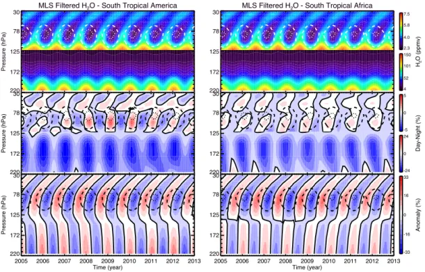
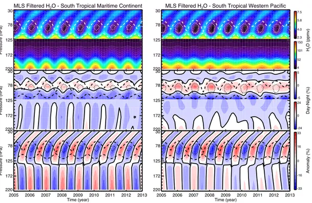
The tropical deep overshooting convection is known to be most intense above conti-nental areas such as South America, Africa, and the maritime continent. However, its impact on the tropical tropopause layer (TTL) at global scale remains debated. In our analysis, we use the 8-year Microwave Limb Sounder (MLS) water vapour (H2O), cloud ice-water content (IWC), and temperature data sets from 2005 to
water vapour variability in the TTL, and separately in the northern and south-ern tropics. In the tropical upper troposphere (177 hPa), continents, including the maritime continent, present the night-time (01:30 local time, LT) peak in the water vapour mixing ratio characteristic of the H2O diurnal cycle above tropical land.
The western Pacific region, governed by the tropical oceanic diurnal cycle, has a daytime maximum (13:30 LT). In the TTL (100 hPa) and tropical lower strato-sphere (56 hPa), South America and Africa differ from the maritime continent and western Pacific displaying a daytime maximum of H2O. In addition, the relative
amplitude between day and night is found to be systematically higher by 5–10 % in the southern tropical upper troposphere and 1–3 % in the TTL than in the north-ern tropics during their respective summer, indicative of a larger impact of the convection on H2O in the southern tropics. Using a regional-scale approach, we
investigate how mechanisms linked to the H2O variability differ in function of the
geography. In summary, the MLS water vapour and cloud ice-water observations demonstrate a clear contribution to the TTL moistening by ice crystals overshoot-ing over tropical land regions. The process is found to be much more effective in the southern tropics. Deep convection is responsible for the diurnal temperature variability in the same geographical areas in the lowermost stratosphere, which in turn drives the variability of H2O.
2.2.1
Introduction
The tropical tropopause layer (TTL), the transition layer sharing upper tropo-spheric (UT) and lower stratotropo-spheric (LS) characteristics, is the gateway for tro-posphere to stratosphere transport (TST), and plays a key role in the global com-position and circulation of the stratosphere (Holton et al., 1995; Fueglistaler et al., 2009). TST processes responsible for the upward motion of air masses impact-ing on the water budget are (1) the slow ascent (300 m month−1) due to radiative
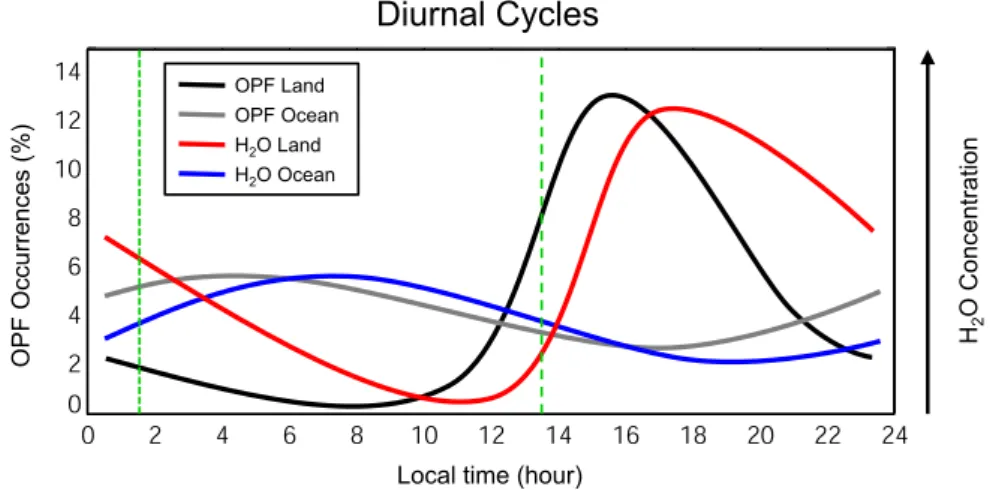
heating associated with horizontal advection, known as “cold trap” (Holton and Gettelman, 2001; Gettelman et al., 2002; Fueglistaler et al., 2004), (2) fast over-shooting updraughts followed by detrainment referred to as “freeze and dry” pro-cess (Brewer, 1949; Sherwood and Dessler, 2000, 2001, 2003; Dessler, 2002), and (3) the fast and direct injection by “geyser-like” overshoots (Knollenberg et al., 1993; Corti et al., 2008; Khaykin et al., 2009) that can penetrate into the LS. The long-known convective area in the western Pacific, referred to as “stratospheric fountain” (Newell and Gould-Stewart, 1981), has been the focus of numerous field campaigns. However, studies in the early 2000s pointed out that most vigorous convections occur over continental tropical areas where overshooting precipitation features (OPFs) are more frequent (Alcala and Dessler, 2002; Liu and Zipser, 2005). These convective activities show a marked diurnal cycle with a pronounced late afternoon maximum (Liu and Zipser, 2005) in contrast to oceanic regions
of little diurnal variation. Evidence of TTL-penetrating overshooting continental convection and its impact on trace gases, aerosols, water vapour, ice particles, chemical composition, and transport mechanisms were gathered during the Hibis-cus, Stratospheric-Climate Links with Emphasis on the Upper Troposphere and Lower Stratosphere – Ozone (SCOUT-O3), SCOUT – African Monsoon and Mul-tidisciplinary Analyses (AMMA) and Tropical Convection, Cirrus, and Nitrogen Oxides Experiment (TROCCINOX) field campaigns in South America, western Africa and Australia between 2001 and 2006 (Corti et al., 2008; Schiller et al., 2009; Cairo et al., 2010; Pommereau et al., 2011). A significant contribution of continental convection to the chemical composition of the LS has been reported by Ricaud et al. (2007, 2009) from Odin-SMR (sub-millimetre radiometer) satel-lite observations. They showed a higher mixing ratio of tropospheric trace gases (N2O and CH4) in the TTL during the southern summer. The results of Ricaud
et al. (2007, 2009) are consistent with the cleansing of the aerosols in the LS seen by Cloud-Aerosol Lidar and Infrared Pathfinder Satellite Observation (CALIPSO) during the same season (Vernier et al., 2011).
The present study addresses one of the most debated aspects of the TTL and the LS, the budget of water vapour (H2O), and aspires to be a baseline for
fur-ther studies related to the TRO-pico project (www.univ-reims.fr/TRO-pico).
TRO-pico aims to monitor H2O variations in the TTL and the LS linked to deep
overshooting convection during field campaigns, which took place in the austral summer in Bauru, Sao Paulo state, Brazil, involving a combination of balloon-borne, ground-based and spaceborne observations and modelling.
Being the most powerful greenhouse gas and playing an important role in the UT, TTL and LS chemistry as one of the main sources of OH radicals, H2O is
a key parameter in the radiative balance and chemistry of the stratosphere and its variation can affect climate (Solomon et al., 2010). The mean tropical (20◦N–
20◦S) H
2O mixing ratio is estimated to be between 3.5 and 4 ppmv (parts per
million by volume) in the TTL at 100 hPa (Russell III et al., 1993; Weinstock et al., 1995; Read et al., 2004; Fueglistaler et al., 2009). In agreement with this mean mixing ratio, Liang et al. (2011) estimated a mean H2O stratospheric entry
of 3.9 ± 0.3 ppmv at 100 hPa in the tropics.
The moistening of the lower stratosphere by convective overshooting is a well demonstrated process, nonetheless, its contribution at global scale is still debated. For example, in 2006, the SCOUT-AMMA campaign in western Africa revealed a 1–3 ppmv (with a 7 ppmv peak) moistening of the 100–80 hPa layer (Khaykin et al., 2009). Although this process is well captured in cloud-resolving models (Chaboureau et al., 2007; Jensen et al., 2007; Grosvenor et al., 2007; Chemel et al., 2009; Liu et al., 2010; Hassim and Lane, 2010), global-scale models do not yet integrate this sub-grid-scale non-hydrostatic process, which may result in an