Michel : Assistant Professor of Finance, HEC Montréal and CIRPÉE. Phone : 514 340-7153; Fax : 514 340-5632
jean-sebastien.michel@hec.ca
Cahier de recherche/Working Paper 13-19
Investor Overreaction to Analyst Reference Points
Jean-Sébastien Michel
Abstract:
In this paper, I document analysts’ reliance on the company issued guidance range as a frame of reference in making their EPS forecasts. Analysts who use the guidance range as a reference may limit information diffusion to market participants by keeping their true beliefs private. I therefore analyze the stock market’s reaction to analyst forecasting decisions, and find that investors overreact to forecasts that are exactly equal to the minimum or maximum of the guidance range, but do not overreact to other types of forecasts. The evidence presented is most consistent with overreaction driven by overconfident investors who trade too much in the face of information uncertainty.
Keywords: Overreaction, Stock Returns, Reference Point, Analyst Earnings Forecasts
1
Introduction
In this paper, I document that analysts use the company issued
guid-ance range as a reference when forecasting the firm’s earnings per share
(EPS). In the week following company issued EPS guidance, over one
third of analyst forecasts are that are exactly equal to the minimum or
maximum of the guidance range. Analyst forecasts within the guidance
range (including the endpoints) are less biased and more accurate than
forecasts outside of the guidance range. Indeed, if staying within the
reference range is beneficial to analysts in terms of their reputation, why
don’t all analysts do it? I find that analysts’ decision to forecast
out-side of the guidance range is related to analysts’ experience and skill.
Analysts with less experience or less skill are more likely to exceed the
guidance range than analysts with more experience or more skill.
While using the guidance range as a reference is advantageous to
ana-lysts, it also suggests that in the absence of company issued guidance, an
analyst whose forecast equals the guidance range minimum (maximum)
would have provided an even lower (higher) EPS forecast. As such,
the reference range may limit information diffusion to market partici-pants. I therefore analyze the stock market reaction to analyst
forecast-ing decisions, and find that investors overreact to analyst forecasts that
are exactly equal to the minimum or maximum of the company issued
guidance range. This result is not due to the magnitude of the forecast;
those that exceed the guidance range endpoints, the overreaction is even
more pronounced.
Investors’ overreaction in the face of reference point induced
infor-mation uncertainty may be due to overconfidence as in Odean (1998,
1999). Consistent with this explanation, I find that there is excessive
share turnover when forecasts are exactly equal to the guidance range
endpoints are given. Again, this is not due to the magnitude of the
fore-cast since I also find excessive share turnover for forefore-casts equal to the
guidance range endpoints relative to forecasts that exceed the guidance
range endpoints. Importantly, when there are analyst forecasts that equal
both the minimum and maximum of the company issued guidance range
on the same day, firms experience the largest amount of share turnover,
but no reliably abnormal stock market returns. This suggests that in
situ-ations where information uncertainty is at its highest, investor
overconfi-dence is also at its highest, but the overreaction to forecasts equal to the
minimum of the company issued guidance is offset by the overreaction to forecasts equal to the maximum.
Recent papers have documented the impact of reference points when
making important investing and financing decisions. Baker, Pan, and
Wurgler (2012) find that higher recent peak prices are associated with a
higher offer premium and a higher likelihood of deal success in mergers and acquisitions. Loughran and Ritter (2002) propose a prospect theory
explanation for why issuers leave money on the table in initial public
relative to the midpoint of the file range; a reference point that
execu-tives of the issuing firm have anchored on. Ljungqvist and Wilhelm Jr.
(2005) further show that chief executive officers of recent IPO firms make subsequent decisions consistent with a reference point measure
of their perception of the IPOs outcome. Dougal, Engelberg, Parsons,
and Van Wesep (2012) document that the path of credit spreads since
a firm’s last loan influences the level at which it can currently borrow.
The authors attribute this finding to anchoring on past deal terms.
Refer-ence points have even been found to impact sell-side analysts. Campbell
and Sharpe (2009) find that consensus forecasts of monthly economic
releases are systematically biased toward the value of previous months’
releases, consistent with an anchoring and adjustment heuristic. Cen,
Hilary, and Wei (2013) document that analysts make optimistic
(pes-simistic) forecasts when a firm’s forecasted EPS is lower (higher) than
the industry median, consistent with the idea that analysts anchor on the
industry norm. This paper contributes to this literature by documenting
for the first time analysts’ reliance on the company issued guidance range
as a frame of reference in making their EPS forecasts. This literature is
largely based on the works of Tversky and Kahneman (1974) and
Kahne-man and Tversky (1979), which document several experimental results
where individuals do not act in accordance with expected utility
the-ory. To account for individuals’ decision making under risk, Kahneman
and Tversky (1979) develops a prospect theory whereby individuals
instead of final asset positions. The reference point in their theory is
derived from the context at hand.1
This paper also contributes to the literature on the overreaction of
stock prices to various events. Empirically, a number of papers have
found that returns are negatively autocorrelated over a 3-5 year
hori-zon in various markets (e.g. Fama and French, 1988; Poterba and
Sum-mers, 1988; Cutler, Poterba, and SumSum-mers, 1991). De Bondt and Thaler
(1985, 1987) find that portfolios of stocks with extremely poor returns
over the previous five years dramatically outperform portfolios of stocks
with extremely high returns, even after making the standard risk
adjust-ments. La Porta (1996) finds that stocks with the highest growth
fore-casts earn much lower future returns than stocks with the lowest growth
forecasts. Moreover, on average, stocks with high growth forecasts earn
negative returns when they subsequently announce earnings. La Porta,
Lakonishok, Shleifer, and Vishny (1997) find that glamour stocks also
earn negative returns on the days of their future earnings announcements,
and value stocks earn positive returns. Lakonishok, Shleifer, and Vishny
(1994) find large differences between the returns of extreme value and glamour deciles. Chopra, Lakonishok, and Ritter (1992) find in
portfo-lios formed on prior five-year returns that past losers outperform past
1The terms "reference point" and "anchor point" are generally used synonymously in the finance
litera-ture. However, Kahneman (1992) draws a sharp distinction between the two terms. The author notes that the term "reference point" denotes salient neutral points on evaluation scales, at which the slope of the value function shows an sharp transition, in contrast to the effects of anchors, which are graded. I therefore use the term "reference point" throughout this paper to denote the minimum or maximum of the company issued guidance range, which should indeed be a salient neutral point on the EPS evaluation scale where there are sharp transitions in analysts’ value function.
winners during the subsequent five years. Moreover, the authors find
overreaction for short windows around quarterly earnings announcements.
All of this evidence is consistent with stock market overreaction. Several
models have been proposed to explain the overreaction phenomenon.
Bar-beris, Shleifer, and Vishny (1998) develop a model of investor
senti-ment which is consistent with overreaction of stock prices to a series
of good or bad news. Hong and Stein (1999) model a market populated
by news watchers and momentum traders. If information diffuses grad-ually across investors and momentum traders only implement simple
strategies, then the overall effect is for investors to overreact to stock prices. In the Daniel, Hirshleifer, and Subrahmanyam (1998) model,
overconfident and informed investors overweight their private signal,
causing the stock price to overreact. Furthermore, Ko and Huang (2007)
find in their model that the degree of overreaction in prices is
increas-ing in overconfidence. Overconfidence is also associated with greater
trading volume. Odean (1998) finds that trading volume increases when
price takers, insiders, or market-makers are overconfident. Odean (1999)
and Statman, Thorley, and Vorkink (2006) find that investor
overcon-fidence can explain high observed trading volume. The evidence
pre-sented in this paper is most consistent with overreaction driven by
over-confident investors who trade too much in situations of high information
uncertainty.
The rest of this paper is structured as follows. Section 2 presents the
well as forecasting decisions in the presence of these reference points
are examined in section 3. Investors’ stock market reaction to analyst
reference points is presented in section 4. Conclusions are drawn in
section 5.
2
Research Design and Data
The primary source of data used in this paper is the company issued
EPS guidance from First Call. I only retain range estimates, although
point estimates and qualitative guidance is also available in this dataset.2
I use data on analyst EPS forecasts from the I/B/E/S unadjusted detail dataset, data on standardized unexpected earnings surprises from the
I/B/E/S surprise dataset, and data on realized EPS from the I/B/E/S ac-tual dataset. Returns, prices and shares outstanding are obtained from
CRSP and book values are obtained from Compustat. Finally, the Fama
and French (1993) three factors and the Carhart (1997) momentum
fac-tor are obtained from Professor Kenneth French’s website.3
I examine the data in two different ways throughout this paper. First, I examine analysts’ decision to use the company issued guidance range
as a reference as well as the determinants at that decision. As such,
I merge the I/B/E/S unadjusted detail dataset, which contains individ-ual EPS forecasts for firms being covered by at least one analyst, to the
2It is possible that analysts use the company issued guidance point estimate as a reference, but I do not
explore this possibility since there is no clear prediction with regards to the stock market reaction.
First Call company issued guidance dataset. In order to calculate
fore-cast errors and accuracy, I merge in realized EPS from the I/B/E/S actual dataset. Firm specific data is then merged in to control for company
spe-cific attributes. This sample has 144,566 observations, which represent
individual analyst forecasts of various firms from January 2000 to June
2011.
Second, I examine investors’ reaction to analyst forecasts decisions.
Since multiple analysts sometimes make forecasts for the same firm on
the same day, but daily stock market returns are the same for all of the
an-alysts making these forecasts, I aggregate analyst forecasting decisions
at the firm level. Specifically, I consider a firm’s analysts to have used
the company issued guidance range as a reference if at least one
ana-lyst has provided a forecast equal to the company guidance range low or
high. Using this firm-level measure, I examine the daily factor-adjusted
returns and share turnover surrounding this event, which are merged in
from CRSP. This sample has 45,714 observations, which represent
indi-vidual forecast days of various firms from January 2000 to June 2011.
3
Analyst Forecasting Behavior
This section documents analysts’ tendency to rely on the company
is-sued EPS guidance range as a reference by providing forecasts that
ex-actly equal the minimum or maximum point provided in the guidance.
analyst forecasts relative to the company issued guidance (CIG) range:
(i) Analyst Forecast< CIG Low; (ii) Analyst Forecast = CIG Low; (iii) CIG Low< Analyst Forecast < CIG High; (iv) Analyst Forecast = CIG High; and (v) Analyst Forecast> CIG High. I also examine analysts’ er-rors and accuracy to determine whether the decision to provide a forecast
in a particular category is beneficial. Finally, I examine the determinants
of analysts’ decision to provide forecasts within a particular category.
Figure 1 shows the yearly distribution of forecasts in the above-mentioned
categories, as well as the overall number of forecasts in the sample each
year.4 The figure shows that there is not much variation for each
cate-gory from year to year. In particular, the percentage of forecasts lower
(higher) than the CIG Low (High) hovers at around 5% (15%) over the
sample period, while the percentage of forecasts between the CIG Low
and High hovers around 50%. Similarly, the percentage of forecasts
exactly equal to the CIG Low (High) are around 15% (20%) over the
sample period. However, there are some noticeable trends. The
percent-age of forecasts exactly equal to the CIG Low has become slightly less
prevalent over time, while the percentage of forecasts between the CIG
Low and High has become slightly more prevalent over time. One
possi-ble explanation for this result is that analysts have become slightly more
optimistic over the sample period, although there is no corresponding
increase in the prevalence of analyst forecasts above the CIG High. In
terms of the yearly number of forecasts, the frequency increases in the
4Note that the number of observations in the year 2011 is lower than in any other year because the sample
first four years of the sample, but remains relatively flat thereafter.
The first two columns of table 1 report the frequency and percentage
of forecasts within the afore-mentioned five categories. Surprisingly,
22.06% of forecasts are exactly equal to the maximum of the CIG range.
A further 11.99% of forecasts are exactly equal to the minimum of the
CIG range. 48.31% of analyst forecast can be found within the CIG
end-points. Finally, 6.13% (11.51%) of forecasts are below (above) the
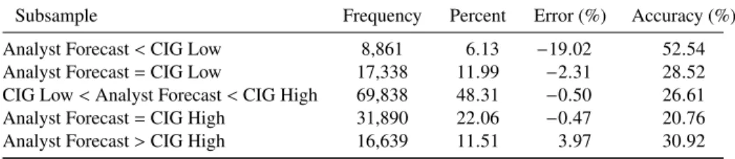
min-imum (maxmin-imum) of the CIG range. Overall, over 80% of forecasts are
within the CIG range and about one third are exactly equal to the
min-imum or maxmin-imum endpoint. These results show that analysts have a
clear preference for providing forecasts within the CIG range. Columns
3 and 4 provide the error and accuracy of these forecasts, respectively.
Analyst error is the percentage difference between the analyst EPS fore-cast and the firm’s realized EPS for the quarterly EPS being forefore-casted,
while analyst accuracy is the absolute value of analyst error. Analyst
errors within the CIG endpoints range from –0.47% to –2.31%.
Ana-lyst forecasts above the CIG maximum are slightly optimistic with an
average error of 3.97%, while forecasts below the CIG minimum are
noticeably pessimistic with an average error of –19.03%. Meanwhile,
analyst unsigned errors within the CIG endpoints range from 20.76%
to 28.52%.5 Forecasts above the CIG maximum are less accurate with
an average unsigned error of 30.92%, while forecasts below the CIG
minimum are even more inaccurate with an average unsigned error of
5Since the accuracy measure is the unsigned error, a higher (lower) number means that the forecast is less
52.54%.
Table 2 reports multivariate regressions of analyst performance on
forecasting categories and firm control variables. Model 1 reports the
impact of the control variables, while in model 2, I add the forecasting
categories to determine their incremental impact. The control variables
are mainly to insure that the impact of forecasting categories on error
and accuracy is not due to known characteristics that make forecasting
EPS difficult, such as past EPS volatility, recent unexpected EPS, firm size and growth, among others. The regression with forecast error as the
dependent variable reveals that providing a forecast below the CIG Low
leads to more pessimistic forecasts than providing a forecast within the
CIG range.6 Similarly, providing a forecast above the CIG High leads
to more optimistic forecasts than providing a forecast within the CIG
range. However, providing a forecast exactly equal to the minimum or
maximum of the CIG range does not lead to any incremental error. This
suggests that, on average, managers providing company issued guidance
are correct in their EPS projections. The regression with accuracy as the
dependent variable shows that providing a forecast below the CIG Low
or above the CIG High lead to more inaccurate forecasts than providing
a forecast within the CIG range. Providing a forecast exactly equal to
the minimum of the CIG range does not lead to any change in accuracy,
while providing a forecast exactly equal to the maximum of the CIG
6This result is not tautological since the ex post realized EPS could be even further below the CIG
range than the analyst forecast, in which case the analyst would be relatively optimistic instead of relatively pessimistic.
range does lead to better accuracy. This may be due to managers’
ten-dency to provide a conservative maximum EPS in order to obtain
posi-tive EPS surprises. Economically, forecasting below the low endpoint of
the CIG range leads to errors that are 14.22 percentage points lower and
accuracy that is 18.48 percentage points higher, while forecasting above
the high endpoint of the CIG range leads to errors that are 3.41
percent-age points higher and accuracy that is 4.58 percentpercent-age points higher. The
economic significance is qualitatively similar to that in table 1.
It is important to note that while providing a forecast outside of the
CIG range is detrimental to analysts on average, since it reduces their
reputation by inducing to more bias and more inaccuracy, it may still be
worthwhile for some analysts to engage in this behavior. In particular,
inexperienced analysts with no track record or analysts that have
per-formed poorly in the past may feel that they need to make bold forecasts
as in Clement and Tse (2005) in order to establish or reestablish their
reputation. We explore this possibility in table 3 by examining analysts’
decision to provide a forecast in a particular category using logistic
re-gressions. Specifically, I am interested in the analyst characteristics that
might explain why analysts provide forecasts outside of the CIG range. I
use the number of years the analyst has been providing forecasts to
mea-sure the analyst’s experience, analyst error over the past year to meamea-sure
the analyst’s bias, and analyst accuracy over the past year to measure
the analyst’s level of skill. A clear distinction can be seen between
pro-vide forecast outside of the CIG range. Analysts forecasting outside of
the CIG range have significantly less experience and significantly worse
past accuracy than analysts forecasting within the CIG range.
4
Investor Reaction to Analyst Reference Points
As mentioned above in section 2, forecasting decisions are aggregated
at the firm and event day level in order to examine the market’s reaction
to them. This leads to a different categorization of analyst forecasts rel-ative to the CIG range than in section 3. In particular, I consider a firm’s
analysts to have used the company issued guidance range as a reference
if at least one analyst has provided a forecast equal to the company
guid-ance range low or high.7I denote these two categories as Low Reference
Point (RP) and High RP, respectively. If at least one analyst has provided
a forecast equal to the company guidance range low and high, then I
de-note this category as Low & High RP. Finally, if no analyst has provided
a forecast equal to the company guidance range low or high, then I
de-note this category as No RP. Also, I want to ensure that the documented
results are not due to the level of the forecast being made. Therefore,
I create three mutually exclusive subcategories in order to more strictly
benchmark the abnormal returns. The first subcategory is No RP (Low)
which equals 1 when all analyst quarterly EPS forecasts are less than
the low point of the company issued quarterly EPS guidance range on
7Note that this categorization is quite conservative and potentially underestimates the stock market’s
the day of the event, and 0 otherwise. The second subcategory is No
RP (High) which equals 1 when all analyst quarterly EPS forecasts are
greater than the high point of the company issued quarterly EPS
guid-ance range on the day of the event, and 0 otherwise. The third
subcat-egory is No RP (Mid) which equals 1 when all analyst quarterly EPS
forecasts are more than the low point and less than the high point of the
company issued quarterly EPS guidance range on the day of the event,
and 0 otherwise.
4.1 Stock Market Reaction
I examine stock market returns in this subsection to see whether investors
react to analyst forecasting behavior relative to the company issued
guid-ance range when assessing the firm’s value. Abnormal returns are
calcu-lated by using a Fama-French-Carhart four factor model as a benchmark.
Figure 2 shows the abnormal returns for each day of the period
surround-ing the event. Graph (a) reports the abnormal event-time returns for the
four categories defined above. First note that all four categories have
ab-normal returns close to zero away from the event day. Indeed, the
abnor-mal returns are only noticeably different from zero in the [–1,+1] event window. On the day of the event in particular, there is a large negative
abnormal return for the Low RP category and a small positive abnormal
return. As for the Low & High RP and No RP categories, there is no
discernible abnormal return. Graph (b) reports the abnormal event-time
PR (Low) and No RP (High) subsets, respectively. The negative
abnor-mal return documented for the Low RP category is more negative than
that of the No RP (Low) category, suggesting that low forecasts generate
negative abnormal returns, although not as negative as when there is at
least one forecast equal to the CIG low point. As for the High RP
posi-tive abnormal returns, they are much higher than the negaposi-tive abnormal
returns associated with forecasts in the No RP (High) category.
Table 4 examines the statistical significance of the event day (t=0) abnormal returns (AR) and standardized abnormal returns (SAR) for the
various analyst forecasting categories and subcategories.8 These results
confirm statistically the informal results in figure 2. In panel A, when
analysts forecast at the low reference point of the CIG range, investors’
reaction is to cut the stock price by 0.59%. This abnormal return is
statis-tically different from zero at the 1% level of significance. When analysts forecast at the high reference point of the CIG range, investors’ reaction
is to increase the stock price by 0.10%. While this result is statistically
different from zero at the 10% level of significance, its magnitude is not very significant economically. Not surprisingly, when analysts forecast
at the low and high reference points of the CIG range, investors’
reac-tion is to decrease the stock price by 0.22%, which is about half way
between the Low RP and High RP category returns. Finally, when
ana-lysts forecast away from the CIG range endpoints, investors’ reaction is
8The results are similar if I use a [–1,+1] event window as opposed to using a [0] event day, but I report
the event day results in order to avoid overlapping event windows, which pose a problem for determining the statistical significance correctly.
insignificantly different from zero. In panel B, I use the No RP category as an additional benchmark. The results from panel A do not change
much given that the No RP portfolio’s abnormal returns are very close to
zero. Panel C reports the results of the No RP portfolio subsets, split into
Low, High, and Mid. The No RP (Low) sub portfolio has an abnormal
return of –0.19%, while the No RP (Mid) sub portfolio has no abnormal
return. Of note however is the No RP (High) sub portfolio, which has a
significantly negative abnormal return of –0.37%. One explanation for
this result is that investors believe that analysts who forecast above the
CIG high point are "hyping" the firm’s stock. These investors might then
sell their shares to avoid holding overvalued stock. Panel D reports the
differences between the Low, High and Low & High RP categories, and the No RP sub categories. Relative to the No RP subcategories, the Low
and High RP abnormal returns are more balanced, with Low RP – No
RP (Low) yielding an abnormal return of –0.40% and High RP – No RP
(High) yielding an abnormal return of 0.47%. I also report standardized
abnormal returns, which produce qualitatively similar results to those of
abnormal returns.
The table 4 results confirm that investors react more strongly to
ana-lyst forecasts equal to salient reference points than to other forecasts. In
table 5, I examine abnormal returns in a multivariate framework in order
to control for other variables which may influence them. Specifically,
I add the mean analyst forecast and CIG range midpoint to control for
of view, respectively. I also control for the amount of coverage a firm
receives using the number of analysts following the firm in the past year.
Finally, I control earnings uncertainty using the prior standardized
unex-pected EPS and EPS volatility over the past year.9 Abnormal returns are
examined in the first two columns and standardized abnormal returns are
examined in the last two columns. Model 1 looks at the control variables
in isolation, while model 2 includes Low RP, High RP and Low & High
RP indicator variables to determine the incremental effect on abnormal returns of using the CIG range endpoints as references. The results are
consistent with the univariate results in table 4. The coefficients on Low RP are significantly negative at the 1% level, indicating that abnormal
returns are reliably lower when analysts use the low endpoint of the CIG
range as a reference. The coefficients on High RP are significantly posi-tive at the 5% level, indicating that abnormal returns are reliably higher
when analysts use the high endpoint of the CIG range as a reference.
Finally, the coefficient on Low & High RP is not reliably significant. Economically, using the low endpoint of the CIG range as a reference
leads to a 0.41% decrease in abnormal returns on the day of the event,
while using the high endpoint of the CIG range as a reference leads to
a 0.14% increase. The economic significance is qualitatively similar to
that in panel B of table 4.
9The abnormal returns already control for the excess market return, size, book-to-market, and momentum
4.2 Stock Market Correction
I now turn to the short-run cumulative abnormal returns after the event
to determine whether investors overreacted to analyst reference points in
the first place. Figure 3 shows the cumulative abnormal returns starting
10 days before the event, and ending 30 days after the event. The base
cases are presented in graph A, while the bases cases of interest (i.e. Low
RP and High RP) and the comparable sub cases (i.e. No RP (Low) and
No RP (High)) are presented in graph B. These graphical results clearly
indicate that investors overreact to analysts who use the low endpoint
or the high endpoint of the CIG range as a reference, but not both at
the same time. In the Low RP category, returns increase by about 0.15
percentage points around the event, but decrease by about 0.9
percent-age points in the subsequent month. In the High RP category, returns
decrease by about 2 percentage points around the event, but increase by
about 0.75 percentage points in the subsequent month. Even relative
to the No RP sub categories, Low RP forecasts and High RP forecasts
appear to illicit stock market overreaction. Indeed, while there is an
neg-ative initial market reaction of about 1% for both the No RP (Low) and
No RP (High) sub categories, there appears to be no correction for either
of them in the subsequent month.
In order to determine the statistical significance of the return reversal,
table 6 reports the cumulative abnormal returns and standardized
event. In panel A, when analysts forecast at the low point of the CIG
range, abnormal returns increase by 0.7% in the subsequent month, thus
eliminating investors’ initially negative reaction. This abnormal return
is statistically different from zero at the 1% level of significance. When analysts forecast at the high point of the CIG range, abnormal returns
decrease by 0.93% in the subsequent month, more than offsetting in-vestors’ initially positive reaction. When analysts forecast at the low
and high points of the CIG range, abnormal returns decrease by 0.13%
in the subsequent month. Finally, when analysts forecast away from the
endpoints of the CIG range, abnormal returns decrease by 0.06% in the
subsequent month. While these last two results are statistically different from zero at the 1% level of significance, their magnitude is not very
significant economically. In panel B, I use the No RP category as an
additional benchmark. The results from panel A do not change much
given that the No RP portfolio’s abnormal returns are very close to zero.
Panel C reports the results of the No RP portfolio subsets, split into Low,
High, and Mid. The No RP (Low) sub portfolio has an abnormal return
of 0.29%, while the No RP (High) sub portfolio has an abnormal return
of –0.21%. The No RP (Mid) sub portfolio has no significant abnormal
return. Panel D reports the differences between the Low, High and Low & High RP categories, and the No RP sub categories. Relative to the No
RP subcategories, the Low and High RP abnormal returns are
qualita-tively similar to those in panel B, with Low RP – No RP (Low) yielding
abnormal return of –0.72%. I also report standardized abnormal returns,
which produce qualitatively similar results to those of abnormal returns.
Table 7 reports the cumulative abnormal returns in a multivariate
framework using the same control variables as in table 5. Cumulative
abnormal returns are examined in the first two columns and
standard-ized cumulative abnormal returns are examined in the last two columns.
Model 1 looks at the control variables in isolation, while model 2
in-cludes Low RP, High RP and Low & High RP indicator variables to
determine the incremental effect of using the CIG range endpoints as references. The results, which show a reversal from the announcement
effects documented in tables 4 and 5, are consistent with the univariate results in table 6. The coefficients on Low RP are significantly positive at the 1% level, indicating that cumulative abnormal returns are reliably
higher in the month following analyst forecasts at the low point of the
CIG range. The coefficients on High RP are significantly positive at the 1% level, indicating that abnormal returns are reliably lower in the
month following analyst forecasts at the high point of the CIG range.
Fi-nally, the coefficient on Low & High RP is insignificant. Economically, using the low point of the CIG range as a reference leads to a 0.67%
increase in abnormal returns in the month after the event, while using
the high point of the CIG range as a reference leads to a 0.94% decrease.
The economic significance is qualitatively similar to that in panel B of
4.3 Share Turnover
Odean (1998) finds in his theoretical model that overconfidence
in-creases expected trading volume, inin-creases market depth, and dein-creases
the expected utility of overconfident traders. Moreover, overconfident
traders can cause markets to overreact to salient, anecdotal, and less
rel-evant information. In this subsection, I investigate whether the
overre-action documented above may be due to overconfident traders by
ex-amining share turnover when analysts forecast at the low or high points
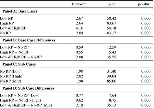
of the CIG range. Table 8 reports share turnover, defined as the ratio
of volume to shares outstanding in percent, on the day of the event. In
panel A, when analysts forecast at the low (high) point of the CIG range,
share turnover is 2.67% (2.64%). When analysts forecast at the low and
high points of the CIG range, share turnover is much higher at 4.16%.
Finally, when analysts forecast away from the points of the CIG range,
share turnover is lower than the other three categories at 2.09%. In panel
B, I use the No RP category as a benchmark to determine whether the
differences are statistically significant. The Low RP category has 0.59 percentage points more turnover than the No RP category, while the High
RP category has 0.55 percentage points more turnover than the No RP
category. The Low & High RP share turnover is substantially higher that
the No RP category, with a difference of 2.08 percentage points. These differences are statistically significant at the 1% level. To put these num-bers in perspective, the Low (High) RP category has 28% (26%) more
share turnover than the No RP category, while the Low & High RP has
100% more share turnover than the No RP category. Panel C reports
the results of the No RP sub categories, split into Low, High, and Mid.
The No RP (Low) sub category has share turnover of 1.9%, while the
No RP (High) sub category has share turnover of 2.02%, and the No RP
(Mid) sub category has share turnover of 1.98%. Panel D reports the
differences between the Low, High and Low & High RP categories, and the No RP sub categories. Relative to the No RP subcategories, the Low
and High RP share turnover are qualitatively similar to those in panel B,
with Low RP – No RP (Low) yielding a share turnover difference of 0.77 percentage points and High RP – No RP (High) yielding a share turnover
difference of 0.62 percentage points. The Low & High RP share turnover is again substantially higher that the No RP (Mid) category, with a di ffer-ence of 2.19 percentage points. These differences represent 41%, 31% and 111% more share turnover than the respective benchmarks.
Table 9 verifies the robustness of the share turnover results in table 8
in a multivariate regression framework. Along with the control variables
included in table 5 and table 7 regressions, I also include the natural
logarithm of the firm’s market capitalization in millions of dollars to
capture size, the ratio of book equity to market capitalization to capture
growth/value, and the firm’s stock market return in the year prior to the event to capture momentum. Model 1 looks at the control variables in
isolation, while model 2 includes Low RP, High RP and Low & High
CIG range endpoints as references. The results are consistent with the
univariate results in table 8. The coefficient on Low RP, High RP, and Low & High RP are all significantly positive at the 1% level, indicating
that share turnover is reliably higher when analysts forecast at the low,
high, an low & high points of the CIG range, respectively. Economically,
forecasting at the low point of the CIG range leads to a 0.53 percentage
point increase in share turnover during the event, while forecasting at the
high point of the CIG range leads to a 0.4 percentage point increase, and
forecasting at both the low & high points of the CIG range leads to a 1.83
percentage point increase. The economic significance is qualitatively
similar to that in panel B of table 8.
The results in this section show that investors overreact to analyst
reference points. Indeed, investors bid down (up) the prices of stocks for
which analysts have provided a forecast exactly equal to the low (high)
endpoint of the CIG range more so than for other comparable forecasts.
Moreover, the stock prices of firms for which analysts have provided a
forecast exactly equal to the low (high) point of the CIG range correct
upward (downward) in the subsequent month, suggesting that investors’
reaction was too pronounced to begin with. Furthermore, investors tend
to make too many trades when they are faced with analyst reference
points, suggesting that they may be overconfident in situations where
5
Conclusions
This paper contributes to the discussion on analysts’ role in
disseminat-ing information to the public. All of the evidence supports the notion
that analysts use the company guidance range as a reference. It may
seem obvious that analysts use the company issued guidance in order
to make their forecasts. However, the material point is that there is a
sharp change in analysts’ forecasting behavior around the endpoints of
the company issued guidance. Inexperienced or unskilled analysts tend
to be the ones who forecast outside of the guidance range, and this is
to the detriment of their reputation given the lower accuracy associated
with these forecasts. There are various incentives which may induce
analysts to engage in this type of forecasting behavior. Inexperienced
analysts have no reputation to speak of, and therefore have no
disin-centive to be bold with their forecasts. Furthermore, if inexperienced
analysts are trying to distinguish themselves from other analysts in order
to increase the likelihood of having a long career, they may have a direct
incentive to provide bold forecasts. Another possibility is that some
an-alysts may have performed poorly in the past, which negatively affects their reputation. In order to reestablish this reputation, they may find
it worthwhile to issue bold forecasts. Lastly, some analysts may lack
the skill to be good forecasters or may not understand the informational
content in company issued guidance.
be-havior, the fact that they use the company issued guidance endpoints as
a frame of reference may have an impact on stock markets. For
exam-ple, an analyst may have valuable private information about a firm. This
private information could lead this analyst to make a forecast outside of
the guidance range. However, given the various incentives mentioned
above, it may be more beneficial for this analyst to make a forecast on
one of the endpoints of the guidance range. Market participants, who
may or may not realize this, are left with less information than if the
analyst’s true beliefs had been revealed. As such, this paper also adds
to the discussion on market efficiency. Through its impact on investors, analyst reference points are associated with stock market overreaction
followed by a correction. Moreover, this overreaction is accompanied
by excessive trading. Together, these results suggests that in situations
of information uncertainty, investor overconfidence can lead to
References
Baker, M., X. Pan, and J. Wurgler, 2012, The effect of reference point prices on mergers and acquisitions, Journal of Financial Economics
106, 49–71.
Barberis, N., A. Shleifer, and R. Vishny, 1998, A model of investor
sen-timent, Journal of Financial Economics 49, 307–343.
Campbell, S.D., and S.A. Sharpe, 2009, Anchoring bias in consensus
forecasts and its effect on market prices, Journal of Financial and Quantitative Analysis44, 369–390.
Carhart, M.M., 1997, On persistence in mutual fund performance,
Jour-nal of Finance52, 57–82.
Cen, L., G. Hilary, and J. Wei, 2013, The role of anchoring bias in the
equity market: Evidence from analysts’ earnings forecasts and stock
returns, Journal of Financial and Quantitative Analysis 48, 47–76.
Chopra, N., J. Lakonishok, and J.R. Ritter, 1992, Measuring abnormal
performance, Journal of Financial Economics 31, 235–268.
Clement, M.B., and S.Y. Tse, 2005, Financial analyst characteristics and
herding behavior in forecasting, Journal of Finance 60, 307–341.
Cutler, D.M., J.M. Poterba, and L.H. Summers, 1991, Speculative
Daniel, K., D. Hirshleifer, and A. Subrahmanyam, 1998, Investor
psy-chology and security market under- and overreactions, Journal of
Fi-nance53, 1839–1885.
De Bondt, W., and R. Thaler, 1985, Does the stock market overreact?,
Journal of Finance40, 793–805.
, 1987, Further evidence on investor overreaction and stock
mar-ket seasonality, Journal of Finance 42, 557–581.
Dougal, C., J. Engelberg, C.A. Parsons, and E.D. Van Wesep, 2012,
An-choring and the cost of capital, Working Paper pp. 1–46.
Fama, E.F., and K.R. French, 1988, Permanent and temporary
compo-nents of stock prices, Journal of Political Economy 96, 246–273.
, 1993, Common risk factors in the returns on stocks and bonds,
Journal of Financial Economics33, 3–56.
Hong, H., and J.C. Stein, 1999, A unified theory of underreaction,
mo-mentum trading, and overreaction in asset markets, Journal of Finance
54, 2143–2184.
Kahneman, D., 1992, Reference points, anchors, norms, and mixed
feel-ings, Organizational Behavior and Human Decision Processes 51,
296–312.
, and A. Tversky, 1979, Prospect theory: An analysis of decision
Ko, J.K., and Z. Huang, 2007, Arrogance can be a virtue:
Overconfi-dence, information acquisition, and market efficiency, Journal of Fi-nancial Economics84, 529–560.
La Porta, R., 1996, Expectations and the cross-section of stock returns,
Journal of Finance51, 1715–1742.
, J. Lakonishok, A. Shleifer, and R.W. Vishny, 1997, Good news
for value stocks: Further evidence on market efficiency, Journal of Finance52, 859–874.
Lakonishok, J., A. Shleifer, and R.W. Vishny, 1994, Contrarian
invest-ment, extrapolation, and risk, Journal of Finance 49, 1541–1578.
Ljungqvist, A., and W.J. Wilhelm Jr., 2005, Does prospect theory explain
ipo market behavior?, Journal of Finance 60, 1759–1790.
Loughran, T., and J.R. Ritter, 2002, Why don’t issuers get upset about
leaving money on the table in ipos?, Review of Financial Studies 15,
413–443.
Odean, T., 1998, Volume, volatility, price, and profit when all traders are
above average, Journal of Finance 53, 1887–1934.
, 1999, Do investors trade too much?, American Economic
Re-view89, 1279–1298.
Poterba, J.M., and L.H. Summers, 1988, Mean reversion in stock prices,
Statman, M., S. Thorley, and K. Vorkink, 2006, Investor overconfidence
and trading volume, Review of Financial Studies 19, 1531–1565.
Tversky, A., and D. Kahneman, 1974, Judgment under uncertainty:
2001 2002 2003 2004 2005 2006 2007 2008 2009 2010 2011 Year 0 5000 10000 15000 20000 25000 F re qu en cy 0 20 40 60 80 100 P er ce nt
Analyst Forecast > CIG High Analyst Forecast = CIG High
CIG Low < Analyst Forecast < CIG High Analyst Forecast = CIG Low
Analyst Forecast < CIG Low Cumulative Frequency
Figure 1: Yearly Frequencies of Analyst Forecasts Relative to Company Issued Guidance Endpoints
This figure reports the yearly frequency and percentage of analyst forecasts relative to the company issued guidance endpoints. Analyst Forecast is the analyst quarterly EPS forecast. CIG Low is the low point of the company issued quarterly EPS guidance range. CIG High is the high point of the company issued quarterly EPS guidance range.
-10 -9 -8 -7 -6 -5 -4 -3 -2 -1 0 1 2 3 4 5 6 7 8 9 10 Event-Time (days) -0.75 -0.50 -0.25 0.00 0.25 0.50 A bn or m al R et ur n (% ) No RP Low & High RP
High RP Low RP
(a) Base Cases
-10 -9 -8 -7 -6 -5 -4 -3 -2 -1 0 1 2 3 4 5 6 7 8 9 10 Event-Time (days) -0.75 -0.50 -0.25 0.00 0.25 0.50 A bn or m al R et ur n (% ) No RP (High) High RP No RP (Low) Low RP
(b) Base and Sub Cases
Figure 2: Event-Window Average Abnormal Returns
This figure reports the mean abnormal return for each day of the [-10,+10] event window for various sub-samples. Low RP equals 1 when at least one analyst quarterly EPS forecast equals the low point of the company issued quarterly EPS guidance range on the day of the event, and 0 otherwise. High RP equals 1 when at least one analyst quarterly EPS forecast equals the high point of the company issued quarterly EPS guidance range on the day of the event, and 0 otherwise. Low & High RP equals 1 when at least one analyst quarterly EPS forecast equals the low point and at least one analyst quarterly EPS forecast equals the high point of the company issued quarterly EPS guidance range on the day of the event, and 0 otherwise. No RP equals 1 when no analyst quarterly EPS forecast equals the low or high point of the company issued quar-terly EPS guidance range on the day of the event, and 0 otherwise. No RP (Low) equals 1 when all analyst quarterly EPS forecasts are less than the low point of the company issued quarterly EPS guidance range on the day of the event, and 0 otherwise. No RP (High) equals 1 when all analyst quarterly EPS forecasts are greater than the high point of the company issued quarterly EPS guidance range on the day of the event, and 0 otherwise. The abnormal return is calculated using a Fama-French-Carhart 4-factor model to estimate the expected return.
-10 -8 -6 -4 -2 0 2 4 6 8 10 12 14 16 18 20 22 24 26 28 30 Event-Time (days) -2.0 -1.5 -1.0 -0.5 0.0 0.5 1.0 C um ul at iv e A bn or m al R et ur n (% ) No RP Low & High RP
High RP Low RP
(a) Base Cases
-10 -8 -6 -4 -2 0 2 4 6 8 10 12 14 16 18 20 22 24 26 28 30 Event-Time (days) -2.0 -1.5 -1.0 -0.5 0.0 0.5 1.0 C um ul at iv e A bn or m al R et ur n (% ) No RP (High) High RP No RP (Low) Low RP
(b) Base and Sub Cases
Figure 3: Event-Window Average Cumulative Abnormal Returns
This figure reports the mean cumulative abnormal return over the [-10,+30] event window for various sub-samples. Low RP equals 1 when at least one analyst quarterly EPS forecast equals the low point of the company issued quarterly EPS guidance range on the day of the event, and 0 otherwise. High RP equals 1 when at least one analyst quarterly EPS forecast equals the high point of the company issued quarterly EPS guidance range on the day of the event, and 0 otherwise. Low & High RP equals 1 when at least one analyst quarterly EPS forecast equals the low point and at least one analyst quarterly EPS forecast equals the high point of the company issued quarterly EPS guidance range on the day of the event, and 0 otherwise. No RP equals 1 when no analyst quarterly EPS forecast equals the low or high point of the company issued quar-terly EPS guidance range on the day of the event, and 0 otherwise. No RP (Low) equals 1 when all analyst quarterly EPS forecasts are less than the low point of the company issued quarterly EPS guidance range on the day of the event, and 0 otherwise. No RP (High) equals 1 when all analyst quarterly EPS forecasts are greater than the high point of the company issued quarterly EPS guidance range on the day of the event, and 0 otherwise.
Table 1: Analyst Forecast Frequency and Performance Relative to Company Is-sued Guidance Endpoints
This table reports the frequency and percentage of analyst forecasts relative to the comapny issued guidance endpoints, as well as analyst ex post performance. Analyst Forecast is the analyst quarterly EPS forecast. CIG Low is the low point of the company issued quarterly EPS guidance range. CIG High is the high point of the company issued quarterly EPS guidance range. Error is the percentage difference between the an-alyst quarterly EPS forecast and realized quarterly EPS. Accuracy is the absolute value of the percentage difference between the analyst quarterly EPS forecast and realized quarterly EPS.
Subsample Frequency Percent Error (%) Accuracy (%) Analyst Forecast< CIG Low 8,861 6.13 −19.02 52.54 Analyst Forecast= CIG Low 17,338 11.99 −2.31 28.52 CIG Low< Analyst Forecast < CIG High 69,838 48.31 −0.50 26.61 Analyst Forecast= CIG High 31,890 22.06 −0.47 20.76 Analyst Forecast> CIG High 16,639 11.51 3.97 30.92
Table 2: Analyst Performance Multivariate Regressions
This table reports the coefficients from a regression of analyst forecast errors and analyst forecast accuracy on multiple variables. Analyst Forecast is the analyst quarterly EPS forecast. CIG Low is the low point of the company issued quarterly EPS guidance range. CIG High is the high point of the company issued quarterly EPS guidance range. CIG Range Midpoint is the middle point of the company issued quarterly EPS guidance range. Market Cap is the number of shares outstanding multiplied by the price, in millions of dollars. Book-to-Market is the book value of common equity divided by the market capitalization. Momentum is the firm’s monthly compounded stock return over the past year. Analyst Coverage is the number of analysts that have provided an EPS forecast for the firm over the past year. Standardized Unexpected EPS is the ratio of the quarterly earnings surprise to the standard deviation of earnings surprises over the past four quarters. EPS Volatility is the standard deviation of realized quarterly EPS over the past four quarters. Error is the percentage difference between the analyst quarterly EPS forecast and realized quarterly EPS. Accuracy is the absolute value of the percentage difference between the analyst quarterly EPS forecast and realized quarterly EPS. The numbers in parentheses are t-statistics based on simple t-tests. ***, ** or * signify that the test statistic is significant at the 1, 5 or 10% two-tailed level, respectively.
Error (%) Accuracy (%) Model 1 Model 2 Model 1 Model 2 Analyst Forecast< CIG Low −14.22∗∗∗ 18.48∗∗∗
(−12.53) (17.26) Analyst Forecast= CIG Low −0.73 −0.62
(−0.88) (−0.80) Analyst Forecast= CIG High 0.95 −4.54∗∗∗
(1.45) (−7.37) Analyst Forecast> CIG High 3.41∗∗∗ 4.58∗∗∗
(4.05) (5.79)
Analyst Forecast 45.39∗∗∗ 36.65∗∗∗ −40.85∗∗∗ −33.06∗∗∗ (22.02) (16.96) (−20.98) (−16.23) CIG Range Midpoint −31.18∗∗∗ −22.86∗∗∗ 10.85∗∗∗ 3.39∗ (−15.72) (−11.01) (5.80) (1.73) Ln(Market Cap) −0.63∗∗∗ −0.54∗∗ −2.64∗∗∗ −2.76∗∗∗ (−2.69) (−2.31) (−12.01) (−12.61) Book-to-Market 0.30 0.55 10.17∗∗∗ 9.52∗∗∗ (0.38) (0.70) (13.78) (12.87) Momentum −2.29∗∗∗ −2.47∗∗∗ −2.51∗∗∗ −2.20∗∗∗ (−4.51) (−4.86) (−5.23) (−4.59) Analyst Coverage −0.09∗∗∗ −0.11∗∗∗ −0.19∗∗∗ −0.17∗∗∗ (−2.67) (−3.10) (−5.75) (−5.15) Standardized Unexpected EPS −0.54∗∗∗ −0.55∗∗∗ −0.10∗∗∗ −0.10∗∗∗
(−19.69) (−19.90) (−3.98) (−4.02) EPS Volatility −2.74∗ −2.59∗ 45.48∗∗∗ 43.77∗∗∗ (−1.88) (−1.77) (33.04) (31.73) Intercept 5.18∗ 4.55 70.61∗∗∗ 71.96∗∗∗ (1.66) (1.45) (23.96) (24.33) Adj. R2(%) 0.8 0.9 3.8 4.1 N 136,445 136,445 136,445 136,445
T able 3: Analyst F or ecasting Decision Multi v ariate Logistic Regr essions This table reports the coe ffi cients from logistic re gressions of the decision to forecast within a specific cate gory on analyst charcteristics and control v ariables. Analyst F orecast is the analyst quarterly EPS forecast. CIG Lo w is the lo w point of the compan y issued quarterly EPS guidance range. CIG High is the high point of the compan y issued quarterly EPS guidance range. Experience is the number of years between the analyst’ s first forecast and current forecast. P ast Error is the analyst’ s av erage Error o v er the past year . P ast Accurac y is the analyst’ s av erage Accurac y o v er the past year . Error is the di ff erence between the analyst quarterly EPS forecast and realized quarterly EPS, scaled by the absolute v alue of realized quarterly EPS. Accurac y is the absolute v alue of the di ff erence between the analyst quarterly EPS forecast and realized quarterly EPS, scaled by the absolute v alue of realized quarterly EPS. CIG Range Midpoint is the middle point of the compan y issued quarterly EPS guidance range. Mark et Cap is the number of shares outstanding multiplied by the price, in millions of dollars. Book-to-Mark et is the book v alue of common equity di vided by the mark et capitalization. Momentum is the firm’ s monthly compounded stock return o v er the past year . Analyst Co v erage is the number of analysts that ha v e pro vided an EPS forecast for the firm o v er the past year . Standardized Une xpected EPS is the ratio of the quarterly earnings surprise to the standard de viation of earnings surprises o v er the past four quarters. EPS V olatility is the standard de viation of realized quarterly EPS o v er the past four quarters. The numbers in parentheses are W ald Chi Square statistics. ***, ** or * signify that the test statistic is significant at the 1, 5 or 10% tw o-tailed le v el, respecti v ely . Analyst F orecast Analyst F orecast CIG Lo w Analyst F orecast Analyst F orecast < = < Analyst F orecast < = > CIG Lo w CIG Lo w CIG High CIG High CIG High Experience − 0 .021 ∗ ∗ ∗ 0 .003 ∗ ∗ 0 .004 ∗ ∗ ∗ 0 .003 ∗ ∗ − 0 .007 ∗ ∗ ∗ (85 .62) (4 .34) (17 .65) (5 .46) (16 .30) P ast Error − 0 .248 ∗ ∗ ∗ 0 .215 ∗ ∗ ∗ − 0 .009 0 .061 ∗ ∗ 0 .013 (99 .22) (42 .71) (0 .27) (5 .50) (0 .30) P ast Accurac y 0 .451 ∗ ∗ ∗ − 0 .236 ∗ ∗ ∗ 0 .016 − 0 .294 ∗ ∗ ∗ 0 .049 ∗ ∗ (333 .85) (54 .26) (0 .97) (137 .39) (4 .35) CIG Range Midpoint 0 .420 ∗ ∗ ∗ − 0 .271 ∗ ∗ ∗ 0 .387 ∗ ∗ ∗ − 0 .345 ∗ ∗ ∗ − 0 .288 ∗ ∗ ∗ (185 .42) (101 .98) (534 .36) (251 .83) (154 .65) Ln(Mark et Cap) 0 .001 − 0 .062 ∗ ∗ ∗ 0 .012 ∗ ∗ − 0 .008 0 .048 ∗ ∗ ∗ (0 .01) (61 .82) (5 .21) (1 .57) (37 .77) Book-to-Mark et 0 .238 ∗ ∗ ∗ − 0 .187 ∗ ∗ ∗ 0 .348 ∗ ∗ ∗ − 0 .634 ∗ ∗ ∗ 0 .013 (53 .71) (46 .60) (349 .88) (578 .36) (0 .23) Momentum − 0 .295 ∗ ∗ ∗ − 0 .326 ∗ ∗ ∗ − 0 .126 ∗ ∗ ∗ 0 .295 ∗ ∗ ∗ 0 .117 ∗ ∗ ∗ (109 .71) (250 .97) (118 .70) (510 .23) (56 .15) Analyst Co v erage − 0 .009 ∗ ∗ ∗ 0 .003 ∗ ∗ ∗ − 0 .009 ∗ ∗ ∗ 0 .010 ∗ ∗ ∗ 0 .005 ∗ ∗ ∗ (31 .64) (7 .11) (119 .96) (115 .30) (14 .50) Standardized Une xpected EPS − 0 .003 ∗ ∗ ∗ − 0 .008 ∗ ∗ ∗ − 0 .002 ∗ ∗ 0 .020 ∗ ∗ ∗ 0 .014 ∗ ∗ ∗ (11 .97) (137 .21) (6 .58) (170 .29) (66 .76) EPS V olatility 0 .046 − 0 .914 ∗ ∗ ∗ − 0 .072 ∗ ∗ − 0 .691 ∗ ∗ ∗ 1 .112 ∗ ∗ ∗ (0 .54) (208 .31) (5 .05) (211 .23) (733 .43) Intercept − 2 .922 ∗ ∗ ∗ − 0 .736 ∗ ∗ ∗ − 0 .401 ∗ ∗ ∗ − 0 .817 ∗ ∗ ∗ − 2 .903 ∗ ∗ ∗ (413 .27) (47 .94) (33 .83) (93 .55) (758 .70) AIC 59406.18 96524.81 184867.8 139093.7 94914.50 SC 59514.08 96632.70 184975.7 139201.6 95022.39 -2 Log L 59384.18 96502.81 184845.8 139071.7 94892.50 N 134,427 134,427 134,427 134,427 134,427
T able 4: Ev ent-Day Abnormal Retur ns This table reports the mean 1-day abnormal returns and standardized abnormal returns, as well as mean di ff erences with benchmark portfolios on v arious subsamples. Lo w RP equals 1 when at least one analyst quarterly EPS forecast equals the lo w point of the compan y issued quarterly EPS guidance range on the day of the ev ent, and 0 otherwise. High RP equals 1 when at least one analyst quarterly EPS forecast equals the high point of the compan y issued quarterly EPS guidance range on the day of the ev ent, and 0 otherwise. Lo w & High RP equals 1 when at least one analyst quarterly EPS forecast equals the lo w point and at least one analyst quarterly EPS forecast equals the high point of the compan y issued quarterly EPS guidance range on the day of the ev ent, and 0 otherwise. No RP equals 1 when no analyst quarterly EPS forecast equals the lo w or high point of the compan y issued quarterly EPS guidance range on the day of the ev ent, and 0 otherwise. No RP (Lo w) equals 1 when all analyst quarterly EPS forecasts are less than the lo w point of the compan y issued quarterly EPS guidance range on the day of the ev ent, and 0 otherwise. No RP (Mid) equals 1 when all analyst quarterly EPS forecasts are more than the lo w point and less than the high point of the compan y issued quarterly EPS guidance range on the day of the ev ent, and 0 otherwise. No RP (High) equals 1 when all analyst quarterly EPS forecasts are greater than the high point of the compan y issued quarterly EPS guidance range on the day of the ev ent, and 0 otherwise. AR is the abnormal return during the ev ent day , using a F ama-French-Carhart 4-f actor model to estimate the expected return. SAR is the standardized abnormal return during the ev ent day , using a F ama-French-Carhart 4-f actor model to estimate the expected return. AR (%) SAR (%) Return t-stat p-v alue Return t-stat p-v alue P anel A: Base Cases Lo w RP − 0 .59 − 6 .90 0 .000 − 25 .84 − 7 .36 0 .000 High RP 0 .10 1 .90 0 .057 7 .81 3 .48 0 .000 Lo w & High RP − 0 .22 − 1 .74 0 .082 − 8 .33 − 1 .58 0 .114 No RP − 0 .06 − 1 .63 0 .104 − 0 .92 − 0 .62 0 .538 P anel B: Base Case Di ff er ences Lo w RP − No RP − 0 .53 − 6 .68 0 .000 − 24 .92 − 7 .52 0 .000 High RP − No RP 0 .16 2 .57 0 .010 8 .73 3 .36 0 .001 Lo w & High RP − No RP − 0 .16 − 1 .62 0 .105 − 7 .41 − 1 .81 0 .070 P anel C: Sub Cases No RP (Lo w) − 0 .19 − 1 .99 0 .046 − 6 .77 − 1 .58 0 .114 No RP (High) − 0 .37 − 3 .63 0 .000 − 6 .50 − 1 .88 0 .061 No RP (Mid) − 0 .01 − 0 .14 0 .885 − 0 .23 − 0 .12 0 .903 P anel D: Sub Case Di ff er ences Lo w RP − No RP (Lo w) − 0 .40 − 2 .45 0 .014 − 19 .07 − 2 .83 0 .005 High RP − No RP (High) 0 .47 3 .89 0 .000 14 .30 2 .85 0 .004 Lo w & High RP − No RP (Mid) − 0 .21 − 2 .01 0 .044 − 8 .10 − 1 .83 0 .068
Table 5: Event-Day Abnormal Return Multivariate Regressions
This table reports the coefficients from a regression of 1-day cumulative abnormal returns and standardized cululative abnormal returns on multiple variables. Low RP equals 1 when at least one analyst quarterly EPS forecast equals the low point of the company issued quarterly EPS guidance range on the day of the event, and 0 otherwise. High RP equals 1 when at least one analyst quarterly EPS forecast equals the high point of the company issued quarterly EPS guidance range on the day of the event, and 0 otherwise. Low & High RP equals 1 when at least one analyst quarterly EPS forecast equals the low point and at least one analyst quarterly EPS forecast equals the high point of the company issued quarterly EPS guidance range on the day of the event, and 0 otherwise. Mean Analyst Forecast is the average analyst quarterly EPS forecast on the event day. CIG Range Midpoint is the middle point of the company issued quarterly EPS guidance range. Analyst Coverage is the number of analysts that have provided an EPS forecast for the firm over the past year. Standardized Unexpected EPS is the ratio of the quarterly earnings surprise to the standard deviation of earnings surprises over the past four quarters. EPS Volatility is the standard deviation of realized quarterly EPS over the past four quarters. AR is the abnormal return during the event day, using a Fama-French-Carhart 4-factor model to estimate the expected return. SAR is the standardized abnormal return during the event day, using a Fama-French-Carhart 4-factor model to estimate the expected return. The numbers in parentheses are t-statistics based on simple t-tests. ***, ** or * signify that the test statistic is significant at the 1, 5 or 10% two-tailed level, respectively.
AR (%) SAR (%)
Model 1 Model 2 Model 1 Model 2
Low RP −0.41∗∗∗ −20.55∗∗∗
(−4.78) (−5.56)
High RP 0.14∗∗ 8.10∗∗∗
(2.07) (2.76)
Low & High RP −0.16 −7.31∗
(−1.51) (−1.66) Mean Analyst Forecast 0.59∗∗∗ 0.51∗∗ 19.45∗∗ 15.06
(2.62) (2.25) (2.02) (1.56) CIG Range Midpoint 0.11 0.18 4.96 8.19
(0.53) (0.80) (0.53) (0.88) Analyst Coverage 0.00 0.00 −0.03 −0.02
(0.27) (0.32) (−0.18) (−0.15) Standardized Unexpected EPS 0.05∗∗∗ 0.05∗∗∗ 2.38∗∗∗ 2.33∗∗∗
(16.36) (16.04) (17.23) (16.85) EPS Volatility 0.35∗∗ 0.33∗∗ 19.07∗∗∗ 18.29∗∗∗ (2.25) (2.13) (2.87) (2.74) Intercept −0.54∗∗∗ −0.50∗∗∗ −19.09∗∗∗ −17.11∗∗∗ (−8.44) (−7.08) (−6.98) (−5.73) Adj. R2(%) 0.9 1.0 0.9 1.0 N 42,737 42,737 42,737 42,737
T able 6: Short-Run Cumulati v e Abnormal Retur ns This table reports the mean 30-day cumulati v e abnormal returns and standardized cumulati v e abnormal returns, as well as mean di ff erences with benchmark portfolios on v arious subsamples. Lo w RP equals 1 when at least one analyst quarterly EPS forecast equals the lo w point of the compan y issued quarterly EPS guidance range on the day of the ev ent, and 0 otherwise. High RP equals 1 when at least one analyst quarterly EPS forecast equals the high point of the compan y issued quarterly EPS guidance range on the day of the ev ent, and 0 otherwise. Lo w & High RP equals 1 when at least one analyst quarterly EPS forecast equals the lo w point and at least one analyst quarterly EPS forecast equals the high point of the compan y issued quarterly EPS guidance range on the day of the ev ent, and 0 otherwise. No RP equals 1 when no analyst quarterly EPS forecast equals the lo w or high point of the compan y issued quarterly EPS guidance range on the day of the ev ent, and 0 otherwise. No RP (Lo w) equals 1 when all analyst quarterly EPS forecasts are less than the lo w point of the compan y issued quarterly EPS guidance range on the day of the ev ent, and 0 otherwise. No RP (Mid) equals 1 when all analyst quarterly EPS forecasts are more than the lo w point and less than the high point of the compan y issued quarterly EPS guidance range on the day of the ev ent, and 0 otherwise. No RP (High) equals 1 when all analyst quarterly EPS forecasts are greater than the high point of the compan y issued quarterly EPS guidance range on the day of the ev ent, and 0 otherwise. CAR is the cumulati v e abnormal return during the [+ 1, + 30] ev ent windo w , using a F ama-French-Carhart 4-f actor model to estimate the expected return. SCAR is the standardized cumulati v e abnormal return during the [+ 1, + 30] ev ent windo w , using a F ama-French-Carhart 4-f actor model to estimate the expected return. CAR (%) SCAR (%) Return t-stat p-v alue Return t-stat p-v alue P anel A: Base Cases Lo w RP 0 .70 21 .35 0 .000 5 .13 22 .01 0 .000 High RP − 0 .93 − 45 .23 0 .000 − 7 .65 − 49 .80 0 .000 Lo w & High RP − 0 .13 − 3 .48 0 .000 − 1 .35 − 4 .99 0 .000 No RP − 0 .06 − 3 .24 0 .001 − 0 .57 − 4 .40 0 .000 P anel B: Base Case Di ff er ences Lo w RP − No RP 0 .76 20 .85 0 .000 5 .70 21 .51 0 .000 High RP − No RP − 0 .87 − 31 .53 0 .000 − 7 .08 − 34 .62 0 .000 Lo w & High RP − No RP − 0 .07 − 1 .64 0 .101 − 0 .78 − 2 .50 0 .012 P anel C: Sub Cases No RP (Lo w) 0 .29 5 .23 0 .000 3 .51 7 .94 0 .000 No RP (High) − 0 .21 − 3 .45 0 .001 − 4 .25 − 12 .16 0 .000 No RP (Mid) − 0 .01 − 0 .49 0 .623 − 0 .08 − 0 .51 0 .613 P anel D: Sub Case Di ff er ences Lo w RP − No RP Lo w 0 .42 6 .27 0 .000 1 .62 3 .33 0 .001 High RP − No RP High − 0 .72 − 13 .90 0 .000 − 3 .39 − 9 .31 0 .000 Lo w & High RP − No RP Mid − 0 .12 − 2 .75 0 .006 − 1 .27 − 3 .97 0 .000
Table 7: Short-Run Cumulative Abnormal Return Multivariate Regressions
This table reports the coefficients from a regression of 30-day cumulative abnormal returns and standardized cululative abnormal returns on multiple variables. Low RP equals 1 when at least one analyst quarterly EPS forecast equals the low point of the company issued quarterly EPS guidance range on the day of the event, and 0 otherwise. High RP equals 1 when at least one analyst quarterly EPS forecast equals the high point of the company issued quarterly EPS guidance range on the day of the event, and 0 otherwise. Low & High RP equals 1 when at least one analyst quarterly EPS forecast equals the low point and at least one analyst quarterly EPS forecast equals the high point of the company issued quarterly EPS guidance range on the day of the event, and 0 otherwise. Mean Analyst Forecast is the average analyst quarterly EPS forecast on the event day. CIG Range Midpoint is the middle point of the company issued quarterly EPS guidance range. Analyst Coverage is the number of analysts that have provided an EPS forecast for the firm over the past year. Standardized Unexpected EPS is the ratio of the quarterly earnings surprise to the standard deviation of earnings surprises over the past four quarters. EPS Volatility is the standard deviation of realized quarterly EPS over the past four quarters. CAR is the cumulative abnormal return during the [+1,+30] event window, using a Fama-French-Carhart 4-factor model to estimate the expected return. SCAR is the standardized cumulative abnormal return during the [+1,+30] event window, using a Fama-French-Carhart 4-factor model to estimate the expected return. The numbers in parentheses are t-statistics based on simple t-tests. ***, ** or * signify that the test statistic is significant at the 1, 5 or 10% two-tailed level, respectively.
CAR (%) SCAR (%) Model 1 Model 2 Model 1 Model 2
Low RP 0.67∗∗∗ 5.25∗∗∗
(3.38) (3.57)
High RP −0.94∗∗∗ −7.05∗∗∗
(−5.99) (−6.03)
Low & High RP −0.37 −1.83
(−1.56) (−1.04) Mean Analyst Forecast −2.46∗∗∗ −2.15∗∗∗ −20.54∗∗∗ −18.22∗∗∗
(−4.80) (−4.20) (−5.38) (−4.76) CIG Range Midpoint 1.16∗∗ 0.89∗ 10.73∗∗∗ 8.72∗∗
(2.34) (1.80) (2.90) (2.35) Analyst Coverage 0.04∗∗∗ 0.04∗∗∗ 0.13∗∗ 0.16∗∗∗
(4.33) (4.90) (2.06) (2.58) Standardized Unexpected EPS −0.02∗∗∗ −0.02∗∗ −0.11∗∗ −0.09∗ (−2.69) (−2.32) (−2.04) (−1.65) EPS Volatility −0.38 −0.45 −0.82 −1.25 (−1.08) (−1.27) (−0.31) (−0.47) Intercept −0.11 0.02 0.31 1.20 (−0.78) (0.10) (0.29) (1.01) Adj. R2(%) N 42,737 42,737 42,737 42,737
Table 8: Event-Day Share Turnover
This table reports the mean share turnover, as well as mean differences with benchmark portfolios on various subsamples. Low RP equals 1 when at least one analyst quarterly EPS forecast equals the low point of the company issued quarterly EPS guidance range on the day of the event, and 0 otherwise. High RP equals 1 when at least one analyst quarterly EPS forecast equals the high point of the company issued quarterly EPS guidance range on the day of the event, and 0 otherwise. Low & High RP equals 1 when at least one analyst quarterly EPS forecast equals the low point and at least one analyst quarterly EPS forecast equals the high point of the company issued quarterly EPS guidance range on the day of the event, and 0 otherwise. No RP equals 1 when no analyst quarterly EPS forecast equals the low or high point of the company issued quarterly EPS guidance range on the day of the event, and 0 otherwise. No RP (Low) equals 1 when all analyst quarterly EPS forecasts are less than the low point of the company issued quarterly EPS guidance range on the day of the event, and 0 otherwise. No RP (Mid) equals 1 when all analyst quarterly EPS forecasts are more than the low point and less than the high point of the company issued quarterly EPS guidance range on the day of the event, and 0 otherwise. No RP (High) equals 1 when all analyst quarterly EPS forecasts are greater than the high point of the company issued quarterly EPS guidance range on the day of the event, and 0 otherwise. Turnover is the ratio of volume to shares outstanding in percent on the day of the event.
Turnover t-stat p-value Panel A: Base Cases
Low RP 2.67 50.42 0.000
High RP 2.64 83.67 0.000
Low & High RP 4.16 50.18 0.000
No RP 2.09 103.17 0.000
Panel B: Base Case Differences
Low RP − No RP 0.59 12.59 0.000
High RP − No RP 0.55 15.43 0.000
Low & High RP − No RP 2.08 35.55 0.000 Panel C: Sub Cases
No RP (Low) 1.90 31.40 0.000
No RP (High) 2.02 39.04 0.000
No RP (Mid) 1.98 85.06 0.000
Panel D: Sub Case Differences
Low RP − No RP (Low) 0.77 7.64 0.000 High RP − No RP (High) 0.62 8.75 0.000 Low & High RP − No RP (Mid) 2.19 35.13 0.000