Centre de Recherche en économie de l’Environnement, de l’Agroalimentaire, des Transports et de l’Énergie
Center for Research on the economics of the Environment, Agri-food, Transports and Energy
_______________________
Bernard: Department of Economics, University of Ottawa; GREEN and CREATE, Université Laval. Mailing address: 55 Laurier Avenue East, Desmarais Building room 3184, Ottawa, Ont. Canada K1N 6N5. Tel.: 613 562 5800-1374; [email protected]
Gavin: University of Toronto
Khalaf: Economics Department and CMFE, Carleton University; CIREQ, Université de Montréal; GREEN and CREATE, Université Laval. Mailing address: Economics Department, Carleton University, Loeb Building 1125 Colonel By Drive, Ottawa, Ont. Canada K1S 5B6. Tel.: 613 520 2600-8697; [email protected]
Voia: Economics Department and CMFE, Carleton University. Mailing address : same address as Khalaf. Tel.: 613 520 2600-3546;
This work supported by the Canadian Network of Centres of Excellence [program on Mathematics of Information Technology and Complex Systems (MITACS)], the Social Sciences and Humanities Research Council of Canada, and the Fonds de recherche sur la société et la culture, Québec. We thank Trudy Ann Cameron, John Livernois and Carlos Ordás-Criado for useful comments and suggestions.
Les cahiers de recherche du CREATE ne font pas l’objet d’un processus d’évaluation par les pairs/CREATE working papers do not undergo a peer review process.
The Environmental Kuznets Curve: Tipping Points,
Uncertainty and Weak Identification
Jean-Thomas Bernard
Michael Gavin
Lynda Khalaf
Marcel Voia
Cahier de recherche/Working Paper 2011-4
Abstract:
We consider an empirical estimation of the Environmental Kuznets Curve (EKC) for carbon
dioxide and sulphur, with a focus on confidence set estimation of the tipping point. Various
econometric – parametric and nonparametric – methods are considered, reflecting the
implications of persistence, endogeneity, the necessity of breaking down our panel regionally,
and the small number of countries within each panel. In particular, we propose an inference
method that corrects for potential weak-identification of the tipping point. Weak identification
may occur if the true EKC is linear while a quadratic income term is nevertheless imposed into
the estimated equation. Relevant literature to date confirms that non-linearity of the EKC is
indeed not granted, which provides the motivation for our work. Viewed collectively, our results
confirm an inverted U-shaped EKC in the OECD countries but generally not elsewhere, although
a local-pollutant analysis suggest favorable exceptions beyond the OECD. Our measures of
uncertainty confirm that it is difficult to identify economically plausible tipping points.
Policy-relevant estimates of the tipping point can nevertheless be recovered from a local-pollutant
long-run or non-parametric perspective.
Keywords:
Environmental Kuznets Curve, Fieller method, Delta method, CO
2and SO
2emissions, Confidence set, Tipping point, Climate policy
Résumé:
À partir de données empiriques, nous estimons la Courbe Environnementale de Kuznets (CEK)
pour les émissions de gaz carbonique et de soufre en mettant l’accent sur l’ensemble de
confiance du point de chute. Plusieurs méthodes économétriques – paramétriques et
non-paramétriques – sont considérées ; ceci reflète les implications de la persistance, de
l’endogénéité, de la nécessité de regrouper les pays par régions et du petit nombre de pays
dans chaque groupe. En particulier, nous proposons une méthode d’inférence qui corrige pour
l’identification potentiellement faible du point de chute. Celle-ci peut survenir si la vraie courbe
CEK est linéaire et si un terme quadratique est quand même ajouté au moment de l’estimation.
Les écrits antérieurs confirment que la non linéarité de la courbe CEK n’est pas acquise ; c’est
d’ailleurs la justification de notre recherche. Pris dans leur ensemble, nos résultats confirment
l’existence d’une courbe CEK en forme de U inversé pour les pays membres de l’OCDE, mais non
pour les autres pays, même si les résultats pour le SO
2sont quand même davantage favorables
à l’existence d’une telle relation pour d’autres pays. Nos mesures d’incertitude confirment qu’il
est très difficile d’identifier des points de chute qui soient acceptables du point de vue
économique. Néanmoins, de tels points de chute peuvent être identifiés en adoptant une
approche de long terme ou non-paramétrique pour des émissions de nature locale.
Mots clés
:Courbe Environnementale de Kuznets, méthode de Fieller, méthode Delta, émissions
de CO
2et de SO
2, ensemble de confiance, point de chute, politique à l’égard du climat
1
Introduction
The Environmental Kuznets Curve (EKC) describes an inverted “U” relationship between per capita income and pollution levels. Viewed as a stylized feature, the EKC caught the attention of the profession following empirical work by - among others - Grossman and Krueger (1995).1 Since then, research on the curve has evolved in response to two major challenges, both of which re‡ect common conceptual problems associated with reduced-form relationships. The …rst is a lack of compelling theoretical foundations. The second is a plethora of serious and lasting econometric imperfections given available data.2
Traditionally, the EKC is estimated using panel data regressions known to be plagued by trending, endogeneity, heterogeneity, and pooling problems. For these reasons, reported esti-mates are fragile for important parameters, including the coe¢ cient on the quadratic income term.3 This a¤ects other objects of interest such as policy implications or inference about the tipping point, which refers to the level of income where per capita emissions reach their maxi-mum.
Although substantial, this literature has not yet produced a serious consensus view. Even so, developments in econometrics have made applied works on the EKC more credible than it was in the early to mid-nineties. Progress has resulted from attention to functional forms and controls, and to assumptions on trends. Yet despite progress, little attention has been paid to estimation uncertainty about the tipping point. In this paper, we focus on this problem.
We consider an empirical estimation of the EKC for carbon dioxide and sulphur, with a focus on the tipping point. Our panel - of 114 countries for CO2 and 82 for SO2 - spanning the period 1960-2007 is disaggregated into several groupings. OECD countries comprise one group while all others are grouped into six geographic regions. Disaggregation is necessary to reduce biases resulting from inappropriately pooling the data when countries are dissimilar. Our estimators take into account the high degree of persistence in the data and the presence of endogeneity. Disaggregating our panel into regions necessarily places models into a “small sample” [in particular small n, where n refers to the number of countries] framework. We thus favour panel data methods that have been proved to work relatively well in the small n context. Historically, the tipping point has not been a primary object of interest in most of these studies. A voluminous part of this literature has rather focused on assessing the existence of the EKC, which broadly entails the following: at early stages of development, pollution initially
1
Early studies that found evidence of the EKC include Sha…k (1994), Selden and Song (1994), Holtz-Eakin and Selden (1995) and Cole, Rayner and Bates (1997). These studies were generally optimistic about the potential for economic growth to solve environmental problems for several pollutants.
2For surveys, see e.g. Carson (2010), Wagner (2010),Vollebergh, Melenberg and Dijkgraaf (2009), Brock and
Taylor (2005), Cavlovic, Baker, Berrens and Gawande (2000), Dinda (2004), Stern (2001, 2003, 2004, 2010), Yandle, Bhattarai, and Vijayaraghavan (2004), Dasgupta, Laplante, Wang and Wheeler (2002), Levinson (2002), and the references therein. Other works are also discussed below.
3
The range of published estimates is wide and covers values close to zero for the quadratic component, and controversial income elasticities.
rises with per capita income but then falls as per capita income exceeds some threshold level. Available studies have applied a variety of econometric models and methods, each taking into account a di¤erent feature of the data that was previously overlooked. For example (we refer the reader to the above cited surveys for a more exhaustive summary), Stern, Common, and Barbier (1996) argue that heteroskedasticity is present in grouped data. List and Gallet (1999) do not …nd support for the poolability of the data for U.S. states. Harbaugh, Levinson, and Wilson (2003) …nd that results (on air pollutants) are sensitive to functional forms, additional covariates, sampling periods and geographic location. To tackle the problem of poolability, Lee, Chiu and Sun (2010) disaggregate their sample of 97 countries into four regions and estimate an EKC for water pollution. They …nd no EKC in the full sample of countries, but do …nd EKC’s for developed regions. Non-parametric speci…cations and/or speci…cations focusing on pollution growth have also been considered; see List, Millimet and Stengos (2003), Azomahou, Lasney and Van (2006), Ordás-Criado, Valente and Stengos (2011), Kalaitzidakis, Mamuneas and Stengos (2011) and the references therein.4
A second strand in the recent literature has questioned the feasibility of estimating the EKC by analyzing the time series properties of income per capita and emissions per capita. By investigating whether both variables have a unit root, scholars are questioning the extent to which the time series properties of the data render previous estimates of the EKC spurious. The question of whether income and emissions cointegrate is - in fact - at center stage. Perman and Stern (2003) use panel unit root tests and …nd that sulphur emissions, global GDP and its square expressed in natural logs are stochastically trending, casting doubt on the general applicability of the EKC hypothesis. In particular, they argue that typical speci…cations for the EKC are too simple for cointegration to hold. Richmond and Kaufmann (2006) estimate EKCs for CO2 in a sample of 36 countries over the period 1973–1997. They …nd CO2emissions, fuel mix, and GDP per capita are all nonstationary. Romero-Avila (2008) use a panel stationarity test which allows for multiple breaks and cross-sectional dependence, and …nd that world per capita income is nonstationary and per capita CO2 emissions are regime-wise trend stationary. Another example is Jalil and Mahumd (2009) who use a cointegration based analysis to estimate an EKC for China. They …nd evidence for a long run relationship between per capita CO2 emissions and per capita income and a Granger causality test indicates that the direction of causation runs from economic growth to emissions. Stern (2010) proposes the between-estimator to address the cross-sectional dependence and time-e¤ect problems documented by Wagner (2008) and Vollebergh, Melenberg and Dijkgraaf (2010). Stern also points out that time-dummies will not capture time-varying technological changes, and the latter may lead to contemporaneous correlation between regressors and country e¤ects and/or residual errors.
Non-stationary time-series tools can provide concise and informative summaries of relations among environmental and growth data. But we should not expect that such analyses will resolve controversies. In this regard, our view conforms with Stern (2010) on one fundamental dimension: empirical work on the EKC confronts inevitable hurdles arising from persistence. For this reason, we do not rely on pre-testing in our analysis of tipping points. Instead, we
4
A tipping point consistent with our de…nition may be hard to formulate from a general non-parametric perspective.
consider the most recent panel techniques that have been proved reliable in dynamic contexts with persistent data. Our interest is to understand whether the tipping point can be estimated (given available econometric know-how) with enough precision regardless of the time series properties of the data.
Many researchers (refer to the above cited surveys) report point estimates of the tipping point without worrying about standard errors, and in the few cases where intervals are reported, computation details are often lacking. For instance Holtz-Eakin and Selden (1995) estimate the tipping point at $35,428, while Cole, Rayner and Bates (1997) estimate a tipping point of $62,700 for a quadratic function in logs and $25,100 for a quadratic function in levels. Cole et al. (1997) also estimate standard errors for the tipping point and …nd them to be large. Figueroa and Pasten (2009), who utilize a random coe¢ cients model to analyze sulphur dioxide emissions, …nd an EKC present in 17 of 28 high income countries and estimate country speci…c tipping points which range between $6,201 and $12,863. Stern (2010), citing supporting evidence from Vollebergh et al. (2009), Wagner (2008) and Stern and Common (2001), argues that reported lower estimates of tipping points and elasticities are typically biased. Speci…cally, Stern examines the relationship between sulphur dioxide and carbon dioxide emissions and income using a variety of panel estimation techniques including OLS, …rst di¤erences, …xed e¤ects, and random e¤ects. However, Stern argues that the between estimator is likely to be the most reasonable estimator of the long run relationship between income and emissions, because it is consistent for both stationary and non-stationary data in the presence of misspeci…ed dynamics and heterogeneous regression coe¢ cients. Stern …nds no EKC using the between estimator for both pollutants, but instead a positive linear relationship. Stern also estimates the tipping point for each quadratic model as well as its standard error. With respect to carbon, Stern …nds that the between estimator yields either a tipping point insigni…cantly di¤erent from zero (due to the coe¢ cient on GDP squared being positive) using data from Vollenbergh (2009) and $653,110 using the data from Wagner (2008), with a standard error of $2,084,513.5
In short, while reported con…dence intervals for EKC model parameters are often narrow, reported estimates of the tipping points are all over the map and suggest substantive disagree-ments. For the purpose of this paper, more important than the speci…c estimates is our concern with uncertainty. Providing empirically grounded policy advice requires measurable precision. Accounting for uncertainty carefully could change our conclusions about the strength of evi-dence on the EKC and might also lead us to question whether such a simple reduced form is answering the most interesting questions about income and emission data. Put di¤erently, far more attention needs to be paid for identi…cation of the tipping point.
The tipping point can be easily de…ned within a standard EKC regression. To set focus (our framework is formally de…ned below), let EMit, be per capita emissions in country i and year t, and let GDPit be the logarithm of the country’s per capita income. Consider the regression of EMit on: (i) GP Dit [with coe¢ cient 1], (ii) GDPit2 [with coe¢ cient 2], and (iii) various
5
In Stern (2010, Table 4), for the case using Wagner’s carbon data, the …xed e¤ects estimated turning point is $41,678 with a standard error of $4,043 without time e¤ects and $15,837 with a standard error of $1,060 with time e¤ects. This contrasts sharply with the between estimator where the turning point is $653,110 with a standard error of $2,084,513.
controls, for t = 1; ::: ; T and i = 1; : : : ; n. Then the tipping point corresponds to = exp( 1=2 2). Given consistent regression estimates, consistent point estimates for the tipping point follow straightforwardly. It is however rather di¢ cult to derive reliable con…dence bounds for a ratio of parameters.
The Delta method [de…ned formally in section 3 and Appendix B] is commonly prescribed for this purpose. In view of its Wald-type form, the method is justi…ed asymptotically for a wide class of models suitable for estimation by consistent asymptotically normal procedures. However, even when the numerator and denominator are identi…able, a ratio involves a possibly discontinuous parameter transformation. More precisely in our case, as 2 ! 0, the ratio 1=2 2 becomes weakly identi…ed. This should not be taken lightly since a zero value for 2 has not been convincingly refuted in the EKC literature.
When a parameter is weakly identi…ed, reliance on usual standard errors can be misleading in the following sense. Usual con…dence intervals of the form {estimate asymptotic -level (say 5%) cut-o¤ point asymptotic standard error} will not cover the true parameter value with probability 1 (say 95%).6 Coverage probabilities can in fact be way below the hypothesized (say 95%) con…dence level. So even if standard errors estimated using usual methods are narrow, they still provide a spurious assessment of the true uncertainty. The same holds true for standard bootstrap methods in the case of ratios.7 Alternative methods based on generalizing Fieller’s (1940, 1954) approach [also formally presented in section 3 and Appendix B] that will not su¤er from this problem have recently gained popularity.8 The main di¤erence between the Delta and Fieller method is that the former will achieve signi…cance level control [that is, will cover the unknown true value with the hypothesized probability (say 95%)] only if the ratio is strongly identi…ed [that is if 2is far enough form the zero boundary], whereas the latter does not require identi…cation [that is, it is level-correct whether 2 is zero, local-to-zero or non-zero].9 In other words, the Fieller method is robust to modeling mistakes resulting from imposing non-linearity of the EKC.
Presuming a false degree of precision is consequential. For example, if the true EKC is linear (see e.g. Stern (2010), Kalaitzidakis, Mamuneas and Stengos (2011) and the references therein for supportive arguments) and the econometrician nevertheless imposes a quadratic income term into the estimated equation, then the standard con…dence interval for the tipping point will appear quite tight yet will most certainly not cover the true value. Associated decisions are thus misguided (arbitrarily false). For the ratio to be identi…ed, the denominator has to be far enough from zero.10 It is however worth noting that such a check is hard-wired into the Fieller
6
See Dufour (1997). Related results can also be found in the so called weak instruments literature which is now considerable; see the surveys by Dufour (2003), Stock, Wright and Yogo (2002), and the viewpoint article by Stock (2010). Weak instruments and inference on ratios raise comparable local identi…cation problems.
7
Bolduc, Khalaf and Yelou (2010) …nd that the delta and bootstrap method are spurious even in the simplest design they consider. Coverage rates collapsing to zero [which means that the probability of the estimated interval to include the unknown true value of the ratio is zero] are also documented for empirically relevant scenarios.
8See Zerbe et al. (1982), Dufour (1997), Bernard, Idoudi, Khalaf and Yelou (2008) and Bolduc, Khalaf and
Yelou (2010).
9Applications of Fieller’s method in econometrics are scarce; see Beaulieu, Dufour and Khalaf (2011), Bernard,
Idoudi, Khalaf and Yélou (2007), Bolduc, Khalaf and Yelou (2010).
method: if 2 is truly zero then the Fieller con…dence set will be unbounded and will alert the researcher to this fact. The natural step when non-linearity of the curve is not granted (leading to possible weak identi…cation of the tipping point) is to incorporate this uncertainty into set-estimation, which is what the Fieller method delivers in contrast to the Delta method. The Fieller approach thus comes with an assurance that it will inform us of poor-identi…cation of the tipping point, which has an important potential to generate more reliable policy prescriptions based on the EKC.
We validate the above analysis with non-parametric speci…cation checks, using the spline-based method from Ma, Racine and Yang (2011) and Racine and Nie (2011). In particular, for cases where an inverted-U shape is con…rmed, we estimate a tipping point relaxing symmetry. Recall that an EKC is not necessarily symmetric, yet parametric quadratic equations typically impose symmetry. We thus check whether the latter assumption is overly restrictive and whether it a¤ects tipping point estimates importantly.
Our results reveal very serious uncertainty, even when focusing on cases where the coe¢ cient on GDPit2 is signi…cant and negative. On balance, we …nd that an EKC exists in the OECD countries but generally not elsewhere, although a local-pollutant analysis suggests more favorable results beyond the OECD. Despite its existence in the OECD, our measures of uncertainty suggest that it is di¢ cult to identify an economically plausible tipping point. Policy relevant estimates of the tipping point can nevertheless be recovered from a local-pollutant long-run or nonparametric perspective.
The paper is organized as follows. Our estimating equations are presented in section 2. In section 3, we summarize our con…dence set estimation methods for the tipping point. Our empirical analysis is reported in section 3.1. Section 4 presents concluding arguments. An appendix summarizes our data set and discusses technical details.
2
Framework
We consider the following panel regression
EMit= 0i+ 1GDPit+ 2GDPit2+ 3IN Dit+ 4CIEit+ 5EF Fit+ uit (2.1) where EMit is per capita emissions in country i and year t for t = 1; ::: ; T and i = 1; : : : ; n; GDPit is the country’s per capita income, and IN Dit, CIEit, and EF Fit are control variables de…ned in Section 2.1. The intercept 0iincludes a country e¤ect. Time e¤ects - often considered in this literature to capture technology - are also included when indicated below. Further assumptions on the residual errors and regressors are discussed in Section 2.2.
This set-up implies an inverted-U form with respect to GDP. The level of income at which the curve reaches a maximum can be solved for and is known as the tipping point. In our context, the tipping point corresponds to
= exp( 1=2 2) (2.2)
with 1> 0 and 2 < 0. Sign restrictions imply that a maximum for the emissions is reached at a positive level of GDP. These restrictions are however not numerically imposed at the estimation stage.
In the context of equation (2.1), 1=2 2 is not identi…able if the true 2 is close to zero. When parameters are not identi…able on a subset of the parameter space, or when the admissible set of parameter values is unbounded, it is important to use a method for the construction of con…dence sets that allows for unbounded outcomes [Dufour (1997); see also the above cited surveys on the parallel weak-instruments literature].11 Concretely, when a parameter is not identi…able, data will barely carry any information on this parameter. Since any value in its parameter space is more or less equally acceptable, this should be re‡ected in any appropriate con…dence set. In other words, weak-identi…cation should, in principle, lead to di¤use con…dence sets that can alert the researcher to the problem. Unfortunately, if usual con…dence intervals are constructed when estimating weakly-identi…ed parameters [for example, via an expression with bounded limits such as the commonly used Delta-method discussed below], the expected di¤use intervals often do not obtain even when bootstrapping. Rather, and because of theoretical failures, it is likely to yield very tight con…dence intervals that are focused on "wrong" values.
The econometric literature refers to this problem as one of poor coverage. For practitioners, this problem is doubly-misleading. First, estimated intervals would severely understate estima-tion uncertainty. Secondly, intervals will fail to cover the true parameter value, but in view of their tightness, this will go unnoticed. These problems are averted if one applies a con…dence set estimation method such as the Fieller method as proposed in this paper that allows for unbounded outcomes.
2.1 Data, covariates and controls
Data used in this paper are available from the World Bank’s World Development Indicators (WDI) online database, and Stern (2005). As a dependent variable, we consider EMit annual per capita CO2 as well as SO2 emissions. CO2 data are collected from the Carbon Dioxide Infor-mation Analysis Center, Environmental Sciences Division at the Oak Ridge National Laboratory in Tennessee. For SO2, we use the dataset from Stern (2005). Annual data for all variables are available for 114 countries for CO2 emissions and 85 for SO2 emissions, and will be organized into panels running over the 1960-2005 period.
GDPit measures purchasing power parity corrected per capita income in thousands of con-stant USD with 2000 as the base year. Three additional variables are included as controls. The …rst control, IN Dit, is the share of GDP in a given year derived from industry. It has been observed that the per capita energy use of countries usually peaks at the same time as the industrial share of GDP.12 This occurs at di¤erent times for di¤erent countries and re‡ects the particular experience of each country with respect to industrialization and eventual shifts to a service economy. The second control, CIEit, is the number of kilograms of CO2 emitted per
1 1
Observe that usual con…dence intervals of the form {estimate asymptotic cut-o¤ point asymptotic standard error} are bounded by construction; the same holds for con…dence intervals with bootstrap-based cut-o¤ points or standard errors.
kilogram of oil equivalent energy. An important determinant of the carbon intensity of energy is the fossil fuel mix used in a country. Coal has twice the CO2 emissions relative to natural gas per unit of energy and oil products are half way in between. CO2 intensity of energy depends also on technology and on the e¢ ciency of the combustion process. Lastly, the third control, EF Fit, is the percentage of energy a country uses that is derived from fossil fuels. This control takes into account a country’s natural resource endowments. While fossil fuels are traded to various extents on world markets and thus are accessible to all countries, some energy sources are available only at the local level. This is the case of hydro and nuclear power, two energy sources that have very low emissions. All these variables are in logs. The coe¢ cients of all three controls are expected to be positive.
In addition to a panel encompassing the full sample of countries, regional panels are seg-mented into the OECD, Non-OECD Asia (hereafter referred to as Asia), the Middle East & North Africa, Sub-Saharan Africa, South America, and Central American & the Caribbean. A full list of countries included in each region appear in Appendix A.
2.2 Estimation
We …rst question endogeneity of the regressors in (2.1) in a static context, that is, ignoring persistence in the residual error terms. So we estimate the equation with the error component 2SLS estimator proposed by Baltagi and Li (1992). In static panels, available results on the …nite sample [n small relative to T ] properties of this estimator support its consideration in our context. Reported results instrument GDPit, its square and CO2 intensity of energy using …rst lags of these variables.13
We next reconsider the equation when persistence in the residual uit is not ruled out. For example, assuming that uitis a …rst order autoregressive process suggests the following dynamic representation of (2.1)
EMit = 0i+ 0EMi;t 1+ 1GDPit+ 2GDPit2+ (2.3)
3IN Dit+ 4CIEit+ 5EF Fit+
1GDPi;t 1+ 2GDPi;t 12 + 3IN Di;t 1+ 4CIEi;t 1+ 5EF Fi;t 1+ eit where the residual error term eitis temporally uncorrelated. Instrumental variables (IV) methods [e.g. Anderson and Hsiao (1982), Arellano and Bond (1991), and Blundell and Bond (1998)] are typically considered and have been shown to work relatively well with persistent variables, when n is large relative to T .14 With small n, when applicable [see e.g. Bun and Kiviet (2006) for conditions on n relative to T ], they can be severely biased and highly imprecise. In contrast, bias-corrected least squares dummy variable (LSDV) estimators [see e.g. Kiviet (1995), Judson and Owen (1999), Bruno (2005) and Bun and Carree (2005)] may outperform their IV counterparts when n is small. We thus consider the bias corrected LSDV estimator of Kiviet (1995) with bootstrap standard errors (as in Bruno (2005)). Bias correction of this estimator
1 3Results when all regressors were instrumented are qualitatively similar so we do not report them for space
considerations.
1 4Most methods require a dynamically stable model, that is a non-unitary
requires an initial consistent estimate; we use the Anderson and Hsiao (1982) estimator for this purpose which is better suited for our small n than its GMM counterparts. In contrast with the Baltagi and Li (1992) estimator, Kiviet’s bias-corrected LSDV presumes that the regressors may be correlated with the individual-speci…c e¤ect but are strictly exogenous with respect to eit. So whereas the former works with endogenous regressors in a static context, the latter allows dynamics [as described] yet requires strict exogeneity of GDP and controls. It is worth noting that the above cited IV estimators correct for both dynamics and endogeneity with respect to the residual error yet require a large n and are thus unsuitable for the problem at hand. We thus turn to methods whose validity has been demonstrated for …xed n, and speci…cally to those proposed by Pesaran, Shin and Smith (1999).
When regressors may be non-stationary, Pesaran, Shin and Smith (1999) provide an alter-native econometric framework that allows (2.3) to be viewed as a stable long-run relation with associated error correction form
EMit = 1 GDPit 2 GDPit2 3 IN Dit 4 CIEit 5 EF Fit (2.4) + (EMi;t 1 0i 1GDPit 2GDPit2 3IN Di 4CIEit 5EF Fit) +eit
where = 0 1 is negative, 0i = 0i=(1 0) and j = j + j =(1 0), j = 1; :::5. Although related, the framework of Pesaran, Shin and Smith (1999) di¤ers from traditional cointegration de…nitions that require I(1) regressors. In other words, the existence of a long-run relation between the dependant variable and the considered regressors does not rest on whether the regressors are I(1). Consistency requires independence of the regressors and residual errors, yet long-run coe¢ cients can be estimated consistently when regressors are not strictly exogenous by augmenting the lags in the equation. Reported estimates rely on the …rst lag [as in (2.4)] and impose 3 = 4 = 5 = 0 [with short run coe¢ cients j 6= 0] implying that controls, although statistically relevant for short run adjustments, are not required for the postulated relation between emissions and income to be stable in the long-run. This assumption seems empirically crucial and a¤ects the precision of our inference on the tipping point.
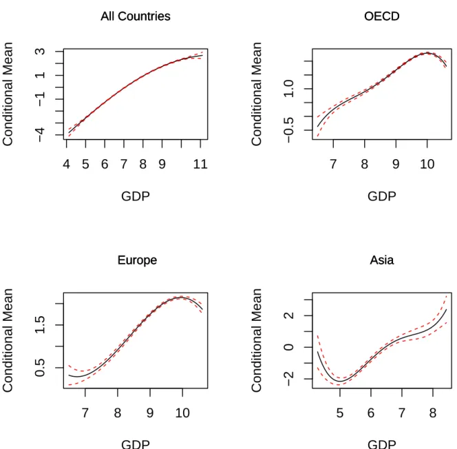
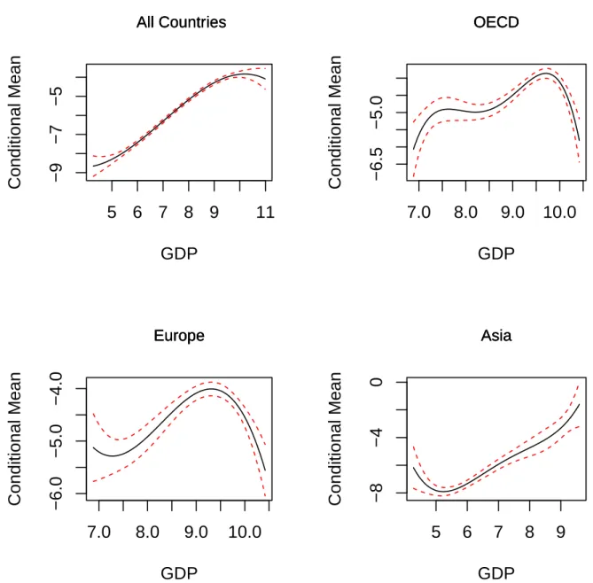
We supplement the above analysis with non-parametric graphical robustness checks, using the spline-based method from Ma, Racine and Yang (2011) and Racine and Nie (2011). This method provides a graphical representation of the mean of the emissions series conditional on contemporaneous GPD. The conditional mean is assumed to follow a non-linear and unknown function approximated via best-…t B-splines allowing for heteroskedasticity of unknown form (again assumed to depend on GDP). Further details are in the Appendix. Reported results do not use other controls. Re‡ecting available technological known-how in this literature, such estimations do not account for the panel structure of the data, nor for its time series proper-ties, and impose stationarity.15 For this reason, we do not interpret resulting curves from an inferential perspective. Instead, we view them as summary representations of our data. Severe inconsistencies between these curves and our parametric results are nevertheless worth checking
1 5To some extent, aside from the shape restriction, the non-parametric assumptions are not necessarily weaker
for. In particular, we look for asymmetries in the estimated function in addition to turning points, since - although not required for an EKC - our quadratic parametric equations imposes symmetry.
3
Estimation Uncertainty for Tipping Points
Assuming the considered estimators are consistent and asymptotically normal, the Delta-method provides Wald-type con…dence intervals using regular asymptotic theory. To present our set estimators in their simplest form with reference to the problem at hand16, let us reparametrize equation (2.1) into a panel regression of EMit on GP Dit [with coe¢ cient 1], GDPit2=2 [with coe¢ cient 2] and all remaining controls, so that the tipping point becomes = exp( 1= 2), with estimators ^ = exp(^1=^2). Let
^12= ^v1 v^12 ^ v12 v^2
refer to the subset of the variance/covariance matrix of the estimates that corresponds to ^1 and ^2. The Delta method leads to the usual Wald-type 1 level con…dence interval:
DCS ( ; ) =h^ z =2^1=2i; ^ = ^G0^12G; ^^ G = ^ 1=^2; ^1=^ 2 2
0
(3.5) where z =2 refers to the two-tailed -level standard normal cut-o¤ point. The solution is pre-sented in Appendix B. The Delta-method for (1 ) level thus requires inverting the t-statistic associated with HD( 0) : 0 = 0
tD( 0) = ^ 0 = h
^1=2i ;
where inverting a test with respect to a parameter means collecting all values (here 0) not rejected by this test at the level. This de…nition relies on the usual duality between a t-test and a standard con…dence interval.
In contrast, the Fieller method inverts an alternative t-statistic tF(d0) = (^1 d0^2)=[(^v1+ d20v^2 2d0v^12)1=2]
associated with HF(d0) : 1 d0 2= 0, where d0 = log( 0). This requires solving for the set of d0 values that are not rejected at level using tF(d0) and a standard normal two-tailed cut-o¤ z =2. In other words, we need to collect the d0 values such that jtF(d0)j z =2 or alternatively such that (^1 d0^2)2 z2=2(^v1+ d20^v2 2d0v^12), leading to a second degree inequality in d0. The resulting set denoted FCS (d; ) [see (B.4) in Appendix B] will have (1 ) level whether 2 is zero or not. The solution for the underlying inequality is provided in Appendix B. FCS (d; ) is either a bounded interval, an unbounded interval, or the entire real line ] 1; +1[, where
1 6
the unbounded solutions occurs when the denominator is close to zero. Because FCS (d; ) is obtained by projection methods, taking the exponential of its limits provides the desired con…dence set for .
In parallel, the considered non-parametric method [see Racine and Nie (2011) for details] yields estimates and con…dence bands for the point at which the derivative of the estimated function is closest to zero. We take the latter as our tipping point estimate in cases where an inverted-U shape is non-parametrically con…rmed. This analysis, as argued above, aims to check for severe inconsistencies between our parametric and non-parametric results. In particular we aim to assess robustness of the tipping point estimates to the symmetry hypothesis underlying our quadratic equations.
3.1 Results
Tables 1-2 report estimates for the emission equation coe¢ cients. For presentation clarity, we report the estimates of the parameters of interest j, j = 1; :::5; complete results are available upon request. Since sign restrictions have not been empirically imposed, interpretation of the tipping point with respect to an inverted U-shaped curve make sense when 1 > 0 and 2 < 0. So cases where the estimated 1 and 2 are signi…cant at the 5% level and both are correctly signed are reported in bold characters. Except for a few illustrative cases, our analysis will focus on these cases, mainly for concreteness. In our discussion from there on, statistical signi…cance implies a 5% level. Tipping point estimates are reported in Tables 3-5.
From Tables 1 and 2, we see that a statistically insigni…cant 2 occurs quite often with both emission series. As argued above, despite no clear consensus, a linear EKC is not necessarily at odds with the current literature. Problems with the Delta method for inference on the tipping point would occur if the true 2 is zero, so a signi…cant 2 does not necessarily guarantee identi…cation. We nevertheless view these results as a motivation in support of the Fieller method whose accuracy does not depend on a non-zero 2. Indeed, unbounded con…dence sets are quite prevalent in Tables 3-5, which con…rm that the tipping point is indeed hard to pin down from available data.
Another point worth emphasizing concerns the heterogeneity of results across regions, with all estimation methods and both emissions data. Our disaggregate estimation is thus more meaningful than the full sample case, which we nevertheless report for completion and possibly for comparison with available literature. Our discussion will thus focus on our regional estimates. A few methodological comments emerge from Tables 3-5 that are worth pointing out, given that to the best of our knowledge, identi…cation problems have not been formally discussed in this literature.
1. Conforming with econometric theory, the Fieller and Delta method provide comparable con…dence bands when the Fieller set is bounded and tight [as in e.g. Table 5 for the OECD], suggesting strong identi…cation. In this case, the Fieller sets are wider to some extent yet they convey conformable economic content.
2. When the Fieller sets are unbounded and/or very wide suggesting weak identi…cation (which occurs most prominently but not exclusively when a linear curve cannot be refuted)
then the Delta and Fieller sets can be very di¤erent and imply very di¤erent economic conclusions. For example, they may provide con‡icting evidence regarding the statisti-cal signi…cance of the tipping point which may be tested [given the duality between the con…dence intervals and Wald tests] by checking whether the reported sets cover zero. Ex-amples of such a con‡ict include the case of Asia with Carbon and the 2SLS method, the case of Central America with Carbon and the LSDV method, and the noteworthy case of the OECD with Sulphur and the LSDV method. In the latter case, the Delta con…dence set is tight and covers zero, whereas the Fieller set although very wide excludes zero. Since 1 and 2 are signi…cant at the 5% level and both are correctly signed in this case, results with the Delta method with regards to the tipping point seem puzzling. In contrast, the Fieller method reveals that estimation uncertainty is severe in this case, which undermines the usefulness of the estimated curve with this method and the Sulphur series.
3. Other "pathological" results include cases for which the Delta-method based sets are very tight [examples occur more prominently in table 4] while their Fieller counterparts are unbounded. Econometric theory suggests that such cases illustrate [again, on recalling the duality between con…dence intervals and Wald tests] severe spurious rejections with standard methods that do not cater for weak identi…cation. In other words, econometric theory suggests that identi…cation concerns conveyed via unbounded Fieller sets implies that the Delta-method interval may be tightly centered on "wrong" values.17
Tables 3-5 suggest further substantive conclusions. When referring to the "existence" of the EKC, a broad de…nition that prevails in the literature entails the following: emission levels initially rise with per capita income but then eventually fall as per capita income exceeds some threshold level. Viewed collectively, our results suggest that conforming with this de…nition, the estimated 1 and 2 are signi…cant at the 5% level and both are correctly signed mainly in the OECD region. This conclusion while not at odds with the literature needs to be quali…ed, when interpreting results on the tipping point estimates. Except with the long-run dynamic …xed e¤ects method applied to the OECD region, estimates of the tipping points are either extremely imprecise (practically uninformative), or suggest economically implausible values. Although quite wide, the Delta method does not convey how seriously uninformative these sets truly are. Consider for example the case of Carbon with the 2SLS estimate form Table 2, in the OECD region. In this case, both estimation methods support an inverted-U curve, yet the con…dence intervals suggest a lower bound of at least 46:687, which is disconcerting given our measure of per capita income in thousands of constant 2000 USD. It may be argued that from a purely statistical perspective, both set estimates are not too wide, indicating that can be pinned down with enough precision. From an economic perspective, these estimates are much too high to reconcile with meaningful useful theory or useful policy. It is interesting to note that using Sulphur for this same region and this same method rejects the EKC form, which is re‡ected via highly imprecise estimates of the tipping point. Although wide, the Delta method based bands understate the severity of estimation uncertainty in this case. With the bias-corrected LSDV
1 7
Indeed, the above cited econometric literature provides many convincing simulation studies documenting this problem with standard Wald-type tests.
method, we …nd support for the curve with both emission series for the OECD countries. Yet the estimate uncertainty regarding the tipping point is much more pronounced than with the 2SLS method, so for all practical purposes, LSDV-based con…dence intervals are non-informative.
On balance, results via our long-run approach in Table 5 for the OECD are informative and consistent with EKC predictions. Con…dence bands suggest, in addition to statistical precision, turning points that are economically reasonable given our measurement scale for GDP. These results may be attributed to various methodological considerations. First, it matters importantly to account for dynamics in estimating the EKC. Second, avoiding methods that are not designed for …xed n is commendable. The bias-corrected LSDV method is in principle applicable, yet the bias-correction assumes strictly exogenous regressors. The pooled long-run inference methods are designed for …xed n and large T . "How large is large" is of course a usual question with annual data. The fact remains that …xed n-and-T panel data methods are unavailable to date, so given the emissions series at hand and the importance of a regional analysis, one may argue that dynamic …xed e¤ects are, among available methods, best suited for our purpose. Perhaps more importantly, in contrast to other cointegration methods, dynamic …xed e¤ects do not require one to take a stand regarding the I(1) properties of regressors. Given available mixed results in this literature, this is worth pointing out. Of course this presumes that the considered long-run relations are stable and that estimations with further lags (to control for potential endogeneity of regressors) provide conformable results. Our results for the OECD region do not seem to refute these assumptions.
It is worth noting that our estimated turning points are generally lower with SO2 than with CO2. This suggests that results with local pollutants may be more relevant from a policy perspective. Since European countries share some common regulations with regards to local pollutants, we revisit our analysis of the OECD countries with focus on Europe. Results reported in Table 6 support our main message: policy-relevant estimates of the tipping point are recovered via a dynamic long-run econometric perspective. From a technical perspective and comparing Table 6 to the OECD results from Table 5, note that a decreased sample size costs statistical precision with the CO2 data. With this series, we …nd sizable di¤erences in con…dence bands when including and excluding the long run control variables. Interestingly, the SO2 case is more stable, which supports our reliance on local pollutants in analyzing this sub-sample. This also leads us to revisit the Central America results, since a local pollutant argument may be relevant for this sub-sample with SO2 data. Indeed, Table 5 suggests evidence in favour of an EKC with reasonable tipping points in this case as well.
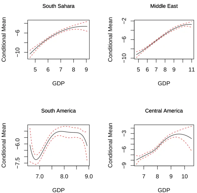
Finally, our non-parametric analysis reported in Figures 1-2 may help further understand the above results. Indeed, for most non-OECD countries, observed best …t curves deviate arbitrarily and dramatically from an expected EKC. Even if a formal statistical test is not intended, such inconsistencies [between the postulated parametric quadratic form and its non-parametric best-…t counterpart] may justify - at least in part - the severe uncertainties we …nd via parametric estimates of the tipping point. In contrast, non-parametric curves for the OECD countries are globally in line with our parametric results; the same observation holds for Central America with SO2. Some asymmetry in cases where an EKC was found is suggested yet appears minor. Some of the observed clustering and bunching-up may also be attributed to the fact that dynamic
and country e¤ects are not accounted for. For reference [and because reported …gures are in a log-scale] companion non-parametric tipping point set estimates conformable with Tables 1-6 are reported in Table 7. Although non-parametric con…dence bands in Table 7 are tighter than their parametric counterparts from Tables 5 and 6, both convey fairly comparable substantive information. This is worth noting, because (in contrast with our parametric methods) non-parametric estimations do not account for the panel, endogeneity and time series structure of the data, and require stationarity.
4
Conclusion
Despite some overemphasis on methodology in recent works, important advances in economet-rics have made empirical work on the EKC seem more credible than it was in the early nineties. Our contributions to estimating the EKC focus on the precision of the tipping point estimate, under various assumptions regarding endogeneity and persistence, and functional form. Taken collectively, our results suggest that except from a local-pollutant long-run or non-parametric perspective, con…dence sets around the tipping point are su¢ ciently wide that the policy rele-vance of the EKC is greatly undermined even in the OECD. From a constructive perspective, we view these results as a motivation for further work aiming to improve identi…cation of the curve, and for …nite sample motivated panel data methods.
The fact that a long-run approach holds promise - although noteworthy - should not be viewed as evidence in favour of a cointegration approach to the EKC. In the same vein, our non-parametric estimations - although informative - are not intended to disqualify parametric estimations (recall that as considered, the former are not necessarily less restrictive than the latter). Rather, our main conclusion is that regardless of the statistical assumptions one is comfortable maintaining in this context, interpreting the shape of the curve should not be the whole story. We should and do ask whether data supports a plausible tipping point. To do so, statistical methods that account for a weakly identi…ed tipping point should be preferred, because of the nature of the problem under study. Indeed, if the question taken to the data is whether a non-linear e¤ect is present, then methods that impose the linear case away - which causes weak identi…cation - cannot be adequate.
Table 1 - Carbon Emissions Equation
All OECD Asia SS-Africa M. East S. America C. America
2SLS GDP 0.550 1.262 0.427 0.336 0.883 0.497 -0.007 (0.00) (0.00) (0.00) (0.00) (0.00) (0.00) (0.95) GDP2 0.002 -0.113 0.065 0.128 0.011 -0.037 0.362 (0.633) (0.00) (0.00) (0.00) (0.47) (0.52) (0.00) CIE 0.349 0.352 0.434 1.152 0.085 0.093 -1.134 (0.00) (0.00) (0.00) (0.00) (0.24) (0.15) (0.00) EF F 0.755 0.698 1.084 0.432 0.533 0.795 2.587 (0.00) (0.00) (0.00) (0.00) (0.00) (0.00) (0.00) IN D 0.123 0.237 0.337 0.244 -0.035 0.176 0.809 (0.00) (0.00) (0.00) (0.00) (0.70) (0.01) (0.00) DLSDV GDP 0.208 0.347 0.114 0.251 0.170 0.049 0.313 (0.00) (0.00) (0.00) (0.02) (0.00) (0.58) (0.00) GDP2 0.002 -0.039 0.014 0.044 0.017 0.033 0.092 (0.69) (0.00) (0.01) (0.23) (0.23) (0.36) (0.01) CIE 0.182 0.083 0.090 0.597 0.197 0.050 0.136 (0.00) (0.00) (0.00) (0.00) (0.00) (0.08) (0.00) EF F 0.295 0.148 0.320 0.304 0.019 0.240 0.365 (0.00) (0.00) (0.00) (0.00) (0.95) (0.00) (0.00) IN D 0.046 -0.005 0.078 0.033 -0.040 0.048 0.050 (0.02) (0.82) (0.04) (0.56) (0.45) (0.34) (0.28) DFE (A) GDP 0.934 2.837 1.097 1.020 0.758 1.033 1.496 (0.00) (0.00) (0.00) (0.011) (0.00) (0.04) (0.00) GDP2 -0.115 -0.530 -0.045 0.331 -0.044 -0.086 -0.139 (0.00) (0.00) (0.59) (0.13) (0.44) (0.69) (0.41) DFE (B) GDP 0.619 1.645 0.494 0.379 0.758 0.532 0.356 (0.00) (0.00) (0.00) (0.014) (0.00) (0.18) (0.18) GDP2 -0.007 -0.191 0.047 0.070 -0.048 0.049 0.199 (0.66) (0.00) (0.14) (0.38) (0.38) (0.77) (0.04) CIE 0.331 0.30 0.270 0.885 0.307 0.121 0.165 (0.00) (0.03) (0.02) (0.00) (0.00) (0.36) (0.09) EF F 0.768 0.913 1.047 0.457 2.847 0.741 0.830 (0.00) (0.00) (0.00) (0.00) (0.08) (0.00) (0.00) IN D 0.154 0.403 0.594 0.049 -0.307 0.034 0.028 (0.02) (0.02) (0.00) (0.66) (0.16) (0.86) (0.79) 2SLS: Baltagi and Li (1992); equation: (2.1), with time dummies;GDP,GDP2, CIE instrumented using …rst lags. DLSDV: Kiviet (1995); equation: (2.3) with time dummies and j= 0,j = 1; :::5. DFE: Pesaran, Shin and Smith (1999); equations (2.3) with j= 0,j = 3; :::5(Case A) and relaxing the latter constraints (case B). In bold: 1 and 2 signi…cant at 5% with 1> 0and 2< 0.
Table 2 - Sulphur Emissions Equation
All OECD Asia SS-Africa M. East S. America C. America
2SLS GDP 0.819 1.062 0.784 -0.723 2.184 0.252 -3.046 (0.00) (0.01) (0.00) (0.03) (0.00) (0.18) (0.00) GDP2 -0.054 -0.327 0.016 0.038 0.286 0.305 1.537 (0.06) (0.14) (0.66) (0.01) (0.00) (0.46) (0.00) CIE -0.099 1.829 0.184 -1.056 -1.902 -0.213 0.766 (0.43) (0.00) (0.13) (0.78) (0.00) (0.07) (0.32) EF F 0.449 -0.846 0.719 1.772 1.184 0.850 2.027 (0.04) (0.13) (0.00) (0.00) (0.50) (0.00) (0.00) IN D 0.052 0.190 0.668 3.556 -1.006 0.583 -0.469 (0.73) (0.65) (0.01) (0.00) (0.03) (0.011) (0.00) DLSDV GDP 0.231 0.621 0.244 -0.096 0.270 -0.096 -1.998 (0.00) (0.03) (0.011) (0.66) (0.37) (0.62) (0.02) GDP2 -0.021 -0.127 0.007 -0.048 -0.044 0.058 0.980 (0.14) (0.03) (0.72) (0.56) (0.44) (0.54) (0.00) CIE -0.041 0.180 -0.002 0.174 -0.131 0.008 0.063 (0.37) (0.05) (0.96) (0.08) (0.21) (0.89) (0.74) EF F 0.053 -0.187 0.274 0.374 -0.374 0.177 0.604 (0.60) (0.33) (0.02) (0.14) (0.83) (0.28) (0.28) IN D 0.060 -0.101 -0.041 0.117 0.035 0.070 0.209 (0.41) (0.60) (0.77) (0.42) (0.89) (0.58) (0.51) DFE (A) GDP 0.825 3.115 0.513 1.194 0.934 -0.423 -2.196 (0.00) (0.00) (0.03) (0.00) (0.03) (0.68) (0.03) GDP2 -0.155 -0.666 -0.118 -0.313 -0.172 0.574 1.209 (0.00) (0.00) (0.21) (0.04) (0.06) (0.26) (0.01) DFE (B) GDP 0.564 3.092 0.169 -0.065 1.256 -1.199 -2.073 (0.00) (0.00) (0.41) (0.88) (0.02) (0.21) (0.06) GDP2 -0.081 -0.627 -0.041 -0.088 -0.170 0.850 1.037 (0.05) (0.00) (0.59) (0.53) (0.06) (0.05) (0.02) CIE -0.065 1.058 0.114 -0.054 -0.620 0.170 0.370 (0.57) (0.00) (0.57) (0.80) (0.00) (0.59) (0.39) EF F 0.896 -0.680 1.095 1.861 -4.030 1.973 0.456 (0.00) (0.18) (0.01) (0.00) (0.20) (0.04) (0.63) IN D 0.193 -0.301 0.182 -0.011 0.244 -0.327 0.785 (0.32) (0.52) (0.073) (0.97) (0.52) (0.68) (0.14) 2SLS: Baltagi and Li (1992); equation: (2.1), with time dummies;GDP,GDP2, CIE instrumented using …rst lags. DLSDV: Kiviet (1995); equation: (2.3) with time dummies and j= 0,j = 1; :::5. DFE: Pesaran, Shin and Smith (1999); equations (2.3) with j= 0,j = 3; :::5(Case A) and relaxing the latter constraints (case B). In bold: 1 and 2 signi…cant at 5% with 1> 0and 2< 0.
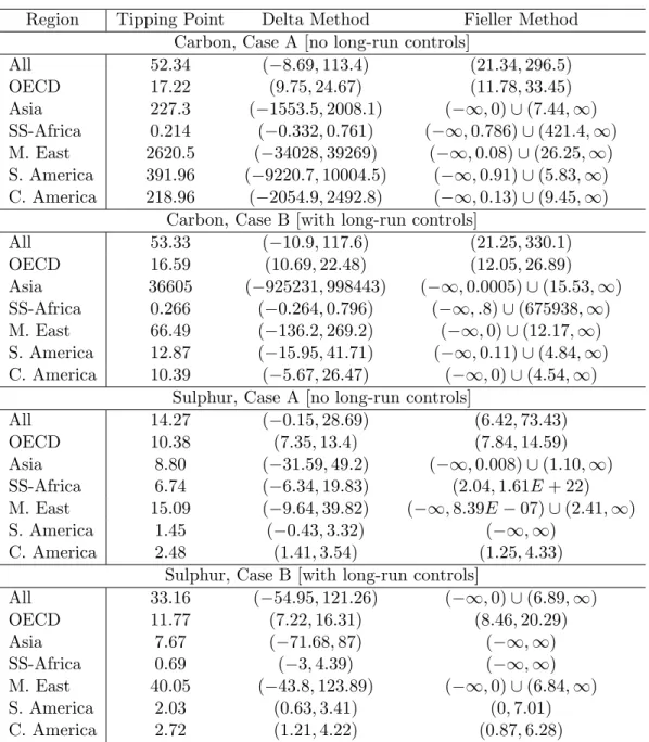
Table 3: Set estimates for the tipping point using panel 2SLS
Region Tipping Point Delta Method Fieller Method
Carbon Dioxide
All 2:6E + 21 ( 2:2E + 23; 2:2E + 23) ( 1; 0) [ (1:04E + 08; 1)
OECD 95:76 (46:687; 144:835) (61:35; 176:06)
Asia :039 ( 0:011; 0:091) (0:006; 0:107)
SS-Africa :269 (0:054; 0:485) (0:061; 0:477)
M. East 5:52E 18 ( 6E 16; 6E 16) ( 1; 0:0001) [ (8E + 10; 1) S. America 797:92 ( 12965:8; 14561:6) ( 1; 0:211) [ (11:17; 1)
C. America 1:009 (0:729; 1:29) (0:708; 1:279)
Sulphur
All 1854:92 ( 10137:13846:8) ( 1; 0) [ (73:40; 1)
OECD 25:86 ( 27:92; 79:64) ( 1; 0:07) [ (9:49; 1)
Asia 8:02E + 10 (0; 8:073E + 12) ( 1; 0:0004) [ (78:90; 1) SS-Africa 8:02E 05 ( 0:005; 0:0054) ( 1; 0:44) [ (3:16; 1)
M. East 45:22 ( 11:62; 102:06) (19:82; 824:63)
S. America 0:66 ( 0:32; 1:647) ( 1; 1:47) [ (1:21E + 08; 1)
C. America 2:69 (2:489; 2:899) (2:49; 2:91)
Estimating equation: (2.1), with time dummies. Method: error component 2SLS from Baltagi and Li (1992). GDP, GDP2 and CO2 Intensity are instrumented using the …rst lag of each. All con…dence sets are at the 5% level.
Table 4. Set estimates for the tipping point using dynamic bias-corrected LSDV
Region Tipping Point Delta Method Fieller Method
Carbon Dioxide
All 1:45E + 21 ( 127:35; 2:57E + 23) ( 1; 0) [ (46852; 1)
OECD 56:924 (2:613; 138:23) (19:47; 814:4) Asia 0:036 ( 7:44; 0:184) ( 1; 0:336) [ (9E + 9; 1) SS-Africa 0:059 ( 9:93; 0:481) ( 1; 1:02) [ (29:66; 1) M. East 0:008 ( 20:61; 0:146) ( 1; 1:07) [ (149:1; 1) S. America 0:765 ( 4:722; 4:178) ( 1; 1) C. America 0:199 ( 3:80; 0:637) (0:00004; 0:724) Sulphur All 223:19 ( 1100:2; 1546:6) ( 1; 6:69E 05) [ (9:34; 1) OECD 11:44 ( 4:42; 27:29) (1:81; 10390:11)
Asia 1:12E 08 ( 1:1E 6; 1:13E 06) (0:14; 11:26)
SS-Africa 0:36 ( 1:98; 2:71) ( 1; 1)
M. East 21:68 ( 52:1; 95:49) ( 1; 1)
S. America 2:29 ( 2:23; 6:81) ( 1; 1)
C. America 2:77 (1:42; 4:11) (1:36; 4:40)
Estimating equation: (2.3) with time dummies and j= 0,j = 1; :::5. Relaxing the latter constraints increases uncertainty with both emission series. Method: bias-corrected LSDV with bootstrap standard errors from Kiviet (1995) and Bruno (2005). All con…dence sets are at the 5% level.
Table 5. Set estimates for the tipping point using long-run dynamic …xed e¤ects Region Tipping Point Delta Method Fieller Method
Carbon, Case A [no long-run controls]
All 52:34 ( 8:69; 113:4) (21:34; 296:5) OECD 17:22 (9:75; 24:67) (11:78; 33:45) Asia 227:3 ( 1553:5; 2008:1) ( 1; 0) [ (7:44; 1) SS-Africa 0:214 ( 0:332; 0:761) ( 1; 0:786) [ (421:4; 1) M. East 2620:5 ( 34028; 39269) ( 1; 0:08) [ (26:25; 1) S. America 391:96 ( 9220:7; 10004:5) ( 1; 0:91) [ (5:83; 1) C. America 218:96 ( 2054:9; 2492:8) ( 1; 0:13) [ (9:45; 1)
Carbon, Case B [with long-run controls]
All 53:33 ( 10:9; 117:6) (21:25; 330:1) OECD 16:59 (10:69; 22:48) (12:05; 26:89) Asia 36605 ( 925231; 998443) ( 1; 0:0005) [ (15:53; 1) SS-Africa 0:266 ( 0:264; 0:796) ( 1; :8) [ (675938; 1) M. East 66:49 ( 136:2; 269:2) ( 1; 0) [ (12:17; 1) S. America 12:87 ( 15:95; 41:71) ( 1; 0:11) [ (4:84; 1) C. America 10:39 ( 5:67; 26:47) ( 1; 0) [ (4:54; 1)
Sulphur, Case A [no long-run controls]
All 14:27 ( 0:15; 28:69) (6:42; 73:43) OECD 10:38 (7:35; 13:4) (7:84; 14:59) Asia 8:80 ( 31:59; 49:2) ( 1; 0:008) [ (1:10; 1) SS-Africa 6:74 ( 6:34; 19:83) (2:04; 1:61E + 22) M. East 15:09 ( 9:64; 39:82) ( 1; 8:39E 07) [ (2:41; 1) S. America 1:45 ( 0:43; 3:32) ( 1; 1) C. America 2:48 (1:41; 3:54) (1:25; 4:33)
Sulphur, Case B [with long-run controls]
All 33:16 ( 54:95; 121:26) ( 1; 0) [ (6:89; 1) OECD 11:77 (7:22; 16:31) (8:46; 20:29) Asia 7:67 ( 71:68; 87) ( 1; 1) SS-Africa 0:69 ( 3; 4:39) ( 1; 1) M. East 40:05 ( 43:8; 123:89) ( 1; 0) [ (6:84; 1) S. America 2:03 (0:63; 3:41) (0; 7:01) C. America 2:72 (1:21; 4:22) (0:87; 6:28)
Estimating equation: (2.3) with j= 0,j = 3; :::5(Case A) and relaxing the latter constraints (case B). Method: dynamic …xed e¤ects applied to the error correction form (2.4), from Pesaran, Shin and Smith (1999). All con…dence sets are at the 5% level.
Table 6. Results focusing on Europe
CO2 Tipping Point Delta Method Fieller Method
Panel 2SLS 106:38 (13:42; 199:35) (53:25; 355:08)
Dynamic Bias Corrected LSDV 83:69 ( 14:77; 182:15) (32:49; 445:03) Dynamic Fixed E¤ects - with long run controlls 50:81 ( 0:12; 101:74) (25:65; 436:67) Dynamic Fixed E¤ects - no long run controlls 13:67 (8:31; 19:04) (9:28; 26:38)
SO2 Tipping Point Delta Method Fieller Method
Panel 2SLS 7:64 (5:29; 9:98) (5:81; 12:01)
LSDV 21:52 ( 2:11; 69:16) (3:38; 11703:3)
Dynamic Fixed E¤ects - with long run controls 14:43 (5:11; 23:74) (8:81; 55:62) Dynamic Fixed E¤ects - no long run controls 12:5 (6:08; 18:91) (7:84; 29:29)
Refer to Tables 1-5 for the de…nition of estimation methods. European countries are selected out of the OECD list reported in the Appendix for each emission series.
Table 7. Non parametric tipping point estimates, selected sub-samples CO2 Tipping Point Estimate Estimated Con…dence Bands
OECD 17:61 (15:73; 19:42)
Europe 15:60 (14:61; 16:50)
SO2 Tipping Point Estimate Estimated Con…dence Bands
OECD 10:83 (9:07; 11:71)
Europe 14:77 (12:38; 15:91)
Central America 2:10 (0:63; 3:35)
Refer to the Appendix for the description of the estimation method. European countries are selected out of the OECD list reported in the Appendix for each emission series.
Appendix
A
List of countries
Countries used for the CO2 equation
OECD.18 (27 countries). Albania, Austria, Belgium, Canada, Denmark, Finland, France, Germany, Greece, Hong Kong, Hungary, Iceland, Ireland, Italy, Japan, Malta, Netherlands, New Zealand, Norway, Portugal, South Korea, Spain, Sweden, Switzerland, Turkey, United Kingdom, United States
Asia. (17 countries) Bangladesh, China, India, Indonesia, Kazakhstan, Kyrgyzstan, Malaysia, Mongolia, Pakistan, The Philippines, Singapore, Sri Lanka, Tajikistan, Thailand, Turkmenistan, Uzbekistan, Vietnam
Sub-Saharan Africa. (16 countries) Angola, Benin, Botswana, Cameroon, Congo, Cote d’Ivoire, Gabon, Ghana, Kenya, Namibia, Nigeria, Senegal, South Africa, Togo, Zambia, Zim-babwe
The Middle East & North Africa. (16 countries) Algeria, Bahrain, Egypt, Eritrea, Iran, Jordan, Kuwait, Lebanon, Morocco, Oman, Saudi Arabia, Sudan, Syria, Tunisia, United Arab Emirates, Yemen
South America. (11 countries) Argentina, Bolivia, Brazil, Chile, Colombia, Ecuador, Guatemala, Paraguay, Peru, Uruguay, Venezuela.
Central America & The Caribbean. (10 countries). Costa Rica, Dominican Re-public, El Salvador, Haiti, Honduras, Jamaica, Mexico, Nicaragua, Panama, Trinidad & To-bago.
Other. (17 countries) Armenia, Azerbaijan, Belarus, Bulgaria, Croatia, Czech Republic, Georgia, Latvia, Lithuania, Macedonia, Moldova, Poland, Romania, Russia, Slovakia, Slovenia, Ukraine.
Countries used for the SO2 equation
OECD. (27 countries). Albania, Austria, Belgium, Canada, Denmark, Finland, France, Germany, Greece, Hong Kong, Hungary, Iceland, Ireland, Italy, Japan, Malta, Netherlands, New Zealand, Norway, Portugal, South Korea, Spain, Sweden, Switzerland, Turkey, United Kingdom, United States.
Asia. (12 countries). Bangladesh, China, India, Indonesia, Malaysia, Mongolia, Pakistan, Philippines, Singapore, Sri Lanka, Thailand, Vietnam.
Sub-Saharan Africa. (11 countries). Botswana, Cameroon, Cote d’Ivoire, Gabon, Ghana, Kenya, Senegal, South Africa, Togo, Zambia, Zimbabwe.
1 8
The list of OECD countries includes countries that have been in the OECD for the majority of the time frame of this study, with the exceptions of Albania and South Korea. The latter two are included because, in our judgement, are anomalies with respect to their geographic peers and Albania is included because this group corresponded closest to its characteristics.
The Middle East & North Africa. (13 countries) Algeria, Bahrain, Egypt, Iran, Jor-dan, Kuwait, Morocco, Oman, Saudi Arabia, SuJor-dan, Syria, Tunisia, United Arab Emirates. South America. (10 countries). Argentina, Bolivia, Brazil, Chile, Colombia, Guatemala, Paraguay, Peru, Uruguay, Venezuela.
Central America & The Caribbean. (7 countries). Costa Rica, Dominican Republic, El Salvador, Honduras, Mexico, Panama, Trinidad & Tobago.
Other. (2 countries). Bulgaria, Romania.
B
The Fieller method
Consider the general model (Y; fP : 2 g), Rp, p 1, where Y is the sample space and P is a probability distribution over Y indexed by = ( 1; 2; :::; p)0. Our object of interest are functions of of the form h ( ) = exp(L0 =K0 ) where L and K are nonstochastic p 1 vectors. Given a sample of size T , assume a consistent and asymptotically normal estimator of is available ^ = (^1; ^2; :::; ^p)0 asy N( ; ) where is estimated consistently by b . The discontinuity set f 2 : K0 = 0g is clearly non-empty. In this context, the Delta method exploits the following regular asymptotic result:
h(^)asyN 0 @h ( ) ;@h ^ @ 0 ^ @h0 ^ @ 1 A : (B.1)
For the same problem, Fieller’s method inverts a Wald-type test associated with the hypothesis L0 d0K0 = 0 for a collection of …xed d0 values. For the ratio case presented in section 3, Fieller’s method involves assembling all d0 values such that 1 d0 2= 0 is not rejected at the % using the t-statistic ^1 d0^2 = d20^v2 2d0^v12+ ^v1 1=2 which is asymptotically standard normal under the null hypothesis. This requires the solution to the following inequality in d0
FCS ( ; ) = d0 : ^1 d0^2 2
z2=2 ^v1+ d20^v2 2d0v^12 ; leading to the second-degree-polynomial inequality for d0:
A 20+ 2B 0+ C 0 (B.2)
A = ^22 z2=2v^2; B = ^1^2+ z2=2v^12; C = ^ 2
1 z2=2^v1: (B.3) Except for a set of measure zero, A 6= 0. Similarly, except for a set of measure zero, = B2 AC 6= 0. Real roots d01= B p A ; d02= B +p A
exist if and only if > 0, so
FCS (d; ) = [d01; d02] if A > 0 ] 1; d01] [ [d02; +1[ if A < 0
: (B.4)
Bolduc, Khalaf and Yelou (2010) further show that: (i) if < 0, then A < 0 and FCS (d; ) = R; (ii) FCS (d; ) contains the point estimate ^1=^2 and thus cannot be empty, and (iii) asymptot-ically, Fieller’s solution and the Delta method give similar results when the former leads to an interval, i.e. when the denominator is far from zero. Taking the exponential of the limits of FCS (d; ) provides a con…dence set for exp(d).
C
B-splines
Using the method introduced by Ma, Racine and Yang (2011), we estimate the conditional expectation of emissions via the following relationship:
EMit= f (GDPit) + (GDPit)uit; f (:) and (:) unknown, (C.5a) which provides a graphical representation [with con…dence bands] of the mean of emissions conditional on GDP, disregarding the dynamic properties of the model and its panel structure. This method uses a B-spline function for f (:) , which is a linear combination of B-splines of degree m de…ned as follows
B(x) = N +mX
c=0
bcBc;m(x); x 2 [k0; kN +1]
where bc are denoted "control points", k0; :::; kN +1 are known as a knot sequence [an individual term in this sequence is known as a knot],
Bc;0(x) =
1 kc x < kc+1 0 otherwise which is referred to as the ‘intercept’, and
Bc;j+1(x) = ac;j+1(x)Bc;j(x) + [1 ac+1;j+1(x)]Bc+1;j(x); ac;j+1(x) = ( x kc kc+j kc kc+j6= kc 0 otherwise ) :
The unknown function f (GDPit) is estimated by least squares as b B(GDPit) = argminB(GDPit;g) n X i=1 T X t=1 [EMit B(GDPit)]2:
Explicitly, this requires the estimation of the control points bc. Underlying best …t parameters are selected by cross-validation; see Racine and Yang (2011) for further details. Further description of this R-package is available at: http://cran.r-project.org/web/packages/crs/crs.pdf.
To obtain tipping point estimates comparable to those in Tables 1-5, and because reported curves in …gures 1-2 are in a log-scale conforming with our estimating equations, we re…t curves in levels and compute the con…dence bands at the point were the derivative of the estimated functions is the closest to zero. These are reported in Table 7 for selected sub-samples.
References
[1] Anderson T. W. and C. Hsiao (1982). Formulation and Estimation of Dynamic Models Using Panel Data. Journal of Econometrics 18, 47-82.
[2] Arellano M. and S. Bond (1991). Some Tests of Speci…cation for Panel Data: Monte Carlo Evidence and an Application to Employment Equations. Review of Economic Studies 58, 277-297.
[3] Azomahou T., Laisney F. and N. Van (2006). Economic development and CO2 emissions: a nonparametric panel approach. Journal of Public Economics 90, 1347-1363.
[4] Beaulieu M.-C., Dufour J.-M. and L. Khalaf (2011). Identi…cation-Robust Estimation and Testing of the Zero-Beta CAPM, revised and resubmitted to: The Review of Economic Studies.
[5] Bernard J.-T., Idoudi N., Khalaf L. and C. Yélou (2007). Finite Sample Inference Methods for Dynamic Energy Demand Models. Journal of Applied Econometrics 22, 1211-1226. [6] Baltagi B. and Q. Li (1992). A Note on the Estimation of Simultaneous Equations with
Error Components. Econometric Theory 8, 113-119.
[7] Blundell R. and S. Bond (1998). Initial Conditions and Moment Restrictions in Dynamic Panel Data Models. Journal of Econometrics 87, 115-143.
[8] Bolduc D., Khalaf L. and C. Yelou (2010). Identi…cation Robust Con…dence Set Methods for Inference on Parameter Ratios with Applications to Discrete Choice Models. Journal of Econometrics 157, 317-327.
[9] Brock W. A. and M. S. Taylor (2005). Economic Growth and the Environment: A Review of Theory and Empirics. In Handbook of Economic Growth, vol. 1B, ed. P. Aghion and S. N. Durlauf. Amsterdam: North-Holland.
[10] Bruno G. S. F (2005). Estimation and Inference in Dynamic Unbalanced Panel-Data Models with a Small Number of Individuals. Stata Journal, StataCorp LP 5, 473-500.
[11] Bun, M. J. G. and J. F. Kiviet (2006). The E¤ ects of Dynamic Feedbacks on LS and MM Estimator Accuracy in Panel Data Models. Journal of Econometrics 132, 409-444.
[12] Bun, M. J. G. and M. A. Carree (2005). Bias-Corrected Estimation in Dynamic Panel Data Models. Journal of Business and Economic Statistics 23, 200-210.
[13] Carson R. T. (2010). Environmental Kuznets Curve: Searching for Empirical Regularity and Theoretical Structure. Review of Environmental Economics and Policy 4, 3-23.
[14] Cavlovic T., Baker K., Berrens R. and K. Gawande (2000). A Meta-Analysis of the Envi-ronmental Kuznets Curve Studies. Agriculture and Resource Economics Review 29, 32-42.
[15] Cole M. A. (2004). Trade, the Pollution Haven Hypothesis and Environmental Kuznets Curve: Examining the Linkages. Ecological Economics 48, 71-81.
[16] Cole M. A., Rayner A. J. and J. M. Bates (1997). The Environmental Kuznets Curve: an Empirical Analysis. Environment and Development Economics 2, 401-416.
[17] Dasgupta S., Laplante B., Wang H. and D. Wheeler (2002). Confronting the Environmental Kuznets Curve. The Journal of Economic Perspectives 16, 147-168.
[18] Dinda S. (2004). Environmental Kuznets Curve Hypothesis: A Survey. Ecological Economics 49, 431-55.
[19] Dinda S. and D. Coondoo (2006). Income and Emission: a Panel-Data Based Cointegration Analysis. Ecological Economics 57, 167-181.
[20] Dufour J.-M. (1997). Some Impossibility Theorems in Econometrics with Applications to Structural and Dynamic Models. Econometrica 65, 1365-1389.
[21] Dufour J.-M. (2003). Identi…cation, Weak Instruments and Statistical Inference in Econo-metrics. Canadian Journal of Economics 36, 767-808.
[22] Fieller E. C. (1940). The Biological Standardization of Insulin. Journal of the Royal Statis-tical Society (Supplement) 7, 1-64.
[23] Fieller E. C. (1954). Some Problems in Interval Estimation. Journal of the Royal Statistical Society B 16, 175-185.
[24] Figueroa E. B. and R. C .Pastén (2009). Country-Speci…c Environmental Kuznets Curves: a Random Coe¢ cient Approach Applied to High-Income Countries. Estudios de Economia 36, 5-32.
[25] Grossman G. and A. Krueger (1995). Economic Growth and the Environment. Quarterly Journal of Economics 110, 353-77.
[26] Harbaugh W. T., Levinson A. and D. M. Wilson (2002). Re-examining the Empirical Evi-dence for an Environmental Kuznets Curve. Review of Economics and Statistics 84, 541-551. [27] Holtz-Eakin D. and T. M. Selden (1995). Stoking the Fires? CO2 Emissions and Economic
Growth. Journal of Public Economics 57, 85-101.
[28] Jalil A. and Mahmud S. F. (2009). Environment Kuznets curve for CO2 emissions: a Cointegration Analysis. Energy Policy 37, 5167-5172.
[29] Judson, R. A., and A. L. Owen (1999), Estimating Dynamic Panel Data Models: A Guide for Macroeconomists. Economics Letters 65, 9-15.
[30] Kalaitzidakis P., Mamuneas T. and T. Stengos (2011). Greenhouse Emissions and Produc-tivity Growth. Working paper, University of Guelph.
[31] Kiviet J. F. (1995). On Bias, Inconsistency and E¢ ciency of Various Estimators in Dy-namic Panel Data Models. Journal of Econometrics 68, 53-78.
[32] Lee C.-C., Chiu Y-B and C.-H. Sun (2010). The Environmental Kuznets Curve Hypothesis for Water Pollution: Do Regions Matter? Energy Policy 38, 12-23.
[33] Levinson A. (2002). The Ups and Downs of the Environmental Kuznets Curve. In: Recent advances in environmental economics, ed. J. List and A. de Zeeuw. Northhampton, MA: Edward Elgar Publishing.
[34] List J. A. and C. A. Gallet (1999). The Environmental Kuznets Curve: Does One Size Fit All ? Ecological Economics 31, 409-423.
[35] List J. A., Millimnet D. and T. Stengos (2003). The Environmental Kuznets Curve: Real Progress or Misspeci…ed Models? The Review of Economics and Statistics 85, 1038-1047. [36] Ma S., Racine J. S. and L. Yang (2011). Additive Regression Splines With Irrelevant
Cat-egorical and Continuous Regressors. Working paper, McMaster University and Michigan State University.
[37] Ordás-Criado C., Stengos T. and S. Valente (2011). Growth and Pollution Convergence: Theory and Evidence. Journal of Environmental Economics and Management 62, 199-214. [38] Panayotou T. (1997). Demystifying the Environmental Kuznets Curve: Turning a Black
Box into a Policy Tool. Environment and Development Economics 2, 465-484.
[39] Perman R. and D. I. Stern (2003). Evidence from Panel Unit Root and Cointegration Tests that the Environmental Kuznets Curve Does Not Exist. Australian Journal of Agricultural and Resource Economics 47, 325-347.
[40] Pesaran M. H. and R. P. Smith (1995). Estimating Long-Run Relationships from Dynamic Heterogeneous Panels. Journal of Econometrics 68, 79-113.
[41] Pesaran M.H., Shin Y. and R. P. Smith (1999). Pooled Mean Group Estimation of Dynamic Heterogeneous Panels. Journal of the American Statistical Association 94, 621 - 634. [42] Richmond A.K. and R. K. Kaufmann (2006). Is There a Turning Point in the Relationship
Between Income and Energy Use and/or Carbon Emissions? Ecological Economics 56, 176-189.
[43] Racine J. S. and Z. Nie (2011). CRS: Categorical Regression Splines. R package version 0.15-11.
[44] Romero-Avila, D. (2008). Questioning the Empirical Basis of the Evironmental Kuznets Curve for CO2: New Evidence from a Panel Stationary Test Robust to Multiple Breaks and Cross/Dependence. Ecological Economics 64, 559-574.